Short-Circuit Conditions and Thermal Behaviour of Different Cable Formations

Abstract

Modern electrical installations widely use cable formations consisting of a few single cables connected in parallel. In this article, the short-circuit problem is analysed with its influence on cable temperature. In the assumed case study of supply lines, five equivalent cases were considered. Calculations of temperature increase during faults were performed using a simplified method and FEM model. This study shows the differences in calculation methods and points to better solutions in cable arrangements due to safety and operating conditions in cases of faults. Additionally, some problems in the simplified method were identified and pointed out in the range of its application.

1. Introduction

Every function in the modern industrial world needs an energy supply. The most important energy source in many fields of industry is electricity. This fact demands analysis of how electrical energy is delivered to the required loads and how the transmission media operate under faults. It has been known for many years that installations may be designed and built as a single cable creating one phase or a bundle consisting of a few single cables connected in parallel. Such data, together with information on the surrounding environment (ground/air) and cable formation, are included in standards [1]. Correctly designed electrical installations have to be verified according to a few conditions, and among these, short-circuit (SC) conditions can be highlighted. How significant an issue this is in relation to electrical cables in buildings, and the possible negative effects, is discussed in [2]. In the scientific literature, cables and their thermal behaviour have been extensively studied for various problems. Nowadays, a finite element method (FEM) is often used to simulate the influence of electromechanical and thermal issues on the performance of cable properties. An application of the FEM in cable analysis is defined in [3]. The FEM is used to simulate how high-voltage cables operate in a large cross-sectional area (CSA), e.g., 1000 mm² or 1600 mm², as shown in [4,5]. Tools such as FEA software are important in engineering calculations and studies, as it is difficult to carry out a real test using the rated voltage (e.g., 400 kV) and simulate transient states in laboratory tests.

Analytical and numerical calculation methods, an online monitoring method, or a thermal circuit model can be used to assess the temperature rise in the cable during transient states [6,7]. Some researchers developed two branch thermal circuit models to control line parameters and realise the function of dynamic thermal rating (DTR) [8,9]. In [10], the authors present results of a three-branch thermal model. As mentioned in [11], the current value describes the maximal load ability, while the limiting factor is the temperature of the conductor or insulation. The thermal parameters of the conductor can be used to determine the current-carrying capacity in the system [12]. For different conditions, different real current capabilities and power losses can be obtained [13]. Some transient models of cable temperature and current carrying capacity prediction are proposed in the literature [14]. It should be underlined that even in the same installation type, the short-circuit parameters can be different because they depend on the supply source [15]. In [16,17], the authors present results of short-circuit (three-phase and one-phase faults, respectively) analyses conducted in laboratory arrangements, where the tested installation was supplied from the synchronous backup generator. The obtained values clearly show that the energy source has a big impact on the short-circuit waveforms and the revealed energy. The thermal processes during transient states caused by short-circuit currents are mostly analysed only in theoretical and simulation calculations using the FEM [18]. Very few scientific publications present results of measurements and simulations/calculations. In [19], the authors present measured results verified with two calculation methods. This research is related only to single short circuits without any other fault. A calculation method of 1 s admissible short-circuit current for overhead transmission lines, considering aperiodic and periodic components, is presented in [20]. New algorithms to evaluate cable ampacity are still being developed [21]. The ampacity calculations and the effect of changing cable arrangements at the circuit ends in power stations are discussed and the impact on cable rating is illustrated with numerical examples in [22]. This approach of studying even the ends of cable lines in power stations shows the significance of cable ampacity and the thermal conditions and, finally, the resistance of the cable. The problem of resistance variations due to cable arrangement and electromagnetic phenomena is studied in [23].

The problem of SC current flows in cables and their effects is a complex issue. First of all, to conduct real-life testing at a laboratory scale there is a need for an adjustable power source with a relatively wide range of forced currents. Moreover, especially in MV or at higher voltage levels, it is important to maintain a voltage value equivalent to normal conditions of cable work (e.g., to verify dielectric power losses in cable insulation). Therefore, it is hard to conduct such tests in a laboratory and for these purposes it is better to use FEM software, which allows very accurate calculations. Experimental validation of an FEM model was performed in [5]. However, the 400 kV cables were supplied only from a DC low-voltage power source, and all the phenomena existing at normal voltage did not occur.

The development of renewable energy sources, especially offshore wind farms, has prompted some researchers to investigate high-temperature superconductor (HTS) cables and their behaviour during transient states. These studies are carried out using numerical and FEM models for different cable constructions and operating conditions. These problems are presented in [24].

The analysis of SCs is a subject of study not only due to the cable current limits, but also due to the SC current source. In the 21st century, power systems utilise distributed generation. The problem of an appropriate SC current value in LV installations is analysed in [17,25]. At the power system scale, the lack of sufficient and required SC power and the idea of introducing virtual inertia are studied in [26].

Any short circuit that is switched off within the required time can be considered as an adiabatic process with no heat exchange with other parts of the cable installation environment. To the best of the authors’ knowledge, there is a real gap in scientific research on short circuits in single conductor cables formed into bundles and compared with equivalent cables with a large CSA. Therefore, this manuscript examines five cable formations in terms of SCs occurring in the installation and the resulting cable heating. Three cases of initial conditions just before the fault were analysed:

(1)

SC current calculated for each formation using cable parameters and a standard power system impedance (for start temperatures of 30 and 70 °C) (case 1);

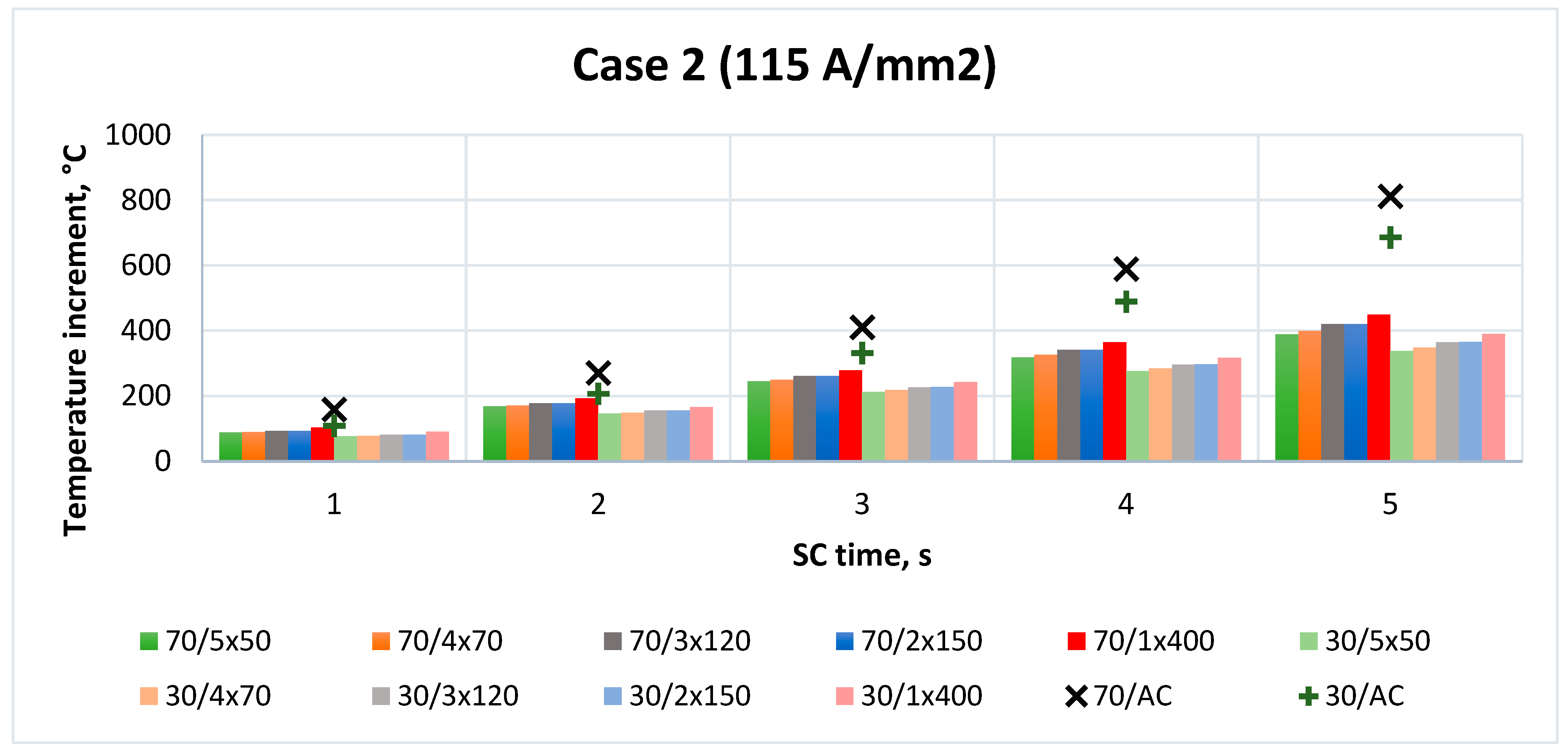
(2)

Short-circuit current corresponding to a constant current density equal to 115 A/mm² (for start temperatures of 30 and 70 °C) (case 2);

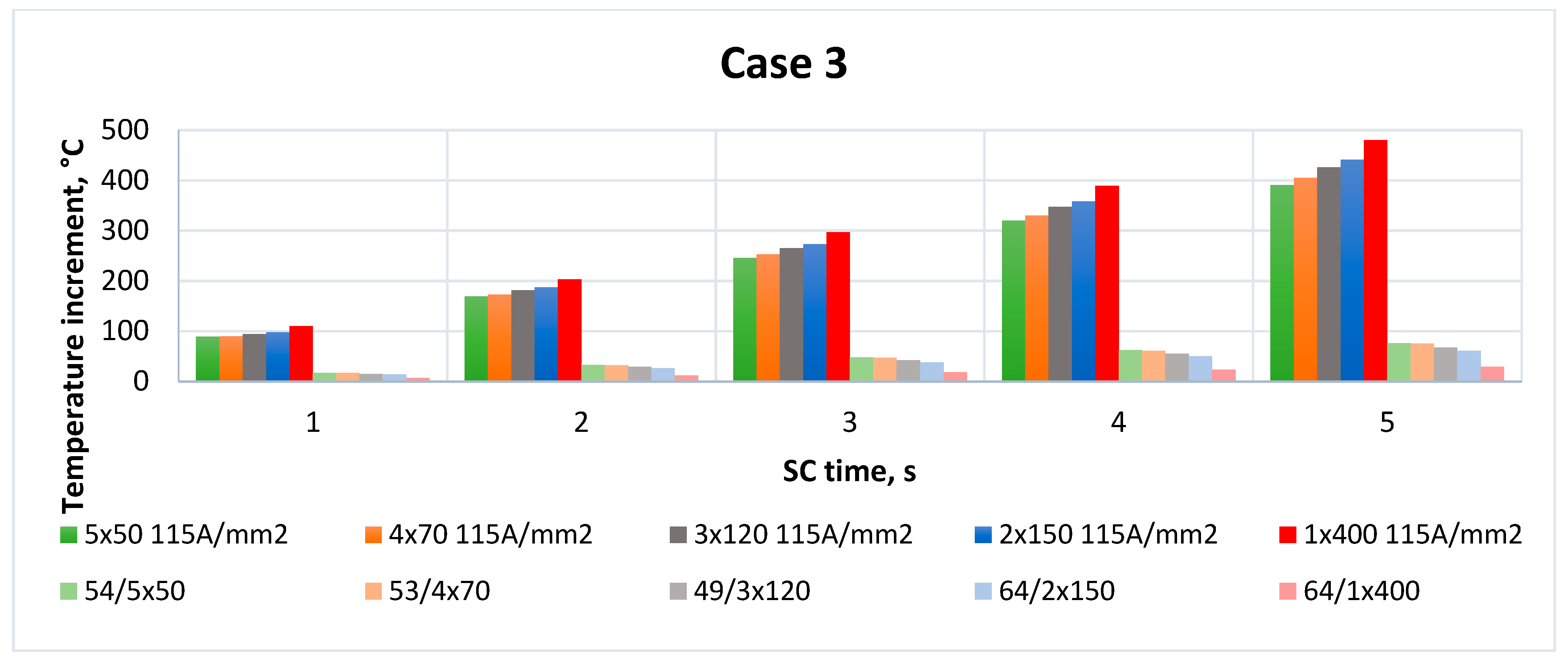
(3)

SC current calculated for each formation for the temperature of the cable after a long-lasting rated load before a fault (case 3).

Such a wide range of analysed cases is prepared to verify the flexibility of simplified methods and FEMs. The results show that some conditions are not suitable to use fast and simplified analytical methods, and to set the real temperature of the cable during a fault, the FEM model has to be prepared and calculations have to be performed.

This manuscript has five sections: the Introduction, then in the Materials and Methods are described the theoretical assumptions and problem formulation. The third section presents results of calculations in both methods, and in the next section the discussion is provided. The last one contains conclusions which briefly summarise the article and point to further research needs.

2. Materials and Methods

2.1. Calculation Methods

To calculate the temperature increment in the conductors, FEM software (femm 4.2) needs to be applied. It is a result of calculations partial difference equations (PDEs) which are formulated in Equation (1):

$$\begin{gathered} k_c{\displaystyle \frac{{\partial }^{2}T}{\partial x^2}}+k_c{\displaystyle \frac{{\partial }^{2}T}{\partial y^2}}=-q_{v,c} \\ {k}_{ins}{\displaystyle \frac{{\partial }^{2}T}{\partial x^2}}+k_{ins}{\displaystyle \frac{{\partial }^{2}T}{\partial y^2}}=0 \\ {k}_s{\displaystyle \frac{{\partial }^{2}T}{\partial x^2}}+k_s{\displaystyle \frac{{\partial }^{2}T}{\partial y^2}}=0 \end{gathered}$$

(1)

where: $T$—temperature value, K; $k_c,k_{ins},k_s$—thermal conductivity of conductor (401 ${\displaystyle \frac{W}{mK}}$), insulation (0.285 ${\displaystyle \frac{W}{mK}}$), outer sheath (0.285 ${\displaystyle \frac{W}{mK}}$), respectively; $x,y$—coordinates of a specific location, m; $q_{v,c}$—heat flux, ${\displaystyle \frac{W}{m^3}}$.

Additionally, due to the fact that this research is conducted in air, the convection phenomenon has to be considered—Equation (2):

$$k{\displaystyle \frac{\partial T}{\partial n}}+\alpha (T-T_0)=0$$

(2)

where: $\alpha$—heat transfer coefficient (10 ${\displaystyle \frac{W}{m^{2}K}}$); $T_0$—ambient cooling fluid temperature (30 °C); $n$—direction normal to the boundary, m.

The heat flux is set based on the SC value and resultant resistance of each conductor. The resistance is recalculated in each step due to the temperature increase according to Equation (3):

$$R_{\left(T\right)}=R_{DC}(1+{\alpha }_T(T-T_{20}\left)\right)$$

(3)

where: $R_{DC}$—resistance for DC current at 20 °C; ${\alpha }_T$—coefficient of thermal expansion (0.0039 ${\displaystyle \frac{1}{K}}$).

For further calculations of the thermal effects of the SC, two cases were considered. In the first one, the same parameters of the power system (resistance 0.001 Ω and inductive reactance 0.001 Ω) for all formations and then resultant parameters specific to the given arrangements are used. In the second one, each formation operates with SC current density equal to 115 A/mm², which is the highest permissible value according to the standard [1]. It should be underlined that this resultant value is clearly a theoretical one and presents how the conductor could operate. In the entire process of an installation design, the condition of minimal CSA must be fulfilled according to the SC parameters in that section of the supply line and the authors are aware of exceeding this condition. In terms of the beginning conductor temperature, the following values are used: 30 °C (which refers to the SC immediately after switching on the supply), 70 °C (which refers to the SC for maximal long-term permissible temperature), and the third one is a result of the temperature for the load current for each formation. The FEM calculations are performed using models prepared according to catalogue data [27] which are presented in Table 3.

The calculations are performed in the FEMM software (femm 4.2) investigating heat flow problems. The boundary conditions are implemented according to the Dirichlet ones (30 °C) and these boundaries are placed at a large distance from the studied objects to eliminate the impact of the edges and examine only relations between cables during the SC.

Due to the short length of the fault durations, the entire heating process is considered as an adiabatic one. This fact allows the use of simplified methods to verify and validate obtained results. The simplified method assumes that the adiabatic process causes no heat emission from the cable. Therefore, using current density, the conductor temperature can be calculated.

One simplified method which allows the performance of fast calculations is using Franz–Wiedemann law for metal conductors (Equation (4)).

$$k\sigma =LT$$

(4)

where: $L$—Lorentz constant, ${\displaystyle \frac{V^2}{K^2}}$; $\sigma$—metal conductivity, $\mathrm{\Omega }\mathrm{m}$; $k$—specific thermal conductivity, ${\displaystyle \frac{W}{mK}}$.

Based on Equation (4) and current density it is possible to set the temperature of the cable according to Equation (5):

$$T_k=\left(273+T_0\right){\mathrm{e}}^{J^2{\displaystyle \frac{L{t}_k}{Ck\rho }}}-273$$

(5)

where: $t_k$—SC flow time, s; $C$—specific heat, ${\displaystyle \frac{\mathrm{J}}{\mathrm{k}\mathrm{g}·°\mathrm{C}}}$; $\rho$—material density, ${\displaystyle \frac{\mathrm{k}\mathrm{g}}{{\mathrm{m}}^3}}$.

The maximal permissible temperature for the SCs is assumed according to standards IEC 60502 [28] and IEC 60724 [29]. For PVC cables greater than 300 mm² it is equal to 140 °C and for other cases 160 °C. The SC maximal duration is 5 s.

2.2. Cable Arrangement Parameters

In this research only low-voltage cables with PVC insulation and an outer sheath are investigated. The parameters of these cables are included in

Table 1. Parameters of single core cables used in the analysis.

CSA, mm2	Current Capacity in Air, A	Current Capacity in Ground, A	Maximal Conductor Resistance, Ω/km	Inductivity, mH/km
50	215	293	0.387	0.294
70	272	363	0.268	0.279
120	389	496	0.153	0.270
150	447	559	0.124	0.266
400	845	962	0.047	0.251

and

Table 2. Calculated parameters of the formations.

Number of Cables and CSA	Derating Factor, -	Calculated Current Capacity, A	Load Current per Cable, A
5 × 50	0.75	807	148.4
4 × 70	0.77	838	185.5
3 × 120	0.82	957	247.3
2 × 150	0.88	787	371
1 × 400	1	845	742

. The construction parameters of used cables are in

Table 3. Construction parameters of cables used in research [27].

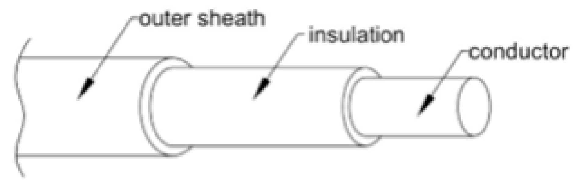
CSA, mm2	Insulation Thickness, mm	Sheath Thickness, mm	Approx. Outer Diameter, mm
50	1.4	1.4	14
70	1.4	1.5	16
120	1.6	1.6	20
150	1.8	1.6	22
400	2.0	2.0	34

and

Table 4. Material parameters used in FEM and simplified calculations.

Parameter	Value
Conductivity of core material, m/(Ωmm2)	55
Relative permeability, -	1
Insulation and sheath thermal conductivity, W/(mK)	0.285
Heat transfer coefficient, W/(m2 K)	10
Ambient cooling temperature of air, °C	30
Thermal conductivity of air, W/(mK)	0.025

and an example of cable construction is depicted in Figure 1.

When cables are formed into bundles, regardless of the shape of the formation, derating factors must be used to verify the current carrying capacity of each cable. The derating factors are available in IEC 60364-5-52 [1]. The cases analysed are summarised in Table 2 along with other additional parameters. The load is assumed to be 742 A per phase, so the load current is divided for each individual cable in the bundle. The total length of the supply line is 200 m.

3. Results

The input values for each case were calculated and are included in

Table 5. Input parameters for all cases.

Formation	Case 1		Case 2		Case 3
	dP30, W	dP70, W	dP30, W	dP70, W	Tin, °C	dPRX, W	dPJd=115, W
5 × 50	2837.7	2553.6	12,481.1	14,382.2	54	2822.4	14,457.1
4 × 70	3727.5	3400.5	17,496.7	20,088.8	53	3771.3	20,313.1
3 × 120	5234.0	4937.7	29,994.3	34,564.9	49	5545.5	35,077.4
2 × 150	6100.1	5835.6	37,492.9	43,146.6	64	6298.0	45,159.2
1 × 400	6351.9	6777.5	99,452.0	114,264.0	64	7348.7	122,139.8

and

Table 6. SC current density.

Formation	Case 1		Case 3/RX
	J30, A/mm2	J70, A/mm2	JRX, A/mm2
5 × 50	55	48	51
4 × 70	53	47	50
3 × 120	48	43	46
2 × 150	46	42	43
1 × 400	29	28	28

. For the third case of the initial temperature before a fault, the values were obtained in a FEM analysis for the steady state at the rated load as it is in Section 2. In Table 5, the indexes are introduced to highlight the following cases: dP₃₀/dP₇₀—power losses for an initial temperature 30/70 °C; dP_Jd=115—power losses for a constant SC current density equal to 115 A/mm² (as in case 2); dP_RX—power losses for constant power system parameters (as in case 1). T_in is the temperature of the conductor at the beginning of the SC for case 3. As one can see in case 1, the increment in the temperature of conductors causes a decrease in power losses in some cases. Only the 1 × 400 bundle results in power loss growth. This is a result of resistance changes and constant power system parameters.

For these prepared input data, the FEM calculations are conducted. The results of these calculations are included in

Table 7. Temperature after SC depending on duration for case 1.

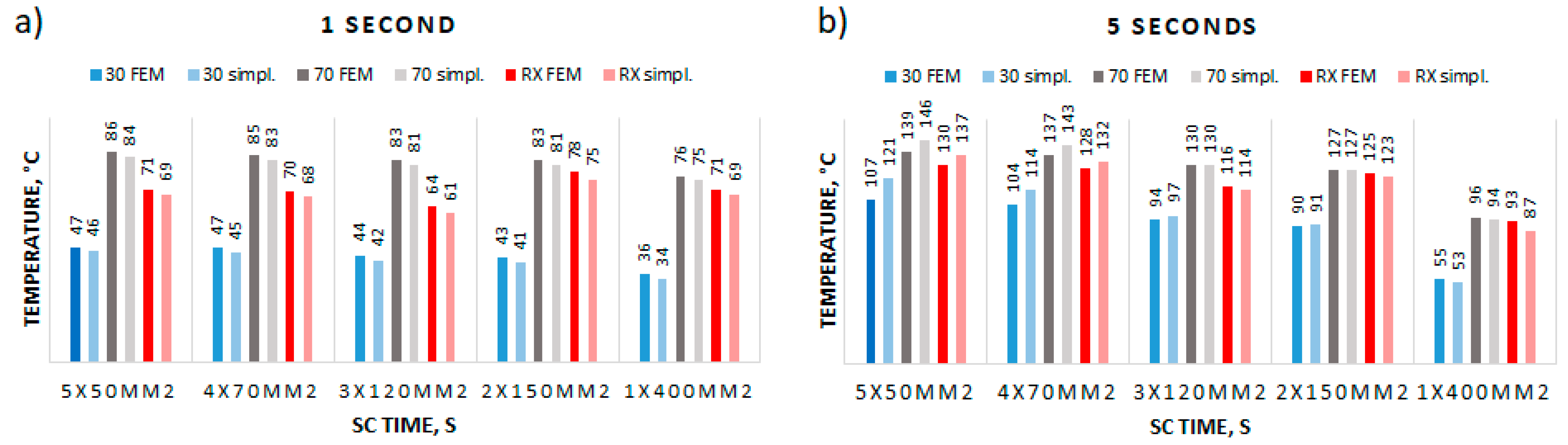
Formation	Case 1/30 °C SC Time, s					Case 1/70 °C SC Time, s
	1	2	3	4	5	1	2	3	4	5
5 × 50 mm2	47	63	78	93	107	86	100	113	126	139
4 × 70 mm2	47	62	76	91	104	85	99	112	125	137
3 × 120 mm2	44	57	69	82	94	83	95	107	119	130
2 × 150 mm2	43	55	67	78	90	83	94	105	116	127
1 × 400 mm2	36	41	45	50	55	76	81	86	91	96

,

Table 8. Temperature after SC depending on duration for case 2.

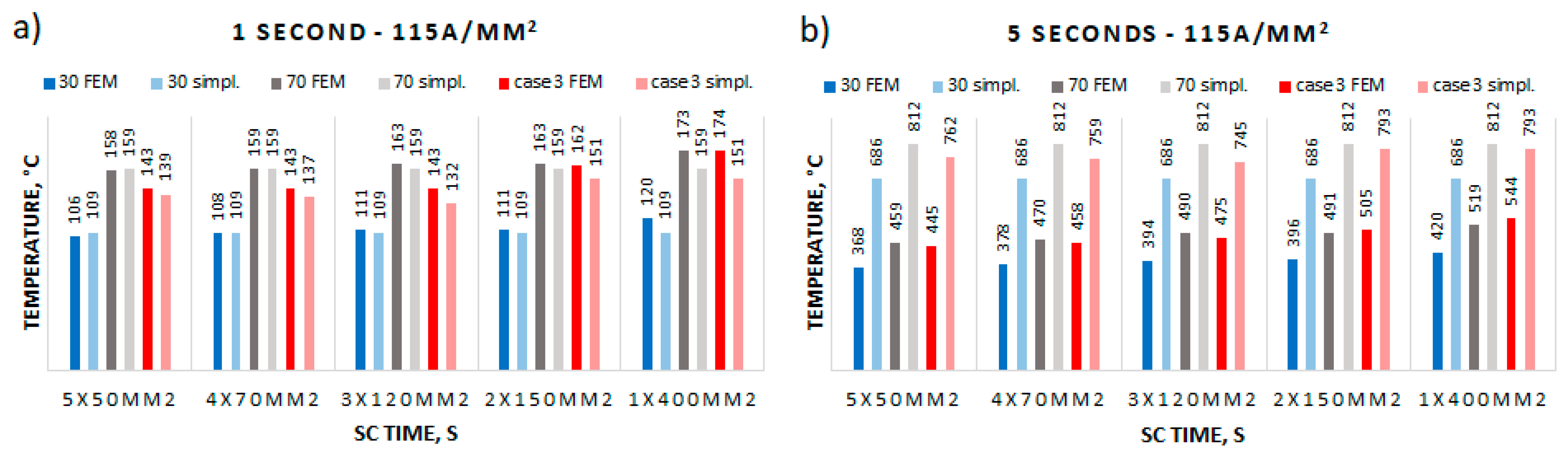
Formation	Case 2/30 °C SC Time, s					Case 2/70 °C SC Time, s
	1	2	3	4	5	1	2	3	4	5
5 × 50 mm2	106	176	242	306	368	158	238	315	388	459
4 × 70 mm2	108	179	248	314	378	159	241	320	396	470
3 × 120 mm2	111	185	256	326	394	163	248	331	411	490
2 × 150 mm2	111	185	257	327	396	163	248	331	412	491
1 × 400 mm2	120	196	272	347	420	173	262	349	434	519

and

Table 9. Temperature after SC depending on time duration for case 3.

Formation	Case 3/JRX SC Time, s					Case 3/Jd = 115 A/mm2 SC Time, s
	1	2	3	4	5	1	2	3	4	5
5 × 50 mm2	71	87	102	116	130	143	223	300	374	445
4 × 70 mm2	70	85	100	114	128	143	226	306	383	458
3 × 120 mm2	64	78	91	104	116	143	230	314	396	475
2 × 150 mm2	78	90	102	114	125	162	251	337	422	505
1 × 400 mm2	71	76	82	87	93	174	267	361	453	544

. First of all, it should be emphasised that case 2 is used in the calculations as a boundary condition according to the standard requirements. This is why such high temperatures are observed, especially for the 1 × 400 formation.

In the first case, it is visible that the highest temperatures occur in the smallest CSAs. The greater the cable, the lower the temperature increment (Figure 2 and Table 7 and

Table 10. Analytical calculation results of temperature after SC depending on time duration for case 1.

Formation	Case 1/30 °C SC Time, s					Case 1/70 °C SC Time, s
	1	2	3	4	5	1	2	3	4	5
5 × 50 mm2	46	64	82	101	121	84	99	114	130	146
4 × 70 mm2	45	61	78	96	114	83	97	112	127	143
3 × 120 mm2	42	55	69	83	97	81	93	105	117	130
2 × 150 mm2	41	53	65	78	91	81	92	103	115	127
1 × 400 mm2	34	39	44	48	53	75	79	84	89	94

). The reverse trend is observable in case 2, when the SC current density was set as a constant value of 115 A/mm². The highest temperatures for each SC time were for the 1 × 400 formation, and the lowest for the 5 × 50 (Figure 3). Both relationships from cases 1 and 2 are visible in the results of case 3. For a constant SC current density, trends are as in case 2, and for SC currents resulting from the assumed parameters of the cables and power system, the temperatures of the cable cores behave as in case 1 (Figure 4 and Table 9).

Taking into account an analytical method of the temperature calculation of the SC according to the Franz–Wiedemann law, the results are shown in Table 10 and

Table 11. Analytical calculation results of temperature after SC depending on time duration for case 3.

Formation	Case 3/JRX SC Time, s					Case 3/Jd = 115 A/mm2 SC Time, s
	1	2	3	4	5	1	2	3	4	5
5 × 50 mm2	69	85	102	119	137	139	245	380	549	762
4 × 70 mm2	68	83	99	115	132	137	244	378	546	759
3 × 120 mm2	61	74	87	100	114	132	237	370	536	745
2 × 150 mm2	75	86	98	110	123	151	261	400	574	793
1 × 400 mm2	69	73	78	83	87	151	261	400	574	793

for cases 1 and 3 and in Figure 3 for case 2. Generally, the results from FEA and the analytical method are convergent for very short faults, while for long ones (e.g., 5 s) the differences are the largest. It is necessary to underline that for a current density 115 A/mm², the core temperature in most cases exceeded the limit value of 160 °C and 140 °C for the cables greater than 300 mm². In case 1 (both initial temperatures) and case 3 (for resultant SC currents, RX case), there is no situation with a temperature growth over 160 °C. In the other cases the boundary values were exceeded significantly. Figure 5 depicts the results of the FEM calculations for chosen cases. In the FEM models, the number of elements in the computational mesh ranged from 12,248 (for the 1 × 400) to 17,716 (for the 5 × 50).

All the analyses were conducted using simulation models in FEMM software and the Franz–Wiedemann calculation method. As mentioned above, it is difficult to prepare such an energy-intensive laboratory bench under real conditions. However, in order to validate the adopted models, it is possible to use the manufacturer’s data of the time heating constant [27] and compare the results obtained from the simulation models. The values of the time heating constant were obtained using the methods given in [30]. These results are in

Table 12. Time heating constant for the investigated cables.

Cable Type	Time Heating Constant, s
	Manufacturer Value [27]	Simulation Value
50 mm2	350	343
70 mm2	426	409
120 mm2	616	610
150 mm2	727	745
400 mm2	1447	1455

.

The time heating constants are close to the values given by the manufacturer. Therefore, the models of these cables can be used in calculations of the temperature variations during SC.

4. Discussion

As can be seen, the results of cable heating during an SC are not easy to interpret with a universal rule which can be applied to any cable formation (as a possible alternative arrangement). Simplified methods that allow the cable core to be calculated using the Franz–Wiedemann law give satisfactory results only for relatively short fault durations. For small cable CSAs, this method coincides with FEA calculations, which are shown in Figure 6 and Figure 7. When the current density is not given as a constant value, as in case 2, but is a result of system and cable parameters, both methods give acceptable results. However, for high SC currents (so the current density as well), the simplified method gives much greater temperature values than the FEM model calculations. For 50 mm² cables, the difference reaches 353 °C for the SC lasting 5 s, which is definitely unacceptable. For the 1 s SC and constant current density, differences between the methods are relatively small, and only for the 1 × 400 formation in each calculating case does a temperature difference greater than 10 °C occur (the FEM gives higher temperatures than the simplified method). At first glance, it can be seen that the simplified method results in the same temperature after SC current flow for all cable arrangements. The FEM refers to each formation individually, so the results are different. Generally, when the current density for each cable is the same and equal to 115 A/mm², the temperatures of the cores increase as the CSA grows. From these analyses emerges a conclusion that the simplified method based on the Franz–Wiedemann law is appropriate only in a given range of current densities and times. The issue of the time is fully understandable, because this method can be adopted only for adiabatic processes. When heat transfer occurs in the object under analysis, this method can no longer be used.

From the conducted studies, conclusions can also be drawn referring to the dependencies on temperature and power losses. When the current density is constant for all cable formations, the power losses resulting from Joule heat may be constant as well (it depends on the resistance variation). However, when even the unitary power losses (power losses divided through the CSA, W/mm²) are constant, the cable can heat differently. And in this case the dependency on the specific power loss per unit length of the conductor circuit can be observed. The greater the specific power loss divided through the conductor circuit, the higher the conductor temperature. Thus, the larger cables achieved higher temperatures, despite the fact that the current and power loss density was equal to that of the smaller cables. This is an important observation from this research. In the simplified method, this issue was omitted and only the current density (so approximately also power losses according to the CSA) was a main parameter influencing the temperature of the cable. And therefore, in case 2 each arrangement temperature was the same, independently of the formation and SC duration.

Disregarding the methods of cable temperature calculation, it is important to notice that in case 2 each cable formation fault with a duration longer than 1 s resulted in temperatures above 160 °C (and 140 °C for 1 × 400). A similar situation may be highlighted in case 3 for current density of 115 A/mm². For SCs longer than 1 s and for such a high current density, the temperature increments are acceptable, however, in the case of a 1 s SC for formations 3 × 120, 2 × 150, and 1 × 400 (case 2) the maximal permissible temperatures are exceeded. An analogous situation is in case 3 with 115 A/mm² for 2 × 150 and 1 × 400.

Based on the calculations carried out for the assumed cases, it is possible to verify how the cables heat up during the SC. Obviously, this manuscript only presents chosen cases for the assumed cable layouts, but in real installations in industry other cases can be found depending on the parameters of the power system and installation. Because there are so many possible cases, the case of a current density 115 A/mm² was used.

The performed studies allow the preparation of further research in order to obtain calculation methods that take into account the effects of heating and their impact on the SC current values, power losses, and resistivity changes. These aspects are intuitively known in the power engineering environment, however, some situations can be found that are not verified by engineers. As an example, the following situation can be given: in a working installation an SC occurred and it was switched off after 1 s. Then, after some time, another fault occurred. The second SC has completely different conditions and this situation may affect the safety and correct operation of the protection devices.

The temperature increments shown in Figure 2, Figure 3 and Figure 4 indicate that the initial temperature has a great influence on the SC current value. It is visible that in case 1 the temperature increases more significantly for a lower initial temperature. Such a dependency is observable for small CSAs, and for the 1 × 400 formation the cable temperature growth is greater for an initial temperature of 70 °C. It should be underlined that the assumed calculations do not take into account the temperature increase and its effect on the resistance change. In further research, it is planned to develop an algorithm allowing consideration of temperature variations to obtain a more accurate calculation method.

The different cable formations that can be chosen to supply any load have advantages and disadvantages. In a system consisting of several cables connected in parallel, the temperature rise is the highest (case 1 and case 3 RX). This is a result of an equivalent resistance of each cable formation and system parameters, which result in a different SC current value. For an assumed constant current density, the highest temperature increments occur for the cables with the largest CSA.

All calculations are theoretical. The temperatures of the cable conductors reach very high values, especially for long-lasting SCs. Under these conditions (temperatures of 700 or 800 °C from Figure 7), the insulation and outer sheath would be damaged and the cable would no longer be used. The problem of SC prevention is a separate issue that is not investigated in this manuscript. However, such high temperatures of the cable conductors indicate what could happen if a very high SC current flows in an electrical circuit and the protective devices react slowly (with a maximum reaction time of 5 s). For the assumed cases and high temperatures, there is a risk of fire [31].

The research presented in this manuscript refers only to calculation methods and the effects on cable temperatures. It should be emphasised that real-life tests for such problems as short circuits with variable and adjustable current values are very hard to implement at the laboratory scale, especially for large-CSA cables. It is difficult to achieve current values measured in tens of thousands of amperes. The second issue according to the theoretical research and its laboratory validation—it is impossible to measure the temperature of the cable conductor continuously without any instrument interference, which may additionally change the parameters of measured objects, especially for fast phenomena such as SCs.

5. Conclusions

The conducted research considering different cable arrangements and their effects on the short-circuit currents and the cable heating process allow the verification of how some of the negative effects can be reduced by changing the cable layout. In modern installations, it is common practice to use several cables connected in parallel instead of a single cable per phase. And, therefore, it is necessary to verify how these formations can perform during faults.

In this manuscript, two computational methods were compared. The first used the FEM and the second one was based on the Franz–Wiedemann law as a simplified method. The results were in some ranges convergent and in some ranges unacceptable. Based on the results obtained, it is possible to develop further research in order to obtain an empirical analytical computational method to perform a rapid thermal analysis of cables under short-circuit conditions. This is a consequence of the results obtained in the simplified method for an assumed constant current density. In such cases, each formation should have the same temperatures of the cable conductors, which is a serious shortcoming of this method. In addition, the simplified method gave relatively high temperature values for high short-circuit currents, which also indicates the inaccuracy of this method.

References

- IEC 60364-5-52:2009; Low-Voltage Electrical Installations—Part 5-52: Selection and Erection of Electrical Equipment—Wiring systems. International Standard: Geneva, Switzerland, 2009.
- Fangrat, J.; Kaczorek-Chrobak, K.; Papis, B.K. Fire Behavior of Electrical Installations in Buildings. Energies 2020, 13, 6433. [Google Scholar] [CrossRef]
- IEC TR 62095:2003; Electric Cables-Calculations for Current Ratings-Finite Element Method. International Standard: Geneva, Switzerland, 2003.
- Rerak, M.; Ocłoń, P. Thermal analysis of underground power cable system. J. Therm. Sci. 2017, 26, 465–471. [Google Scholar] [CrossRef]
- Ocłoń, P.; Pobędza, J.; Walczak, P.; Cisek, P.; Vallati, A. Experimental Validation of a Heat Transfer Model in Underground Power Cable Systems. Energies 2020, 13, 1747. [Google Scholar] [CrossRef]
- Anders, G.J. Rating of Electric Power Cables: Ampacity Computations for Transmission, Distribution, and Industrial Application; IEEE PRESS: New York, NY, USA, 1997. [Google Scholar]
- Bates, C.; Malmedal, K.; Cain, D. Cable ampacity calculations: A comparison of methods. IEEE Ind. Appl. 2016, 52, 112–118. [Google Scholar] [CrossRef]
- Wang, P.-Y.; Ma, H.; Liu, G.; Han, Z.-Z.; Guo, D.-M.; Xu, T.; Kang, L.-Y. Dynamic thermal analysis of high-voltage power cable insulation for cable dynamic thermal rating. IEEE Access 2019, 7, 56095–56106. [Google Scholar] [CrossRef]
- Zhan, Q.; Ruan, J.; Tang, K.; Tang, L.; Liu, Y.; Li, H.; Qu, X. Real-time calculation of three cable conductor temperature based on thermal circuit model with thermal resistance correction. J. Eng. 2019, 16, 2036–2041. [Google Scholar] [CrossRef]
- Wang, J.; Liang, Y.; Ma, C. A novel transient thermal circuit model of buried power cables for emergency and dynamic load. Energy Rep. 2023, 9 (Suppl. S1), 963–971. [Google Scholar] [CrossRef]
- Olsen, R.S.; Holboll, J.; Gudmundsdóttir, U.S. Dynamic Temperature Estimation and Real Time Emergency Rating of Transmission Cables. In Proceedings of the 2012 IEEE Power and Energy Society General Meeting, San Diego, CA, USA, 22–26 July 2012; pp. 1–8. [Google Scholar] [CrossRef]
- Luo, L.; Cheng, X.; Zong, X.; Wei, W.; Wang, C. Research on Transmission Line Loss and Carrying Current Based on Temperature Power Flow Model, 3rd International Conference on Mechanical Engineering and Intelligent Systems; Atlantis Press: Amsterdam, The Netherlands, 2015; pp. 120–127. [Google Scholar] [CrossRef]
- Sarajcev, I.; Majstrovic, M.; Medic, I. Calculation of Losses in Electric Power Cables as the Base for Cable Temperature Analysis; WIT, Transactions on Engineering Sciences; WIT Press: Waterford, Ireland, 2020; Volume 27, pp. 529–537. [Google Scholar]
- Wang, X.W.; Zhao, J.P.; Zhang, Q.G.; Lv, B.; Chen, L.C.; Zhang, Y.; Yang, J.H. Real-time Calculation of Transient Ampacity of Trench Laying Cables Based on the Thermal Circuit Model and the Temperature Measurement. In Proceedings of the 2019 IEEE 8th International Conference on Advanced Power System Automation and Protection (APAP), Xi’an, China, 21–24 October 2019; pp. 1647–1651. [Google Scholar] [CrossRef]
- Kacejko, P.; Machowski, J. Short Circuits in the Electroenergetic System; WNT: Warszawa, Poland, 2020. (In Polish) [Google Scholar]
- Mamcarz, D.; Albrechtowicz, P.; Radwan-Pragłowska, N.; Rozegnał, B. The Analysis of the Symmetrical Short-Circuit Currents in Backup Power Supply Systems with Low-Power Synchronous Generators. Energies 2020, 13, 4474. [Google Scholar] [CrossRef]
- Rozegnał, B.; Albrechtowicz, P.; Mamcarz, D.; Radwan-Pragłowska, N.; Cebula, A. The Short-Circuit Protections in Hybrid Systems with Low-Power Synchronous Generators. Energies 2021, 14, 160. [Google Scholar] [CrossRef]
- Wu, Y. Numerical Simulation and Characteristics Test of Temperature Field under Short-circuit Fault. In Proceedings of the 2017 2nd International Conference on Modelling, Simulation and Applied Mathematics (MSAM2017), Advances in Intelligent Systems Research, Bangkok, Thailand, 26–27 March 2017. [Google Scholar] [CrossRef]
- Hao, J.; Zhou, J.; Wang, Y. Thermal Stability Analysis and Design for Electrical Product in Short-Circuit Fault. Elektron. Ir Elektrotechnika 2022, 28, 18–26. [Google Scholar] [CrossRef]
- Vikharev, A.P. Calculation of the Admissible Short Circuit Current for the Protected Wires of an OHL. Power Technol. Eng. 2018, 52, 357–360. [Google Scholar] [CrossRef]
- Brakelmann, H.; Anders, G.J. Transient Thermal Response of Multiple Power Cables With Temperature Dependent Losses. IEEE Trans. Power Deliv. 2021, 36, 3937–3944. [Google Scholar] [CrossRef]
- Brakelmann, H.; Anders, G.J. Ampacity Calculations of Underground Power Cables With End Effects. IEEE Trans. Power Deliv. 2023, 38, 1968–1976. [Google Scholar] [CrossRef]
- Riba, J.-R. Analysis of formulas to calculate the AC resistance of different conductors’ configurations. Electr. Power Syst. Res. 2015, 127, 93–100. [Google Scholar] [CrossRef]
- Chaganti, P.; Yuan, W.; Zhang, M.; Xu, L.; Hodge, E.; Fitzgerald, J. Modelling of a High-Temperature Superconductor HVDC Cable Under Transient Conditions. IEEE Trans. Appl. Supercond. 2023, 33, 5400805. [Google Scholar] [CrossRef]
- Albrechtowicz, P.; Szczepanik, J. The analysis of the effectiveness of standard protection devices in supply systems fed from synchronous generator sets. In Proceedings of the 2018 International Symposium on Electrical Machines (SME): SME 2018, Andrychów, Poland, 10–13 June 2018; pp. 1–5. [Google Scholar]
- Lubośny, Z. Virtual Inertia in Electric Power Systems. Autom. Elektr. Zaklocenia 2020, 11, 1. [Google Scholar] [CrossRef]
- NKT Group. NKT Cable Calatogue, Low Voltage Cables and Wires; NKT S.A.: Warszowice, Poland, 2017. [Google Scholar]
- IEC 60502-1:2021; Power Cables with Extruded Insulation and their Accessories for Rated Voltages from 1 kV (Um = 1.2 kV) up to 30 kV (Um = 36 kV)—Part 1: Cables for Rated Voltages of 1 kV (Um = 1.2 kV) and 3 kV (Um = 3.6 kV). International Standard: Geneva, Switzerland, 2021.
- IEC 60724:2000; Short-Circuit Temperature Limits of ELECTRIC Cables with Rated Voltages of 1 kV (Um = 1.2 kV) and 3 kV (Um = 3.6 kV). International Standard: Geneva, Switzerland, 2000.
- Lejdy, B.; Skibko, Z. Determine of thermal time-constant based on temperature measuring. In Pomiary Automatyka Kontrola; Wydawnictwo PAK: Warszawa, Poland, 2010; Volume 56, pp. 143–145. [Google Scholar]
- Chybowski, R.; Jaskółowski, W.; Kustra, P. Wpływ grubości tynku na funkcjonalność pojedynczego przewodu elektrycznego poddanego oddziaływaniu promieniowania cieplnego. Zesz. Nauk. SGSP/Szkoła Główna Służby Pożarniczej 2012, 43, 5–12. [Google Scholar]