Multivariate Deep Learning Long Short-Term Memory-Based Forecasting for Microgrid Energy Management Systems

Abstract

In the scope of energy management systems (EMSs) for microgrids, the forecasting module stands out as an essential element, significantly influencing the efficacy of optimal solution policies. Forecasts for consumption, generation, and market prices play a crucial role in both day-ahead and real-time decision-making processes within EMSs. This paper aims to develop a machine learning-based multivariate forecasting methodology to account for the intricate interplay pertaining to these variables from the perspective of day-ahead energy management. Specifically, our approach delves into the dynamic relationship between load demand variations and electricity price fluctuations within the microgrid EMSs. The investigation involves a comparative analysis and evaluation of recurrent neural networks’ performance to recognize the most effective technique for the forecasting module of microgrid EMSs. This study includes approaches based on Long Short-Term Memory Neural Networks (LSTMs), with architectures ranging from Vanilla LSTM, Stacked LSTM, Bi-directional LSTM, and Convolution LSTM to attention-based models. The empirical study involves analyzing real-world time-series data sourced from the Australian Energy Market (AEM), specifically focusing on historical data from the NSW state. The findings indicate that while the Triple-Stacked LSTM demonstrates superior performance for this application, it does not necessarily lead to more optimal operational costs, with forecast inaccuracies potentially causing deviations of up to forty percent from the optimal cost.

1. Introduction

Multivariate Deep Learning Forecasting (MVDLF) has emerged as a technique in the area of microgrid energy management systems, addressing the challenges of dual prediction of price and demand. By leveraging vast amounts of historical and real-time data, MVDLF models can capture complex, non-linear relationships between multiple variables. Incorporating supplementary electrical load-related features in multivariate input configurations frequently enhances forecasting accuracy. Weather conditions, which load data are particularly sensitive to, are among the most essential external factors affecting the load. Additionally, factors such as electricity prices, weekdays, public holidays, economic indicators, and demographic information play a significant role in influencing the load [1]. The multivariate forecasting capability is crucial for optimizing energy distribution, reducing operational costs, and enhancing the reliability and sustainability of microgrids. The application of MVDLF not only facilitates more efficient energy management but also supports the integration of renewable energy sources, contributing to the broader goals of energy efficiency and environmental conservation.

Generally, data forecasting in energy management systems (EMSs) can typically be divided into four categories based on the forecast interval length. Very short-term forecasting predicts data for a few minutes. Short-term forecasting covers periods from one day to one week. In a longer timescale, medium-term forecasting spans from over one week to a couple of months. Finally, long-term forecasting extends beyond one year [2,3]. The short-term forecasting for energy management problem has been addressed using various methods, broadly categorized into traditional methods and computational intelligence methods [2]. Deep learning frameworks have recently garnered significant attention. Unlike shallow learning, deep learning usually employs multiple hidden layers, enabling models to grasp intricate non-linear patterns more effectively. Among these frameworks, recurrent neural networks (RNNs) stand out for their robust ability to capture non-stationary and long-term dependencies in forecasting horizons [4]. Neural networks acquire knowledge through training to anticipate forthcoming values using pertinent input data. These networks offer numerous advantages, such as adaptive learning, seamless integration with existing networks or technologies, fault tolerance, and real-time operation. Their capability to generalize and handle non-linearities in intricate ambiences makes these neural networks particularly appealing for applications in load forecasting [5]. In this context, a deep neural network appears to be a type of artificial neural network distinguished by having more layers than the standard three-layer architecture of a multilayer perceptron. This deeper structure significantly enhances the neural network’s ability to abstract and learn complex features [6]. However, these networks face challenges such as vanishing gradients. To mitigate this issue and enhance the performance of RNNs, variants such as Gated Recurrent Units (GRUs) and Long Short-Term Memory (LSTM) have emerged and have been proven effective in long-term horizon forecasting [7,8].

The application of LSTM neural networks, which are the main focus of this study, within energy management systems is not limited to pure data forecasting. An integrated prediction into energy storage management is developed in [9] to minimize the operational cost of energy systems. The developed model’s hyperparameters are optimized by an evolutionary algorithm. Heuristic algorithms are widely used for hyperparameter optimization. For example, a genetic algorithm combined with particle swarm optimization is utilized in [10] to optimize an LSTM network for energy management problems considering demand response initiatives. Regarding feature selection for load forecasting, a technique according to mutual information is employed by authors in [11], along with an error minimization using evolutionary algorithms.

Single forecasting models have limitations in achieving high precision consistently, as each model has its strengths and weaknesses. To mitigate the shortcomings inherent in individual models, numerous combined forecasting models have been proposed, offering improved forecasting performance [12]. Researchers leverage the strengths of combined models to improve prediction accuracy and enhance system performance. The combination of convolutional neural networks (CNNs) and LSTM networks has been extensively used in prediction tasks. CNNs excel at capturing local trends and scale-invariant features, and are particularly effective when neighbouring data points exhibit robust interrelationships. They are particularly effective at extracting patterns of local trends from load data across neighbouring hours [2,13]. The study in [14] introduces a two-phased framework for short-term electricity load forecasting, comprising a data cleansing phase followed by a residual CNN integrated with a Stacked LSTM architecture. The combination of CNNs and LSTM networks is investigated in [13] for load demand forecasting in energy systems. The authors of [15] also utilize the CNN layer for extracting the influential features for LSTM-based short-term load forecasting. Moreover, the combination of Bi-directional LSTM with an attention mechanism is investigated in [16] to predict electricity load and price using a hybrid method. These studies, however, neglect the correlation between load and price, which matters in energy management problems. Also, the considerations of microgrid energy management should be taken into account to analyze the impacts.

To the best of the authors’ knowledge, there is no investigation on the effect of different LSTM architectures on the optimal operational cost of microgrid energy management. This paper explores and compares various architectures of LSTM networks. These include the Vanilla LSTM, which represents the basic form of LSTM. We also explore the Stacked LSTM configuration, where multiple LSTM layers are sequentially stacked to enhance feature learning. The Bi-LSTM architecture leverages information from both forward and backward states of the time-series data to improve predictive accuracy. Additionally, we examine the attention-based LSTM, which selectively focuses on specific, randomly chosen segments of the input sequence to refine predictions. Finally, our study incorporates the CNN-LSTM model, combining convolutional neural network layers with LSTM layers to capture spatial and temporal dependencies of data points effectively. To evaluate the accuracy’s impact of the energy management optimal solution, a mathematical model of a renewable-based microgrid equipped with a battery energy storage system is also developed in this paper.

The remainder of this paper is structured as follows: Section 2 formulates the microgrid energy management problem and identifies the key factors influencing optimal decision-making. Section 3 introduces the proposed multivariate deep learning approach for forecasting electricity load demand and prices. The study’s findings are detailed in Section 4, with the conclusion provided in Section 5.

2. Proposed Energy Management Framework

2.1. Microgrid Energy Management Problem

The schematic microgrid illustrated in Figure 1 includes conventional generation units (CGUs), battery energy storage systems (BESs), and photovoltaic generation units (PVs) collectively designed to meet specific load requirements. The energy management system (EMS) is tasked with managing the generation schedule and interactions with the grid. As illustrated in this figure, data on price, load demand, battery energy storage systems (BESs), and generation availability, along with weather and calendar information, should be collected and transmitted to the EMS through the monitoring system. The EMS uses these data to forecast the necessary variables for the decision-making process. In this model, price data and load demand data are treated as forecasted inputs. The system model is then employed to calculate the optimized operational cost and determine the operational schedules for generation facilities, BESs, and energy exchange with the grid. The EMS relies on forecasted electricity market prices and load demand data to generate day-ahead hourly schedules for power generation and manage the state of charge (SoC) of BESs. The system is modelled as a single-node microgrid to evaluate the performance of the EMS using LSTM-based forecasting for input variables.

The mathematical formulation for energy management is detailed below. Equation (1) defines the objective function governing the optimization of operational strategies. It aims to minimize costs while ensuring a reliable power supply. This function incorporates factors such as exchange-related expenses, generation costs, and operational costs of BESs as denoted in (2) to achieve optimal economic performance. This equation calculates the cost of BESs which refers to the battery degradation stemming from charging or discharging. The cost incurred when the battery system remains unused during periods of zero charging or discharging, where the charging rate is also zero, is determined by the intercept ${\beta }_j^{BES}$. In this formulation, the binary variables (${\lambda }_h^{imp}, {\lambda }_h^{exp}$) help the optimization process enable or disable the microgrid external transactions.

$$OF:\hspace{0.17em}\hspace{0.17em}\min {\displaystyle \sum _{h=1}^H\left\{\begin{array}{l}({\mathit{Cost}}^{\mathit{exchange}}+{\displaystyle \sum _{i=1}^{CGU}Cos{t}_i^{CGU}}\\ +{\displaystyle \sum _{j=1}^{BES}Cos{t}_j^{BES,ch/dch}}+{\displaystyle \sum _{k=1}^{PV}Cos{t}_k^{PV}}\end{array}\right\}}$$

(1)

$$\min {\displaystyle \sum _{h=1}^H\left\{\begin{array}{l}\left({\lambda }_h^{imp}.E_{m,h}^{imp}.{\phi }_h^{imp}-{\lambda }_h^{exp}.E_h^{exp}.{\phi }_h^{exp}\right)\\ +{\displaystyle \sum _{i=1}^{CGU}\left(a_i^{CGU}{(E_{i,h}^{CGU})}^2+b_i^{CGU}(E_{i,h}^{CGU})+c_i^{CGU}\right)}\\ +{\displaystyle \sum _{j=1}^{BES}\left({\alpha }_j^{BES}{(E_{j,h}^{BES})}^2+{\beta }_j^{BES}\right)+{\displaystyle \sum _{k=1}^{PV}{\sigma }_k.E_{k,h}^{PV}}}\end{array}\right\}}$$

(2)

The objective function is subject to a series of constraints for the sake of system stability and balancing. The optimization model for CGUs must adhere to constraints (3) and (4) governing minimum and maximum generation capacities, as well as ramp rate limits. Furthermore, the operational cost of renewable generation, specifically the solar PV system, represented in (2), is determined by a constant nominal coefficient multiplied by the power output during its operational periods.

$$P_{i,\min }^{CGU}\le E_{i,h}^{CGU}\le P_{i,max}^{CGU}$$

(3)

$$E_{i,h-1}^{CGU}-R_i^{CGU}\le E_{i,h}^{CGU}\le E_{i,h-1}^{CGU}+R_i^{CGU}$$

(4)

To limit the amount of sending or receiving electricity to or from the upstream main grid,

$${\lambda }_h^{imp}\cdot E_h^{imp}\le P_{\max }^{imp}$$

(5)

$${\lambda }_h^{exp}\cdot E_h^{exp}\le P_{\max }^{exp}$$

(6)

In this study, the modelling of battery systems integrates essential parameters such as state of charge (SoC), charging and discharging rates, efficiency, and capacity constraints. These parameters are typically formulated mathematically based on fundamental principles and empirical data. Moreover, the operational behaviour of batteries within the microgrid EMS is governed by constraints of capacity limits, charge/discharge rates, and maximum/minimum SoC levels, as outlined in Equations (7) to (10). These constraints ensure optimal battery performance, extend battery lifespan and prevent simultaneous charging and discharging. Notably, values above zero indicate discharging, while values below zero indicate charging, reflecting the BES’s role as an energy source rather than a load. Additionally, Equation (10) computes the remaining charge or SoC for the subsequent hour.

$$P_{j,\max }^{BES,ch}\le E_{j,h}^{BES}\le P_{j,max}^{BES,dch}$$

(7)

$${\gamma }_h^{ch}+{\gamma }_h^{dch}=1$$

(8)

$$So{C}_{\mathrm{j},\min }\le So{C}_{\mathrm{j},h}\le So{C}_{\mathrm{j},\max }$$

(9)

$$So{C}_h=\left(\begin{array}{l}So{C}_{h-1}+{\eta }_{\mathrm{j},ch}^{BES}({\gamma }_h^{ch}{\displaystyle \frac{E_{j,h}^{BES}}{Ca{p}_j^{BES}}})\\ -{\displaystyle \frac{1}{{\eta }_{\mathrm{j},dch}^{BES}}}({\gamma }_h^{dch}{\displaystyle \frac{E_{j,h}^{BES}}{Ca{p}_j^{BES}}})\end{array}\right)$$

(10)

The objective function described above dynamically adjusts to varying energy demands and generation especially renewable energy availability, facilitating efficient resource utilization while adhering to operational constraints. Therefore, maintaining the power balance between generation and consumption shown by (11) is of great importance, accounting for energy exchanges with the grid.

$$\begin{array}{l}\left(E_h^{Load}+{\gamma }_h^{ch}{\displaystyle \sum _{j=1}^{BES}{E}_{j,h}^{BES,ch}}+{\lambda }_{m,h}^{exp}\cdot E_{m,h}^{exp}\right)=\\ \left(\begin{array}{l}{\lambda }_{m,h}^{imp}\cdot E_{m,h}^{imp}+{\gamma }_h^{dch}{\displaystyle \sum _{j=1}^{BES}{E}_{j,h}^{BES,dch}}\\ +{\displaystyle \sum _{k=1}^{PV}{E}_{k,h}^{PV}}+{\displaystyle \sum _{i=1}^{CGU}{E}_{i,h}^{CGU}}\end{array}\right)\end{array}$$

(11)

To mitigate opportunistic behaviour by the EMS, such as importing electricity in a time step to export it for profit in the immediate next step, and to prevent simultaneous importing and exporting of electricity, constraints (12) and (13) are also enforced.

$${\phi }_h^{exp}\le {\phi }_h^{imp}\hspace{0.17em}\hspace{0.17em}\hspace{0.17em}\forall \hspace{0.17em}h\in H$$

(12)

$${\lambda }_h^{imp}+{\lambda }_h^{exp}=1\hspace{0.17em}\hspace{0.17em}\hspace{0.17em}\forall \hspace{0.17em}h\in H$$

(13)

2.2. Influential Factors on Optimal Decisions

Optimal decisions in energy management are significantly influenced by various forecasted factors, including electricity demand and price. Electricity demand is shaped by a combination of elements such as the prevailing electricity price, which can either incentivize or dissuade consumption. Weather conditions also play a critical role, as temperature extremes can increase heating or cooling needs. Seasonal variations, with different months of the year affecting usage patterns due to changing daylight hours and climatic conditions, are important as well. Additionally, the day of the week influences demand, with weekdays generally exhibiting higher industrial and commercial usage compared to weekends. Finally, the time of day is a crucial factor, as peak hours in the morning and evening see heightened residential and commercial activity, impacting overall demand. These factors must be meticulously forecasted and integrated into energy management strategies to optimize resource allocation and minimize costs. Given the complexity and variability of factors influencing electricity demand and price, such as weather conditions, seasonal trends, and daily usage patterns, a sophisticated forecasting approach is essential. Advanced methods like machine learning and time-series analysis can accurately predict these fluctuations, enabling better resource utilization and financial management.

3. Multivariate Deep Learning Forecasting

The majority of research in energy forecasting has traditionally focused on univariate forecasting methods. These methods estimate marginal predictive densities for individual time series under the assumption that the time series are conditionally independent in high-dimensional scenarios. However, this approach neglects the complex temporal, spatial, and cross-lagged correlations present in microgrid systems, such as the relationship between successive electricity market prices, and the lagged impact of weather conditions on load profiles. Ignoring these correlations can lead to suboptimal decision-making in microgrid operations, especially when dealing with extended optimization periods. Conversely, by simultaneously considering multiple variables, it is possible to capture and utilize consistent patterns, leading to more accurate forecasts and cost reductions. Consequently, there is growing interest in multivariate forecasting models, which can incorporate spatiotemporal and cross-lagged correlations within a single global model [17]. In this research paper, a multivariate forecasting approach for energy management systems is adopted, utilizing multi-output machine learning models to predict two key response variables (models’ output), i.e., electricity demand and price, simultaneously. This approach recognizes the complex interdependencies between demand and price, which are influenced by a range of independent variables, serving as the model’s inputs.

The application of deep learning models enables effective modelling of temporal dependencies in multivariate forecasting, facilitating feature extraction and dimensionality reduction [18]. More specifically, employing multivariate forecasting using LSTM networks for demand and price predictions is highly justified due to the ability of LSTMs to capture complex temporal dependencies and relationships among multiple influencing factors. LSTM networks excel at handling time-series data with long-term dependencies, making them well suited for predicting electricity demand and price, which are influenced by various interrelated factors including weather conditions, seasonality, weekday, and time of day. By incorporating these multiple variables, LSTMs can learn the intricate patterns and correlations that simpler models might miss, leading to more accurate and reliable forecasts. This paper aims to compare different LSTM architectures to examine the impact of forecast errors on optimal costs. By identifying the most accurate architecture, the study seeks to help operators manage system operational costs more effectively.

3.1. Data Processing Methodology

The process is carried out in four general steps: accumulation and preparation of historical demand, price and meteorological data; data pre-processing; data forecasting; and post-processing data analysis. Figure 2 provides a detailed depiction of this procedure. Once processed, the forecasted data are fed into the optimization module to facilitate optimal decision-making. Accurate load forecasting requires the use of feature engineering to determine the relevant input variables [1]. The input generation or consumption data require preparation and pre-processing to eliminate redundant and irrelevant features for two primary reasons: first, redundant features do not contribute additional information and only prolong the training process; second, irrelevant features act as outliers and do not provide meaningful information. Moreover, data pre-processing aids in removing outliers, handling missing or redundant samples, and enhancing prediction accuracy. The data statistics before and after pre-processing are calculated and presented in

Table 1. The data statistics before and after pre-processing.

	(a) Before Outlier Resolution		(b) After Outlier Resolution
	Demand (MW)	Price (AUD)	Demand (MW)	Price (AUD)
count	17,519	17,519	17,519	17,519
mean	7550.56	72.42	7514.49	52.67
std	1246.55	220.91	1186.27	21.97
min	4316.63	−1000	4316.63	−14.47
25%	6642.59	35.49	6642.59	35.59
50%	7402.64	49.24	7402.64	50.05
75%	8219.87	68.83	8185.41	69.90
max	12,863.76	9420.84	11,286.96	118.85

. In addition, normalization is essential to scale the dependent and independent variables uniformly, and it should be performed prior to optimizing the machine learning model.

3.2. Demand and Price Interplay

In practical applications, the data acquired often have high dimensionality, which can make training deep learning models challenging. To overcome this, dimensionality reduction techniques are applied [19]. One common approach is the Pearson correlation coefficient (PCC), which evaluates the linear correlation between two continuous variables and helps identify the most correlated data. To visualize the correlation among different features within the dataset, monthly data points are presented in Figure 3. To assess the relationship between these features and demand, Figure 4 includes a heatmap illustrating the correlations of demand with price, temperature, hour of the day, day of the week, weekday type, and month within the dataset. As shown in this figure, demand and price exhibit a relatively high correlation, with a value of 0.46. In the provided dataset, temperature shows less correlation than expected, due to the low variation in temperature across the entire area on average. The hour of the day and the type of weekday also show a significant correlation with demand, indicating that demand fluctuates throughout the day and week, with certain periods experiencing higher demand. Regarding price, the strongest correlation is with demand, followed by the month of the year, suggesting that seasonal variations significantly influence electricity prices. Interestingly, the weekday and weekend features have a correlation of 0.79, which can be attributed to the distinction between weekend days and weekdays. It is important to note that zero values in Figure 4 indicate no correlation, such as between hour and weekday, while positive and negative values represent direct and inverse correlations, respectively.

Electricity prices frequently display periodic trends, making historical prices, such as those from one week or several months prior, valuable input variables for predictive models. Additionally, market prices reflect the balance between supply and demand [20]. Each cell in the heatmap denotes the strength and direction of the correlation, whether positive or negative, computed using PCC, which is deemed more appropriate than alternative methods such as Spearman’s Rank Correlation and Kendall’s Tau for this analysis. PCC measures the degree of linear relationship between two variables, ranging from −1 to 1, where a value of 1 signifies a complete positive linear relationship, while −1 indicates a complete negative linear relationship, and 0 indicates no linear relationship between the variables [21]. In this study, the demand and price dataset from NSW, Australia, is utilized for correlation analysis and the calculations are based on the Pearson correlation coefficient, defined in (14) [19].

$$r={\displaystyle \frac{{\sum }_{i=1}^n\left(V_i-\overline{V}\right)\left(W_i-\overline{W}\right)}{\sqrt{{\sum }_{i=1}^n{\left(V_i-\overline{V}\right)}^2}\sqrt{{\sum }_{i=1}^n{\left(W_i-\overline{W}\right)}^2}}}$$

(14)

where r denotes the Pearson correlation coefficient between variables V and W. V_i and W_i are individual data points, and $\overline{V}$ and $\overline{W}$ represent their respective means.

3.3. LSTM Networks for Multivariate Forecasting

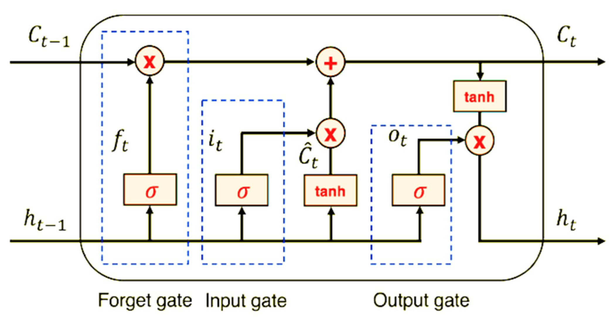
LSTM-based forecasting methods have significantly advanced time-series prediction by effectively handling sequential data and capturing long-term dependencies. The Vanilla LSTM, or the standard LSTM model, employs a simple yet powerful architecture with gates that regulate the flow of information, making it adept at learning temporal patterns and mitigating the vanishing gradient problem. Figure 5 illustrates the common LSTM cell architecture where C_t is the memory cell’s internal state, h_t is the hidden state, and it and O_t represent the input gate and output gate, respectively. The specific mechanism and formulation used in LSTM architectures are detailed in [22].

The Stacked LSTM builds on the standard LSTM model by layering multiple LSTM networks, enabling the model to learn more complex representations and hierarchical features, thereby enhancing prediction accuracy for intricate time series. The stacked configuration in RNNs is based on the idea of deepening the network by layering multiple recurrent hidden states on top of each other. This approach allows each layer’s hidden state to operate at different timescales, potentially improving the model’s ability to capture complex temporal patterns [23]. A stacking approach with various numbers of hidden layers is presented in [24] to predict electrical energy demand.

Bi-directional LSTM expands on the Vanilla LSTM by processing data in both forward and backward directions. This dual processing allows the network to learn from past and future values, making it particularly effective for forecasting electricity demand, which relies heavily on historical data [3]. However, unidirectional LSTM networks are limited to learning the current state using information from past states only, without considering future data [25]. Therefore, the dual approach provides a comprehensive understanding of the sequence context, improving the accuracy of predictions in tasks where future information is relevant.

The recent advancements in AI technology have significantly improved combinational deep learning algorithms, such as convolutional neural networks (CNNs) and Long Short-Term Memory (LSTM) networks. A convolutional neural network (CNN) is a specialized type of artificial neural network designed to process and analyze data with a grid-like topology. CNNs utilize convolutional layers that apply convolutional filters or kernels to input data, enabling the network to capture local patterns and features within the data. This process involves sliding the filters over the input, performing element-wise multiplications, and summing the results to create feature maps that highlight important aspects of the data. CNNs leverage hierarchical feature extraction, where lower layers detect simple features like edges or textures, while deeper layers capture more complex structures. Pooling layers further reduce the dimensionality of feature maps, enhancing computational efficiency and reducing overfitting [26,27]. By combining these mechanisms, CNNs effectively learn and represent intricate patterns and features within large-scale data, making them highly effective for tasks such as electricity demand and price forecasting [28].

Accordingly, Convolution LSTM integrates convolutional layers with LSTM units, combining the spatial processing strengths of convolutional neural networks (CNNs) with the temporal processing capabilities of LSTMs. Due to their robust feature extraction capabilities, CNNs are adept at extracting local features from multidimensional data and have found extensive use in applications like image recognition. They effectively identify coupling features among various load demands [26]. LSTMs are well suited for processing time-series and non-linear data. However, achieving high performance with CNNs alone for time-series forecasting can be challenging. Combining LSTM with CNN allows for leveraging CNN’s feature extraction strengths while utilizing LSTM’s capability for effective time-series processing. LSTMs, as a variant of recurrent neural networks (RNNs), address issues of gradient vanishing and explosion found in traditional RNNs. The CNN model, on the other hand, excels at aggregating sequences from data and filtering out only the most important information. When applied to one-dimensional time-series data, the network can effectively identify patterns and detect specific seasonal structures [22,29]. This integration enables more accurate multivariate forecasting by incorporating the coupling features extracted by CNN into the LSTM model.

Lastly, attention-based LSTM is evaluated for multivariate forecasting within the microgrid energy management system. The core concept of the attention mechanism is to filter out irrelevant information and concentrate solely on the details most pertinent to the task, similar to how the human brain focuses attention. One key advantage of the attention mechanism is its interpretability, made possible by the attention weights. Recently, attention-based methods have gained popularity in time-series analysis, particularly for their interpretability [30]. Attention-based LSTM introduces an attention mechanism that dynamically weights the importance of various time intervals, enabling the model to concentrate on the most relevant parts of the sequence and enhance its robustness against noise and missing data [19]. This approach often results in superior performance for complex sequences where certain periods are more influential than others. The attention layer utilizes an attention mechanism to assign probabilistic weights to the hidden states of the LSTM, allowing the model to focus on the most crucial information related to the output and enhancing the performance when processing longer sequences [19,31].

Each of the above LSTM variations offers unique strengths, tailored to different forecasting challenges, and represents the versatility and evolution of LSTM models in time-series data forecasting such as electricity load demand, price, solar irradiance, or PV generation output. Illustrations of the mechanism and layers of different LSTM architectures discussed above are presented by authors in [1,16,21,23,32,33] for further study.

3.4. Performance Evaluation of Multivariate Models

After data pre-processing, various LSTM architectures are investigated to recognize the most effective technique for the forecasting module of an EMS. These techniques include Vanilla LSTM, Stacked LSTM, Bi-directional LSTM, Convolution LSTM, and attention-based models. To compare these methods, indicators like mean absolute error (MAE), mean squared error (MSE), root mean squared error (RMSE), R-squared score (R2), and mean absolute percentage error (MAPE) are calculated according to the formulations (15) to (19), where $z_i$ and $\widehat{z_i}$ denote actual and forecasted values for n data points, respectively [24,34].

$$\mathrm{MAE}={\displaystyle \frac{1}{\mathrm{n}}}\sum _{\mathrm{i}\mathrm{}=\mathrm{}1}^{\mathrm{n}}\left|z_{\mathrm{i}}-\widehat{{\mathrm{z}}_{\mathrm{i}}}\right|$$

(15)

$$\mathrm{MSE}={\displaystyle \frac{1}{\mathrm{n}}}\sum _{\mathrm{i}\mathrm{}=\mathrm{}1}^{\mathrm{n}}{\left({\mathrm{z}}_{\mathrm{i}}-\widehat{{\mathrm{z}}_{\mathrm{i}}}\right)}^2$$

(16)

$$\mathrm{RMSE}=\sqrt{{\displaystyle \frac{1}{\mathrm{n}}}\sum _{\mathrm{i}\mathrm{}=\mathrm{}1}^{\mathrm{n}}{\left({\mathrm{z}}_{\mathrm{i}}-\widehat{{\mathrm{z}}_{\mathrm{i}}}\right)}^2}$$

(17)

$${\mathrm{R}}^2=1-{\displaystyle \frac{\sum _{\mathrm{i}\mathrm{}=\mathrm{}1}^{\mathrm{n}}{\left({\mathrm{z}}_{\mathrm{i}}-\widehat{{\mathrm{z}}_{\mathrm{i}}}\right)}^2}{\sum _{\mathrm{i}\mathrm{}=\mathrm{}1}^{\mathrm{n}}{\left({\mathrm{z}}_{\mathrm{i}}-\overline{\mathrm{z}}\right)}^2}}$$

(18)

$$\mathrm{MAPE}={\displaystyle \frac{100}{n}}\sum _{i=1}^n\left|{\displaystyle \frac{z_i-\widehat{z_i}}{z_i}}\right|$$

(19)

4. Results and Discussion

This section evaluates the proposed methodology using real-world data on NSW energy consumption and market prices. A comparative analysis of different LSTM architectures for microgrid energy management is also presented.

The dataset, spanning the entirety of 2021, consists of 17,520 half-hourly data points. The data resolution has been converted to an hourly basis. To address outliers in demand and price values, distinct methods are employed to minimize data manipulation and maintain data quality. Specifically, the Interquartile Range (IQR) method is used for price outliers, and the Z-score method is applied to demand outliers, replacing outliers with the mean or median values, respectively. Following the optimization of the LSTM cell, consistent hyperparameters are applied across different models to ensure comparability. These hyperparameters include 160 LSTM units, with tanh and sigmoid as the activation and recurrent activation functions, respectively. The dropout rate is configured at 0.2, and the alpha value for the Leaky Rectified Linear Unit (Leaky ReLU) activation function is set to 0.6. Leaky ReLU operates similarly to ReLU but introduces a small slope for negative values instead of a flat slope. Also, mean absolute error (MAE) is used to optimize the models across the learning process. The hyperparameters of the different LSTM configurations were kept within the same range of variation to ensure comparable outcomes, as shown in

Table 2. Models’ hyperparameter values.

Units	Batch Size	LeakyReLu (Alpha)	Dropout Rate	Dense (Units)
160	56	0.6	0.2	2
Activation function		Recurrent activation function		Dense (Activation)
tanh		sigmoid		linear
Kernel size (CNN)		Filters (CNN)		Pool size (CNN)
2		64		2

. It should be noted that the Adam optimizer is utilized to compile the models.

With the forecasted data, we apply the proposed energy management model to evaluate the outputs in terms of achieving optimal values. The collective capacity of installed batteries is 1560 MW, while the capacity of CGUs is 6432 MW. It is important to note that battery charging begins at 10% capacity, with the full capacity available for charging. Consequently, any remaining demand, especially during peak hours, must be met through transactions with the grid at the forecasted prices obtained from the various LSTM models.

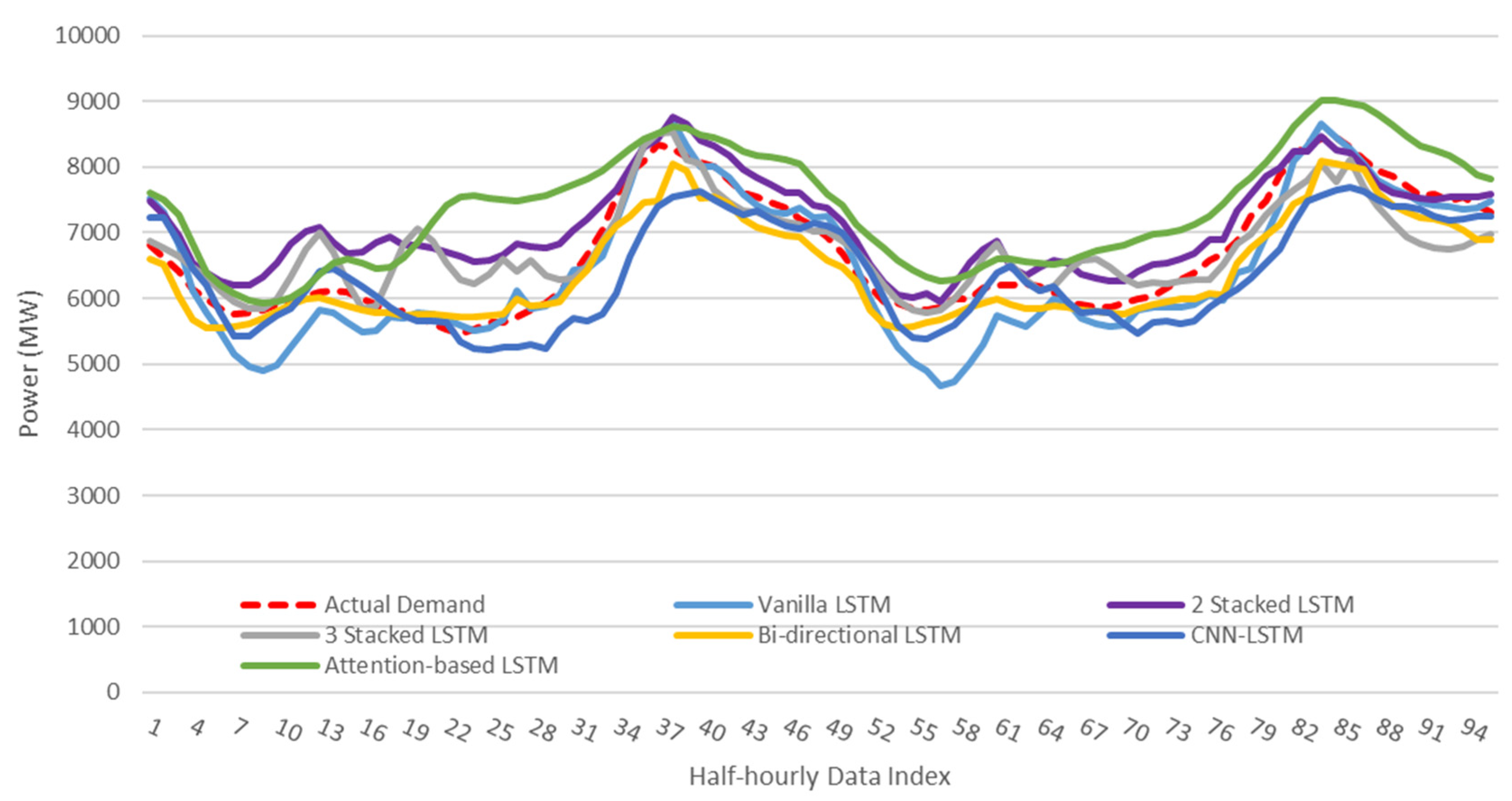
The evaluation focuses on the last day of the year, with 24 timeslots, but for better visualization, 48 h is illustrated using half-hourly indices. Figure 6 compares the demand forecasted by various LSTM networks with the actual demand. Although most models follow the overall pattern of the actual data, they fail to capture the fluctuations effectively, especially during low-demand periods. Specifically, the CNN-LSTM model tends to underestimate the load demand, while the attention-based model overestimates it. The Bi-directional LSTM appears to perform better in capturing load variations. To quantify the performance of the LSTM models,

Table 3. Values of metrics for predicted demand.

Method	MAE	MSE	RMSE	R2 Score	MAPE
Vanilla LSTM	301.525	133,265.213	365.055	0.8435	4.365
2-Stacked LSTMs	386.506	216,900.633	465.726	0.745	5.796
3-Stacked LSTMs	294.259	138,272.484	371.850	0.837	4.335
Bi-dir LSTM	439.369	616,884.953	785.420	0.275	6.160
CNN-LSTM	396.339	268,141.446	517.823	0.6851	5.556
Att-based LSTM	490.747	379,234.346	615.820	0.554	6.978

presents various metrics. While each metric may rank the models differently, the Vanilla LSTM and 3-Stacked LSTM generally demonstrate superior performance in load demand forecasting.

As previously mentioned, the same data resolution is used for price forecasting. However, the actual price values exhibit greater volatility, making accurate prediction more challenging. Price is the second dependent variable in the models, leading to difficulties in capturing peaks and valleys, and models often only follow the overall price trend. Figure 7 shows that the 3-Stacked LSTM performs better than other models. It is important to note that this figure represents only 96 data points out of the total 17,520 samples.

Table 4. Values of metrics for predicted price.

Method	MAE	MSE	RMSE	R2 Score
Vanilla LSTM	13.904	333.572	18.263	0.227
2-Stacked LSTMs	13.326	303.278	17.414	0.297
3-Stacked LSTMs	12.813	301.489	17.363	0.3015
Bi-dir LSTM	13.986	366.799	19.152	0.1502
CNN-LSTM	15.648	399.537	19.988	0.074
Att-based LSTM	14.542	356.522	18.881	0.174

quantifies the accuracy of each model using metrics formulated in Section 3.4. According to these metrics, the 3-Stacked LSTM consistently outperforms other models in price forecasting, followed by the 2-stacked and Vanilla LSTM architectures.

Table 5. GPU resource usage.

Method	Number of Epochs (Optimized)	GPU Memory (GB)	Average Time per Epoch (s)
Vanilla LSTM	47	0.3	2
2-Stacked LSTMs	42	0.3	2
3-Stacked LSTMs	46	0.3	3
Bi-dir LSTM	21	0.3	2
CNN-LSTM	64	0.3	2
Att-based LSTM	54	0.3	2

presents the resource usage of the various LSTM configurations examined. Among them, the CNN-LSTM model requires more epochs to reach optimization. However, since the duration of each epoch varies, the table includes the average time per epoch, reflecting the time most epochs take. Despite the differences in model configurations, the GPU memory usage remains constant across all models due to the dataset’s volume.

Figure 8 illustrates the impact of forecasted demand and price values on the deviation of optimal operational costs across various proposed architectures. Despite the higher accuracy in forecasting shown by the 3-stacked LSTM and Vanilla LSTM models, they led to larger deviations in the optimal values of the energy management problem. Conversely, the attention-based LSTM demonstrated less deviation from the actual optimal operational cost of the microgrid. As depicted, the range of deviation from optimal values spans from a minimum of 25% to a maximum of 40%.

5. Conclusions

This paper presents and compares multivariate Long Short-Term Memory (LSTM) approaches for microgrid energy management systems, focusing on the correlation between electricity load demand and price in the neural networks used for the forecasting module. Our findings highlight that incorporating the complexity of correlation between two dependent variables may reduce accuracy compared to univariate predictions, where only one dependent variable is present in the model’s response set. Unlike univariate models, where the prediction focuses on a single variable, multivariate models must account for the interactions and dependencies between multiple variables. These interactions can introduce additional noise and complexity into the model, making it harder to achieve the same level of accuracy as with univariate models, where the focus is more straightforward. However, it is important to note that while the initial accuracy might appear reduced, the multivariate approach provides a more holistic and realistic representation of the system, capturing the intricate relationships between variables that are crucial for informed decision-making in energy management systems. Despite this, multivariate forecasting offers the advantage of capturing the interplay between demand and price data, although it may lead to less accurate output due to the increased model complexity. In scenarios where a single model is required to predict two dependent variables in an energy management system, our results show that a stacked LSTM with three layers performs better in predicting both demand and price, followed closely by the Vanilla LSTM. These results underscore that higher accuracy in machine learning models does not necessarily translate to more optimal or minimal cost outcomes for energy management. The observed deviation of up to 40% from the optimal operational cost highlights the need to scrutinize forecasted values thoroughly before decision-making. Future research can enhance these models by incorporating correlation measures or coefficients between variables as additional features, aiding the model in better capturing the relationships. Additionally, implementing an attention mechanism to assign importance to different variables at various time steps, especially during peak load demand periods, presents a promising direction for future investigation. This approach could improve the model’s focus on relevant information and potentially enhance prediction performance.