Quantifying Uncertainty with Conformal Prediction for Heating and Cooling Load Forecasting in Building Performance Simulation

Abstract

Building Performance Simulation extensively uses statistical learning techniques for quicker insights and improved accessibility. These techniques help understand the relationship between input variables and the desired outputs, and they can predict unknown observations. Prediction becomes more informative with uncertainty quantification, which involves computing prediction intervals. Conformal prediction has emerged over the past 25 years as a flexible and rigorous method for estimating uncertainty. This approach can be applied to any pre-trained model, creating statistically rigorous uncertainty sets or intervals for model predictions. This study uses data from simulated buildings to demonstrate the powerful applications of conformal prediction in Building Performance Simulation (BPS) and, consequently, to the broader energy sector. Results show that conformal prediction can be applied when any assumptions about input and output variables are made, enhancing understanding and facilitating informed decision-making in energy system design and operation.

1. Introduction

Integrated energy systems consist of different components that interact through various energy pathways. Understanding how these systems perform under changing conditions, where user demand and energy prices fluctuate, requires a simulation tool [1].

Building Performance Simulation (BPS) [2] shows the potential to provide valuable design insights by suggesting design solutions. These tools are extensively utilized across various fields because they allow experimentation with parameters otherwise impractical or challenging to control in real-world settings. Employing sophisticated, specialized building energy simulation software can offer valuable solutions for estimating the effects of various building design options. Nonetheless, this approach can be highly time-intensive and demands expertise from users in a specific program. Furthermore, simulation tools face challenges due to the complexity of parameters and factors like nonlinearity, strong interactions, and uncertainty.

Hence, in practical applications, numerous researchers employ statistical learning methods to evaluate the influence of different building parameters (such as compactness) on specific variables of interest (such as energy consumption). A possible example can be found in Tsanas et al. (2012) [3]. This approach is frequently preferred due to its reduced computational burden and increased accessibility, mainly when a database is accessible. By harnessing statistical learning principles, advanced methods can be utilized to analyze and explore the energy efficiency of buildings, enabling swift comprehension of the impacts of diverse building design parameters once the model is appropriately trained. To this end, statistical analysis can enrich comprehension by gauging the relationship between input variables (i.e., covariates, predictors, or input) and the desired output (i.e., target, response variable, or outcome), identifying the most influencing variables [4]. The incorporation of statistical learning in energy performance analysis has generated substantial interest.

In supervised statistical learning applications, the goal is to make point predictions that closely approximate the actual values of continuous processes. Point predictions are singular values that best estimate a future output based on historical data. They are commonly used in scenarios where the objective is to predict a continuous variable, such as the heating and cooling loads. While point predictions are valuable, prediction can be more informative if represented by probability distributions. In this approach, the quantification of uncertainty [5,6,7] allows for more informed energy analysis.

Uncertainty assessment has gained increasing significance in the context of building energy analysis. Uncertainty analysis in BPS is more related to estimating the impact of input variables on the output considered. For example, Tiana et al. (2018) [8] presented different approaches and applications for controlling and understanding the uncertainty coming from input variables. This is primarily due to the unpredictability of key factors that impact building performance, such as occupant behavior and the thermal characteristics of building envelopes. Uncertainty analysis has been widely utilized in various domains of building energy analysis, encompassing model calibration, life cycle assessment, analysis of building stock, evaluation of climate change impact and adaptation, sensitivity analysis, spatial analysis, and optimization.

As mentioned, uncertainty is connected with the estimation of statistical prediction intervals. Different techniques are available in the literature for building prediction intervals as reviewed by Tian et al. (2022) [9]. As confidence intervals are used to quantify uncertainty about parameters and functions of parameters, prediction intervals offer a natural method for quantifying prediction uncertainty. Traditional prediction intervals have limitations regarding distributional or model assumptions that limit their use in real applications.

Over the past 25 years, a new method for prediction interval quantification, the so-called conformal prediction (CP), has been introduced and developed. In their study, Vovk and colleagues (2009) [10] introduced a sequential method for constructing prediction intervals, forming the foundation for developing the conformal prediction framework. Conformal prediction (CP), also referred to as conformal inference, represents a user-friendly paradigm for establishing statistically robust uncertainty sets or intervals for model predictions. Essentially, CP utilizes prior knowledge to develop accurate confidence levels in new predictions. This approach is versatile, as it can be implemented with any pre-trained model, including neural networks or random forests, to produce prediction sets that are guaranteed to contain the actual value with a specific probability, such as 90%.

The main contribution of this work is to leverage data from simulated buildings to demonstrate the robust potential of conformal prediction in Building Performance Simulation (BPS) and its broader implications for the energy sector. To achieve this, data from 768 simulated buildings will be utilized [3]. Initially, we will develop a heating and cooling load prediction model using the available input variables. Following that, we will build prediction intervals for the target variables based on the split conformal prediction method as described in the work by Lei et al. (2018) [11]. The results indicate that conformal prediction can be effectively applied across various input and output variable assumptions, thereby improving understanding and facilitating well-informed decision-making in the design and operation of energy systems.

This paper is organized as follows. Section Related Literature presents the related literature. Section 2 introduces the methodological framework and theory underlying conformal prediction. In Section 3, we present the simulation study. First, we compare different statistical learning models, and then we focus our analysis on hyper-parameter tuning for random forests. Section 4 discusses the primary advancements in conformal prediction, and Section 5 concludes the work.

Related Literature

In practical applications, high accuracy in predicting continuous variables, such as cooling or heating demands, is often the main objective. Point prediction is surely really important; however, the estimation of predictive uncertainty permits more informed decision-making under conditions of uncertainty.

In statistics, predictive uncertainty can be computed mainly with two approaches: (i) identifying the frequentist prediction intervals [12] and (ii) estimating the posterior predictive distribution for Y (i.e., target or output variable) in the Bayesian framework [13].

For Building Performance Simulation (BPS), many efforts have been made to quantify predictive uncertainty in the output variable. In the work of Zhang et al. (2020) [14], the authors proposed a generic prediction interval estimation method for the uncertainty estimation of predicted cooling loads based on quantile estimation. A dataset of real building consumption based on China, more precisely, Shenzhen, is used to test the proposed approach. Similarly, Dong et al. (2022) [15] proposed an interval prediction method based on kernel density estimation for cooling loads. In this study, the data were collected by the University of Texas, Austin. In the context of structural design simulation models, Shabbir et al. (2024) [16] proposed the use of Artificial Neural Networks (ANNs) to estimate prediction intervals for evaluating the seismic performance of buildings exposed to long-term ground motion.

An example of using the Bayesian framework can be found in the work of Braulio-Gonzalo et al. (2016) [17]. In this work, the authors use Bayesian inference for the prediction of building energy performance by exploiting EnergyPlus (US Department of Energy. EnergyPlus https://energyplus.net/ (accessed on 26 August 2024)) software (version 8.10). EnergyPlus is used in combination with the Design Builder interface. The software computes the response variables—namely, energy demand for heating and cooling, as well as discomfort hours for both heating and cooling. These calculations are performed for a set of simulated buildings characterized by a combination of input variables, including year of construction, building shape factor, solar orientation, street height–width ratio, and urban block type. The results from these simulations are then used as input data to develop the prediction models. An interesting area of research based on Bayesian inference, and consequently on Bayesian predictive distribution, can be found on building energy performance calibration [18].

Inspired by the work of LeRoy et al. (2021) [19], in this work, we propose for the first time the use of conformal inference for uncertainty estimation of the predicted target variables under consideration in BPS.

2. Conformal Prediction

In this section, following the work of Lei et al. (2018) [11], we briefly introduce the methodological aspect of conformal prediction for regression.

Given independent and identically distributed (i.i.d.) regression data $Z_i={(X_i,Y_i)}_{i=1}^n$ drawn from a distribution P, where each $Z_i$ consists of an outcome $Y_i$ and a d-dimensional input vector $X_i=(X_i\left(1\right),\dots ,X_i\left(d\right))$, we aim to predict the outcome $Y_{n+1}$ for a new input vector $X_{n+1}$. For an example of regression processing from an application point of view, please see [20].

The final aim is to build a prediction interval $C\subset {\mathbb{R}}^d\times \mathbb{R}$, that is:

$$P(Y_{n+1}\in C\left(X_{n+1}\right))\ge 1-\alpha ,$$

(1)

where $\alpha$ is a specified miscoverage level. The probability $P(Y_{n+1}\in C\left(X_{n+1}\right))$ is computed on $n+1$ i.i.d. draws $Z_1,\dots ,Z_n,Z_{n+1}\sim P$. For an observation $x\in {\mathbb{R}}^d$, $C\left(x\right)$ represents the set of possible responses $y\in \mathbb{R}$ such that $(x,y)\in C$. The prediction band should have finite-sample (nonasymptotic) validity without assumptions on P.

A possible simple approach for building a prediction interval for $Y_{n+1}$ could be the following one. Now, we consider $Y_{n+1}$ at the new outcome $X_{n+1}$, with $(X_{n+1},Y_{n+1})$ being an independent sample taken from P. Given the previous description, a possible way to build a prediction interval is:

$$C_{\mathrm{naive}}\left(X_{n+1}\right)=\left[\widehat{\mu }\left(X_{n+1}\right)-{\widehat{F}}_n^{-1}(1-\alpha ),\widehat{\mu }\left(X_{n+1}\right)+{\widehat{F}}_n^{-1}(1-\alpha )\right],$$

(2)

where $\widehat{\mu }$ is the regression function estimator, and ${\widehat{F}}_n$ is the empirical distribution of the difference between observed outcome values and predicted one (i.e., fitted residuals) $|Y_i-\widehat{\mu }\left(X_i\right)|$ for $i=1,\dots ,n$. The term ${\widehat{F}}_n^{-1}(1-\alpha )$ represents the $(1-\alpha )$-quantile of ${\widehat{F}}_n$. In the case of a great sample, the interval is approximately valid if $\widehat{\mu }$ is reliable. Specifically, this means that the estimated $(1-\alpha )$-quantile ${\widehat{F}}_n^{-1}(1-\alpha )$ of the fitted residual distribution should be close to the $(1-\alpha )$-quantile of the population residuals $|Y_i-\mu \left(X_i\right)|$ for $i=1,\dots ,n$. Guaranteeing this level of precision for $\widehat{\mu }$ typically necessitates proper regularity conditions on the underlying data distribution P and on $\widehat{\mu }$ itself. These conditions include having a correctly specified model and selecting appropriate tuning parameters.

Generally, the naive approach (Equation (2)) may significantly underestimate uncertainty due to potential biases in the fitted residual distribution. Conformal prediction intervals address these limitations of naive intervals. Remarkably, they ensure proper finite-sample coverage without making any assumptions about P or $\widehat{\mu }$, except that $\widehat{\mu }$ behaves as a symmetric function of the data points.

We now use an alternative approach. For each $y\in \mathbb{R}$, we develop an estimator of the regression function ${\widehat{\mu }}_y$, based on an enlarged (i.e., augmented) set of data $Z_1,\dots ,Z_n,(X_{n+1},y)$. Next, specify

$$R_{y,i}=|Y_i-{\widehat{\mu }}_y\left(X_i\right)|\mathrm{for}i=1,\dots ,n,\mathrm{and}{R}_{y,n+1}=|y-{\widehat{\mu }}_y\left(X_{n+1}\right)|,$$

(3)

and order $R_{y,n+1}$ among the remaining fitted residuals $R_{y,1},\dots ,R_{y,n}$. Then, compute

$$\pi \left(y\right)={\displaystyle \frac{1}{n+1}}\sum _{i=1}^{n+1}1\{R_{y,i}\le R_{y,n+1}\}={\displaystyle \frac{1}{n+1}}+{\displaystyle \frac{1}{n+1}}\sum _{i=1}^{n}1\{R_{y,i}\le R_{y,n+1}\},$$

(4)

the fraction of points in the augmented sample with a fitted residual less than the last, $R_{y,n+1}$. $1\{·\}$ denotes the indicator function.

Given the data exchangeability and the symmetry of $\widehat{\mu }$ on $y=Y_{n+1}$, the constructed statistic $\pi \left(Y_{n+1}\right)$ is uniformly distributed over the set $\{1/(n+1),2/(n+1),\dots ,1\}$. This indicates

$$P\left((n+1)\pi \left(Y_{n+1}\right)\le \lceil (1-\alpha )(n+1)\rceil \right)\ge 1-\alpha ,$$

(5)

implying that $1-\pi \left(Y_{n+1}\right)$ is a suitable (conservative) p-value for the hypothesis test condition $H_0:Y_{n+1}=y$.

By reversing the test for all $y\in \mathbb{R}$, we obtain the conformal prediction interval at $X_{n+1}$:

$$C_{\mathrm{conf}}\left(X_{n+1}\right)=\left\{y\in \mathbb{R}:(n+1)\pi \left(y\right)\le \lceil (1-\alpha )(n+1)\rceil \right\}.$$

(6)

The process must be repeated for every prediction interval at a new input value. In practice, we limit the consideration in Equation (2) to a discrete set of trial values y.

When constructed in this way, the conformal prediction band in Equation (2) guarantees valid finite-sample coverage and accuracy, preventing significant over-coverage.

As previously discussed, the original conformal prediction method demands significant computational resources. For any $X_{n+1}$ and y, determining whether y belongs to $C_{\mathrm{conf}}\left(X_{n+1}\right)$ requires training the model again on the new enlarged dataset that contains the new observation $(X_{n+1},y)$, and to calculate and order once again the absolute residuals.

An alternative approach, the so-called split conformal prediction, is also available in the literature. This method is entirely general, with only a fraction of the computational cost of the full conformal method. This method segments the two phases of the previous procedure, more precisely, fitting and ranking, by considering sample splitting by creating an inference set and a learning or calibration set. This split leads to a computational cost equal to the fitting time of the chosen model.

Its principal coverage properties are as follows: if $(X_i,Y_i),i=1,\dots ,n$ are independent and identically distributed, then for a new i.i.d. observation $(X_{n+1},Y_{n+1})$,

$$P\left(Y_{n+1}\in C_{\mathrm{split}}\left(X_{n+1}\right)\right)\ge 1-\alpha ,$$

(7)

where $C_{\mathrm{split}}$ is the split conformal prediction interval build based on Algorithm 1 [11]. Furthermore, if we also assume that the residuals $R_i,i\in I_2$, where $I_2$ is the calibration set, have a continuous joint distribution, then

$$P\left(Y_{n+1}\in C_{\mathrm{split}}\left(X_{n+1}\right)\right)\le 1-\alpha +{\displaystyle \frac{2}{n+2}}.$$

(8)

Aside from its substantial computational efficiency relative to the initially described method, the presented modification can also offer advantages regarding memory requirements. See Lei et al. (2018) [11] for more details.

Algorithm 1 Split conformal prediction.

Input: Dataset $(X_i,Y_i)$, $i=1,\dots ,n$ Supervised learning model $\widehat{\mu }$ Miscoverage level $\alpha \in (0,1)$ Output: Prediction band, over $x\in {\mathbb{R}}^d$ Step 1: Randomly split $\{1,\dots ,n\}$ into equal-sized subsets $I_1$, $I_2$ Step 2: Train ${\widehat{\mu }}_{I_1}=\mu \left(\{(X_i,Y_i):i\in I_1\}\right)$ Step 3: Compute the score function (e.g., residuals) $R_i=|Y_i-{\widehat{\mu }}_{I_1}\left(X_i\right)|:i\in I_2$ Step 4: Sort $\{R_i:i\in I_2\}$ in increasing order $R_{\left(1\right)}\le \cdots \le R_{(n/2)}$ Step 5: Compute $d=R_{\left(k\right)}$ that is the k-th smallest value in $\{R_i:i\in I_2\}$, where $k=\lceil (1-\alpha )(n/2+1)\rceil$ Return: $C_{\mathrm{split}}\left(x\right)=[{\widehat{\mu }}_{I_1}\left(x\right)-d,{\widehat{\mu }}_{I_1}\left(x\right)+d]$, for all $x\in {\mathbb{R}}^d$

3. Prediction Intervals for Building Performance Simulation

In this work, we exploit the data presented by Tsanas et al. (2012) [3] (Data are available at https://archive.ics.uci.edu/dataset/242/energy+efficiency (accessed on 26 August 2024)). To summarize, they generated 12 different buildings using simple combinations of elements (i.e., cubes), resulting in 720 building samples with varying surface areas and dimensions. All buildings have the same volume (771.75 m³) but differ in other characteristics. The building materials chosen for their common use and low U-values consist of walls, floors, roofs, and windows. The simulations assume residential conditions in Athens, Greece, with seven occupants engaging in sedentary activities (70W). Internal design conditions include specific clothing (0.6 clo), humidity (60%), airspeed (0.30 m/s), and lighting level (300 Lux). Internal gains are set at sensible (5) and latent (2 W/m²), with an infiltration rate of 0.5 air changes per hour and a wind sensitivity of 0.25. Thermal properties are configured with 95% efficiency, a thermostat range of 19 °C to 24 °C, and operational hours of 15–20 on weekdays and 10–20 on weekends. The buildings feature three types of glazing areas (10%, 25%, and 40% of floor area) distributed across five scenarios (uniform, north, east, south, and west) for each glazing type. Additionally, samples without glazing are included. All building forms are simulated in four orientations (facing the four cardinal points), resulting in 768 unique building configurations (720 with glazing variations and 48 without).

For each building, the following data about relative compactness ($X_1$), surface area ($X_2$), wall area ($X_3$), roof area ($X_4$), overall height ($X_5$), orientation ($X_6$), glazing area ($X_7$), and glazing area distribution ($X_8$) are gathered. Furthermore, the heating load (HL) and cooling load (CL) are stored and considered target variables. Respectively, $Y_1$ and $Y_2$. Figure 1 shows the distribution of HL and CL.

In this work, we first compare statistical learning models for predicting HL and CL target variables and compute split conformal prediction intervals for uncertainty estimation. The comparison is made using Mean Squared Error (MSE), empirical coverage, and the length of the prediction interval. Empirical coverage is the average number of times the actual value of the target variable falls within the conformal prediction interval. The length of the prediction interval is the difference between the upper and lower conformal bounds.

Next, we demonstrate tuning a specific statistical learning model based on prediction accuracy and split conformal prediction intervals. This latter experimental simulation is also used to empirically verify that conformal inference guarantees reliable coverage under the assumption of independent and identically distributed (i.i.d.) data.

The experiments are executed on an Intel Core i5-1035G4 CPU with a base clock speed of 1.10 GHz, 4 cores, and 8 threads. The code is written in R language programming [21] (R version 4.3.2), and the conformalInference [22] (version 1.1), randomForest [23] (version 4.7-1.1), neuralnet [24] (version 1.44.2), and e1071 [25] (version 1.7-14) packages are used (All codes are available at https://github.com/matteoborrotti/conforma-prediction-for-Building-Performance-Simulation.git (accessed on 26 August 2024)).

3.1. Comparison of Statistical Learning Models

Predicting energy consumption is a crucial task in performance monitoring, and accurate predictions are essential for Building Performance Simulation (BPS). The literature provides various comparative analyses of statistical and machine learning techniques for BPS. For example, Chakraborty et al. (2018) [26] present a comprehensive overview of the workflow for applying statistical learning techniques in BPS, detailing the intermediate procedures for feature engineering, feature selection, and hyper-parameter optimization.

Similarly, in this work, we compare different approaches for predicting heating load (HL) and cooling load (CL) target variables. We also analyze these approaches using split conformal prediction intervals. Specifically, we apply forward stepwise regression (stepwise), support vector machine (SVM) [27], random forest (RF) [28], and neural network (NN) [29]. Forward stepwise regression and random forest are included in the conformalInference package. For SVM, and NN, we create ad hoc functions to integrate these statistical learning techniques into the conformalInference package.

All techniques are used with the default settings of the respective R packages. For clarity, forward stepwise regression is used with a maximum of 20 steps for variable selection. The SVM kernel is set to linear. The number of trees grown in the random forest (RF) is set to 500, with 2 variables randomly sampled at each split in constructing the decision trees (m). The NN architecture is a feed-forward NN with one hidden layer and 8 nodes. For all other parameters, please refer to the original R packages.

The results are summarized in

Table 1. Average values for test MSE, empirical average coverage, and average length for heating ($Y_1$) target variable results are averages over 50 repetitions. Standard deviations are reported in parentheses.

Models	Test MSE	Empirical Coverage	Length of Intervals
Neural Net	0.48 (0.23)	0.90 (0.02)	2.09 (0.53)
Random Forest	1.75 (0.19)	0.91 (0.01)	4.07 (0.87)
Stepwise	8.58 (0.19)	0.91 (0.02)	11.83 (0.45)
SVM	8.54 (0.15)	0.92 (0.02)	12.33 (0.87)

and

Table 2. Average values for test MSE, empirical average coverage, and average length for heating ($Y_2$) target variable results over 50 repetitions. Standard deviations are reported in parentheses.

Models	Test MSE	Empirical Coverage	Length of Intervals
Neural Net	3.04 (0.63)	0.92 (0.02)	6.84 (0.69)
Random Forest	3.41 (0.20)	0.91 (0.01)	6.85 (0.42)
Stepwise	10.80 (0.24)	0.88 (0.02)	10.88 (1.15)
SVM	10.71 (0.16)	0.89 (0.01)	10.52 (1.08)

. Average values for test Mean Squared Error (MSE), empirical average coverage, and average length of conformal intervals are reported. All results are averaged over 50 repetitions, with standard deviations provided in parentheses.

Table 1 presents the values for the target variable $Y_1$. Forward stepwise regression and SVM perform similarly, likely due to using a linear kernel for SVM, which fails to capture the nonlinear nature of the phenomenon. The two best models are RF and NN, with NN outperforming all other models. In this case, coverage is ensured by all the methods used. The average interval length indicates that forward stepwise regression and SVM are more uncertain in predicting the target variable $Y_1$. In contrast, the predictions of RF and NN are more accurate.

All models are less reliable regarding the predictions of the target variable $Y_2$ (see Table 2). Forward stepwise regression and SVM are confirmed as the two methods with the worst results across all considered metrics. The behavior of RF and NN differs from the previous case. While NN is the best method for predicting $Y_1$, for $Y_2$, the two methods are equivalent. RF proves to be slightly more stable, presenting a lower standard deviation than NN.

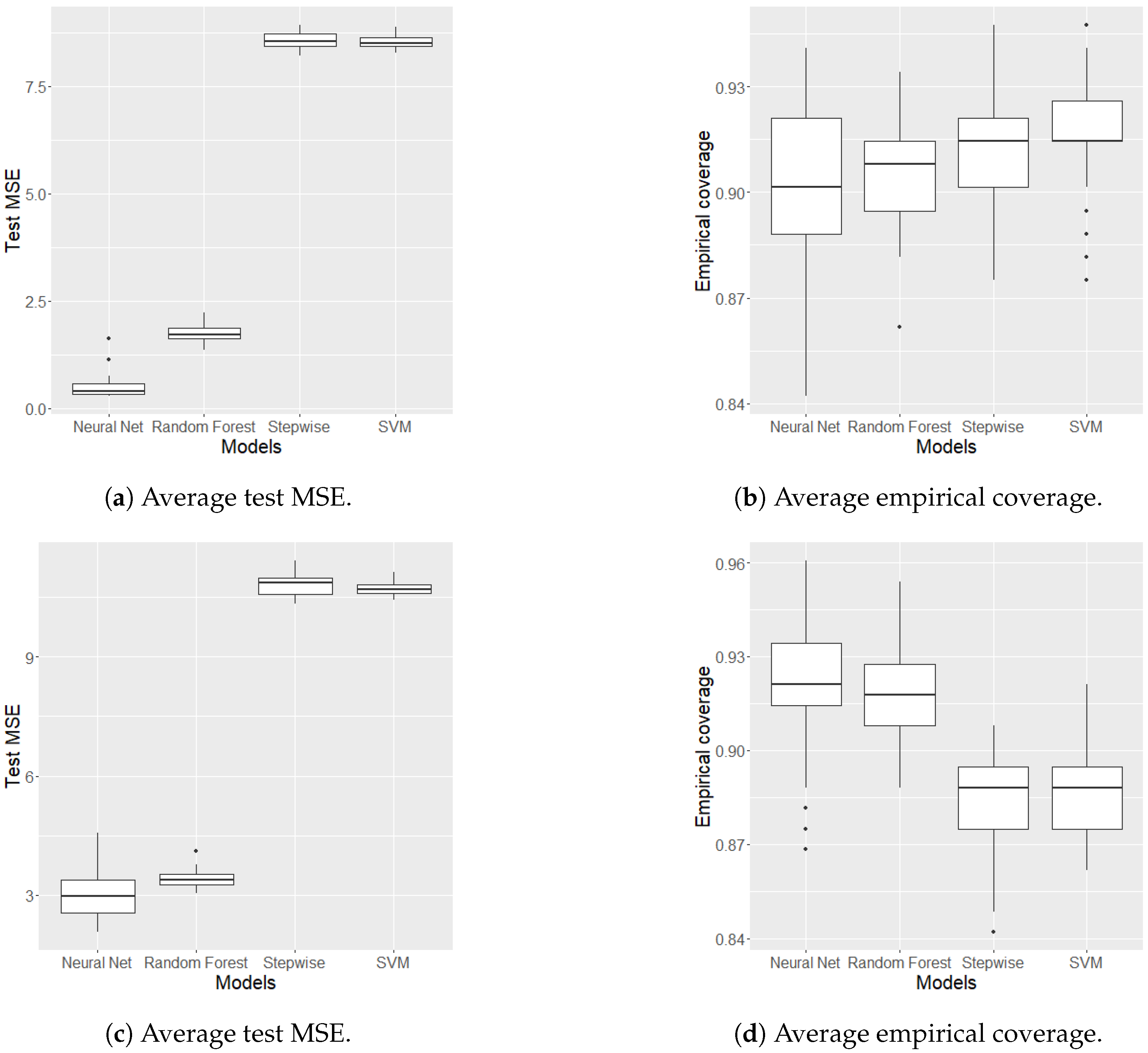
Figure 2 shows the distributions of the MSE test values and empirical coverage over 50 repetitions using boxplots. Figure 2a,b show the performance of the methods on the target variable $Y_1$, while Figure 2c,d show the performance on the target variable $Y_2$. The previous observations made from the results in Table 1 and Table 2 are confirmed here. Forward stepwise regression and SVM fail to capture the nonlinear relationship between target and input variables, resulting in the worst performance. NN and RF are the two best methods, with NN proving to be the best for predicting $Y_1$. For $Y_2$, the two methods are equivalent, though NN is slightly better. However, RF is more stable due to the low variability of the boxplots in terms of MSE test values.

Given these considerations—the equivalence of the two methods in the more challenging task of predicting $Y_2$ and the greater stability of RF—we are confident that optimizing the RF hyper-parameters will yield better results.

3.2. Hyper-Parameter Optimization

Conformal prediction offers reliable coverage under no assumptions other than i.i.d data. We now empirically study this property and the behavior of the conformal prediction interval by optimizing the hyper-parameter m of the random forest model [28]. The hyper-parameter m controls the number of variables randomly sampled at each split in constructing the decision trees. m ranges between 2 and 8, where $m=8$ corresponds to a Bagging model [30]. Conformal prediction intervals are computed and analyzed for heating ($Y_1$) and cooling load ($Y_2$) variables. All results are averages over 50 repetitions. Additionally, all intervals are computed at the 90% nominal coverage level using a split conformal prediction that is valid under no assumptions.

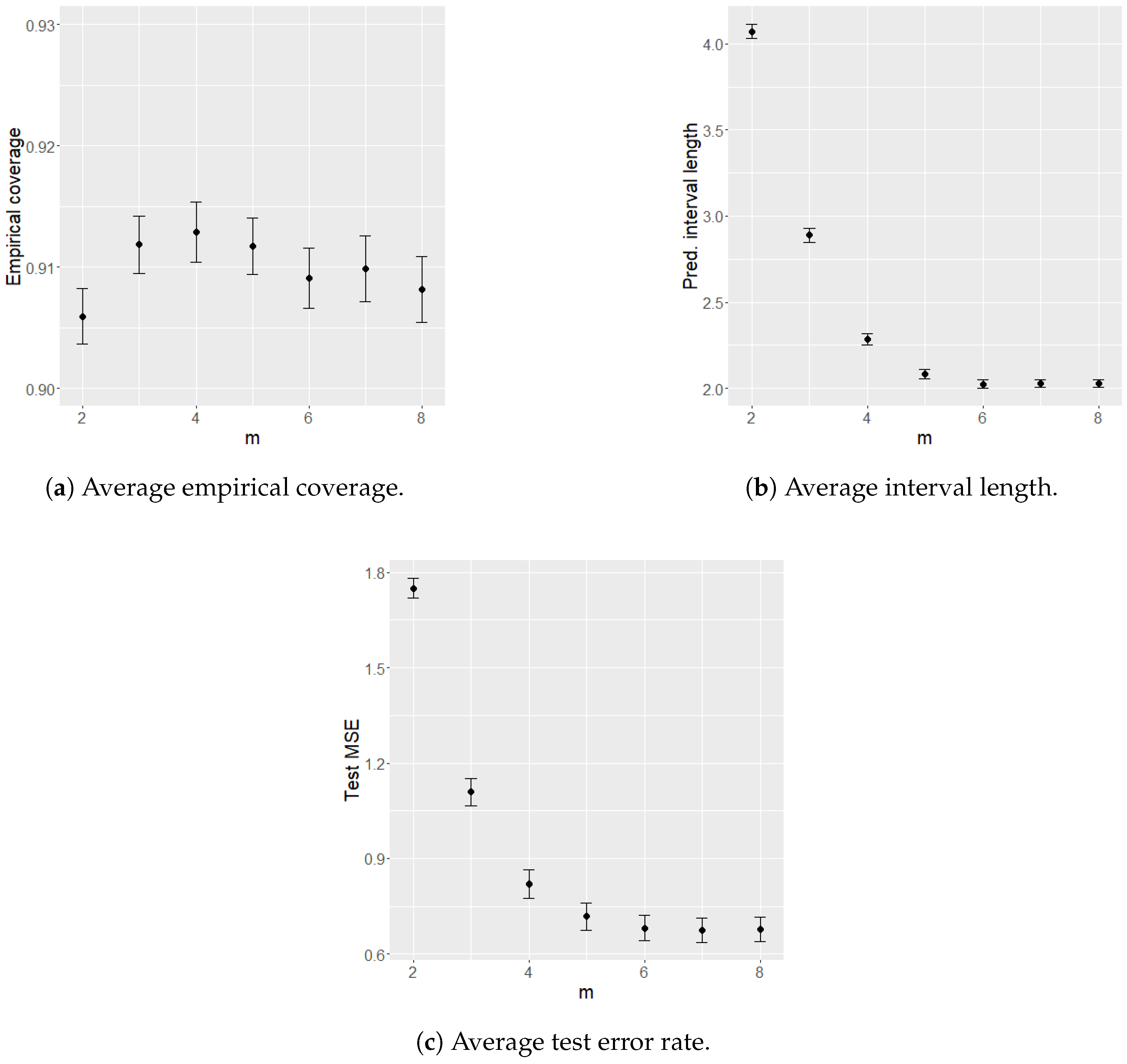
In both cases (Figure 3 and Figure 4), it is observed that across all settings, regardless of test error performance, the coverage of the conformal intervals consistently approximates the nominal level of 90%. Additionally, the interval lengths vary concerning the target variables, demonstrating a strong correlation with test errors [11].

For the target variable $Y_1$ (Figure 3), the test error is minimal across all settings, corresponding to tiny prediction interval lengths. This suggests that the model effectively captures the relationship between the response and input variables. On the contrary, for the target variable $Y_2$ (Figure 4), the test errors are significantly higher for each value of m. This increased error is reflected in broader prediction intervals, indicating a lower accuracy of the random forest method in predicting the cooling load target variable ($Y_2$). Furthermore, in Figure 3c, the average MSE test exhibits a particular behavior. As the number of variables randomly sampled at each split increases, the MSE test initially decreases, reaching a minimum point, then increasing again, leading to worse results. When the lowest MSE test value is reached, using more variables for the split definition can cause overfitting of the training set, thereby reducing the model’s generalization ability. Generalizing ability refers to the model’s capability to accurately predict new observations not used during the training phase. More precisely, increasing the number of variables randomly sampled at each split (m) in the RF can reduce bias but increase the risk of overfitting the training set due to higher variance.

4. Discussion

Conformal prediction intervals provide distribution-free coverage guarantees. However, as illustrated in Section 3, conformal inference can be utilized to evaluate the reliability of regression methods. The prediction intervals meet the required coverage conditions if the model is correctly specified for the data under study. Conversely, if the model is misspecified, the intervals remain valid but may only ensure marginal coverage. Given these considerations, conformal prediction intervals effectively compare statistical learning models.

Conformal prediction ensures predictive coverage when the data points $(X_i,Y_i)$ are drawn independently and identically distributed (i.i.d.) from any distribution. However, the validity of this method depends on the assumption that the data points are drawn independently from the same distribution or, more broadly, that $(X_1,Y_1),\dots ,(X_{n+1},Y_{n+1})$ are exchangeable. This assumption is often violated in practical applications due to distribution drift, correlations between data points, or other phenomena. Barber et al. (2023) [31] introduced weighted quantiles to enhance robustness against distribution drift and developed a new randomization technique to accommodate algorithms that do not treat data points symmetrically. This advancement extends the applicability of conformal prediction to a wide range of energy applications. For instance, Barber et al. (2023) [31] demonstrated the applicability of the proposed methods using a dataset comprising electricity consumption and pricing information from the regions of New South Wales and Victoria, Australia. The dataset spans 2.5 years, from 1996 to 1999, with data recorded at 30 min intervals. The potential applications of the solutions proposed by Barber et al. (2023) [31] extend to the domain of renewable energy, which presents significant challenges for power integration systems. Accurate predictions of renewable energy output and calibrated uncertainty estimates provide financial benefits to electricity suppliers and are crucial for grid operators to optimize operations and prevent grid imbalances.

In this study, we focus on a regression problem. Conformal inference also applies to binary and multi-class classification problems [32]. In these cases, a prediction interval can be interpreted as the set of possible classes most likely to include the true class of the new observation. A possible application is the classification of different energy usage patterns, including in residential, commercial, and industrial settings, allowing for customizing energy supply strategies and improving the accuracy of predicting energy demand. Utilizing conformal inference helps quantify the confidence in these classifications, ultimately enhancing the reliability of demand forecasts and optimizing resource allocation in the energy grid. Another field of application is related to power system reliability, where accurately diagnosing the type of fault—such as short circuit, grounding fault, or line-to-line fault—is essential for enabling prompt and precise maintenance actions. By leveraging conformal inference for multi-class classification, the uncertainty in fault diagnosis can be quantified, leading to more reliable decision-making and minimizing downtime in the electrical grid.

Conformal prediction represents an exciting new area of research. Various reviews [32,33,34] available in the literature enable researchers and practitioners to explore and engage with this field. Shafer et al. (2008) [33] provided a complete technical review of conformal prediction ranging from the basic theoretical aspects (Fisher’s prediction interval) to more advanced topics, such as exchangeability. A set of examples are provided for demonstrating the theoretical aspects previously introduced. The work of Angelopoulos et al. (2021) [32] is a practical introduction that comprehensively explains conformal prediction. This work provides both practical theory and real-world examples. It also covers new improvements related to a set of challenging statistical learning tasks, such as distribution shift, time-series analysis, and outliers detection. Fontana et al. (2023) [34] presented the conformal inference framework from a different perspective, investigating the concept of statistical validity and analyzing the computational problems arising from conformal prediction. All together, these reviewers can give a complete understanding of conformal inference and, additionally, provide an important source of literature as a place to start for further investigation.

5. Conclusions

Conformal prediction is a user-friendly approach that generates statistically rigorous uncertainty sets or intervals for model predictions. Additionally, it guarantees predictive coverage when the data points $(X_i,Y_i)$ are independently and identically distributed (i.i.d.) from any distribution.

This work uses data from 768 unique simulated buildings to demonstrate the effectiveness of conformal prediction. Eight input variables and two responses are considered. Two random forests are trained to predict both the response variables. Conformal prediction is used to compute prediction intervals with any assumptions on the distributions of the variables. All intervals are calculated at the 90% nominal coverage level using a split conformal prediction technique. Initially, we evaluate various statistical learning models—specifically, forward stepwise regression, support vector machines, random forests, and neural networks—by assessing their predictive performance through conformal prediction intervals. Subsequently, we concentrate on random forests, with a detailed examination of the hyper-parameter m to enhance predictive accuracy. Across all considered hyper-parameter settings of random forests, it is observed that the coverage of the conformal intervals consistently approximates the nominal level of 90%, regardless of test error performance. Furthermore, the interval lengths vary according to the two target variables, showing a strong correlation with test errors.

Considering uncertainties could improve and enable design decision support, particularly if it were to be augmented by techniques for variable interpretation. Lei et al. (2018) [11] proposed the leave-one-covariate-out (LOCO) inference, a model-free notion of variable importance. LOCO can be used to estimate the importance of each variable in a prediction model, enabling better interpretation of the results and impact of each variable on the simulation.

In future work, LOCO techniques could assess variable importance when treating the working model as incorrect. Moreover, Section 4 discusses the limitations of the conformal prediction technique used in this work. The main assumption of conformal prediction is that the data are exchangeable. This assumption is often violated. To overcome this limitation, Barber et al. (2023) [31] proposed nonexchangeable conformal prediction suitable, for example, for consumption data. The next step is to deploy such a technique for energy consumption and demand applications.

Quantifying uncertainty is a key task in Building Performance Simulation, and a conformal prediction framework can be an important element in improving its overall quality, leading to better and more easily interpreted results.