Convolutional Neural Networks Based on Resonance Demodulation of Vibration Signal for Rolling Bearing Fault Diagnosis in Permanent Magnet Synchronous Motors

Abstract

Permanent magnet synchronous motors (PMSMs) are widely used due to their unique advantages. Their transmission system mainly relies on rolling bearings; therefore, monitoring the motor’s working status and fault diagnosis for the rolling bearings are the key focuses. Traditional resonance demodulation methods analyze the vibration signals of bearings to achieve bearing fault diagnosis, but the limiting condition is that the inherent frequency needs to be known. Based on the resonance demodulation method, deep learning methods, such as the convolutional neural network (CNN) model designed in this article, have improved the practicality and effectiveness of diagnosis. A physical explanation of the deep learning model for bearing fault diagnosis is presented in this article, the relationship between resonance demodulation and the 1D CNN is analyzed, and the model is trained and validated. The experimental results show that the CNN model can identify different types of bearing faults. The analysis results of the trained CNN model and the intermediate results indicate that the CNN model is consistent with the resonance demodulation method. The optimized method is verified, proving that the model can achieve the classification and diagnosis of fault bearing data collected under different environments after the optimized training method is adopted.

1. Introduction

Due to the comprehensive requirements of low-carbon environmental protection, silence and energy saving, high efficiency, and reliability, permanent magnet synchronous motors (PMSMs) have become the mainstream type of motor in the motor industry. They are not only widely used in electric vehicles and rail transit but also in precision machine tools, intelligent robots, and household appliances.

A PMSM is characterized by its small size, high power density, and high torque density. It is mainly composed of parts such as the housing, stator, rotor, and support bearings. Common fault types in PMSMs mainly include stator winding short-circuit faults, rotor eccentricity faults, permanent magnet demagnetization faults, and motor bearing faults. Among them, bearing faults are one of the most common fault types in PMSMs, accounting for approximately 40% to 60% of all fault types, and the probability of the occurrence of faults in small- and medium-sized PMSMs can exceed 90%. Therefore, research on condition monitoring and fault diagnosis technology for motor bearings in PMSMs has important engineering significance [1].

Traditionally, diagnostic methods have been conducted by developing physical models of bearing failures and understanding the relationship between bearing failures and vibration signals. Various vibration signal processing methods have been proposed for fault feature extraction, such as resonance demodulation, wavelet analysis, empirical mode decomposition, and cepstrum analysis. Among them, ref. [2] clearly points out that the detection of fault feature frequencies or harmonic-related periodic signal components can reliably be considered fault characteristics. The full-spectrum cepstrum analysis used in ref. [3] has become a standard module in vibration analysis software. Ref. [4] sequentially uses methods such as EMD, the adjusted rand index (ARI) criterion, the standard deviation of samples (STD), SM-LFDA, etc., to identify and classify bearing faults.

In recent years, in the field of fault diagnosis, vibration analysis methods based on deep learning have attracted a lot of attention [5]. Various deep network architectures, such as autoencoders (AEs), deep belief networks (DBNs), long short-term memory (LSTM) networks, and convolutional neural networks (CNNs), have been adopted for bearing fault diagnosis and can accurately identify different types of bearing failures [6,7,8,9]. In reference [10], the authors studied the extraction of envelope signals in PMSMs using fast Fourier transform (FFT) and Hilbert transform (HT), proving the effectiveness of detecting and classifying bearing faults. Similarly, in ref. [11], an unsupervised learning approach was used to study weak transient impulses, and the kurtosis was selected as an evaluation index.

Applying deep learning to the field of fault diagnosis has several directions: The first direction is expanding the data dimension by incorporating current frequency-domain data. For example, ref. [12] proposed the use of differential local mean decomposition and kurtosis value indicators in PMSMs for vibration and current signals, unified after processing using a Hilbert envelope spectrum transformation to obtain fault information in order to improve the signal-to-noise ratio of early-stage signals. In ref. [13], the integrated data of current and vibration signals in PMSMs were processed through image-based treatment using a visual geometry group (VGG). Similarly, the contribution of ref. [14] lies in converting one-dimensional vibration signals into two-dimensional image signals (color images), thereby employing a CNN method based on LeNet-5. Both of these fully utilized current and vibration data, as well as the method of signal image processing, to carry out exploratory work. However, the related work has failed to point out the physical connection between multi-dimensional data and bearing fault diagnosis.

The second research direction is to use a generalized CNN computational module, where scholars have proposed improved methods for different focuses (data imbalance, low signal-to-noise ratio, etc.). Ref. [15] proposed the use of linear and SELU activation functions on an improved 1DCNN, enabling all minority class samples to enter the model of unbalanced data to improve its recognition accuracy. The contribution of ref. [16] was that the local dataset was quite comprehensive, including complete lifecycle data from normal to abnormal conditions for the bearings. It also proposed a comparison between WDCNN (Deep Convolutional Neural Networks with Wide First-layer kernels) and other CNN algorithms, with complete testing and validation conducted. Ref. [17] proposed a time–frequency residual convolutional neural network (TFRCNN) and used a specific residual structure to prevent the performance degradation of deep networks. Ref. [18] proposed a two-step method, combining wavelet packet transform (WPT) and a CNN, without any manual work, and ref. [19] was also the same. Liu proposed a model called an efficient convolutional transform network (ECTN), aiming to improve the efficiency of extracting fault features using original vibration signals [20]. Huang and others used a CNN to present multi-scale features and mutual information to minimize the interference caused by environmental noise and changes in working conditions [21]. The related work also failed to point out the intrinsic connection between the deep learning model and the bearing fault characteristics.

The third research direction is to combine the traditional fault analysis methods and propose their own improved algorithm models. Ref. [22] proposed the Standard Envelope Spectrum (SES) method to eliminate the problem of differences between different models. The essence of this method was to perform a resonance demodulation analysis on the signal and then use the deep learning model to classify the resonance demodulation results, with the CNN method handling the classification and visualization work. Ref. [23] conducted a detailed review of methods and performance comparisons, fully organizing and explaining the signals, features, and algorithms of recent years, establishing an index set, and comprehensively analyzing each algorithm through experimental data. To the best of our knowledge, there is not much research on establishing CNN models using resonant demodulation methods. The following references have improved and optimized the envelope analysis method: In Ref. [24], the author conducted a detailed analysis of the theoretical origin, research, and application progress of two typical resonance demodulation methods: spectral kurtosis (SK) and frequency band entropy (FBE). In ref. [25], the author mainly studied the degree of representation of the kurtosis coefficient, root mean square value (RMS), and resonance demodulation feature value for different bearing failures through experimental verification, and the main contribution was to reveal the sensitivity and effectiveness of the parameters to faults through experiments. In response to the problem of weak fault signals in the fan, ref. [26] used methods such as KC indicator and CEEMDAN to optimize the de-enveloping process. Ref. [27] studied the two-dimensional processing of data based on envelope analysis and time–frequency analysis, and then classified and processed the Remaining Useful Life (RUL) through the CNN.

The work of the above references is more about the integration of front-end signals and the integration of later classification algorithms, and the contribution of this article lies in explaining the similarities between resonance demodulation and CNNs from the principle and simplifying the extraction of the envelope spectrum with the CNN method.

Therefore, for the bearing diagnosis of PMSMs, this article utilizes vibration signals and constructs a CNN model aligned with the principles of resonance demodulation to accomplish the processes of feature extraction and condition classification identification.

In this article, a physical explanation of a deep learning model for bearing fault diagnosis is presented. The relationship between the traditional resonance demodulation and the 1-dimensional (1-D) CNN deep learning model is analyzed. A 1-D CNN model is established, and an optimized training process is presented based on the resonance demodulation method. The model is trained and validated using different bearing fault datasets; meanwhile, the model is applied to the actual data of the local experimental lab. The experimental results indicate that the model can identify different bearing faults at a constant rotating speed. The weights of the trained CNN model and the intermediate results during the classification process are analyzed. The analysis results show that the CNN model acts similarly to the resonance demodulation method. And, when the optimization method is utilized, the model can identify the bearing fault with datasets sampled in a different condition that is not presented in the training datasets. The objective of this study, which focused on the effectiveness research of the CNN model based on resonance demodulation in bearing diagnosis, has been achieved.

2. Theoretical Analysis

2.1. PMSMs and Bearing Faults Introduction

A PMSM is mainly composed of a housing, stator, rotor, supporting bearings, and other components, as shown in Figure 1 [1]. The bearing typically refers to the component that supports the motor’s rotor and allows it to rotate.

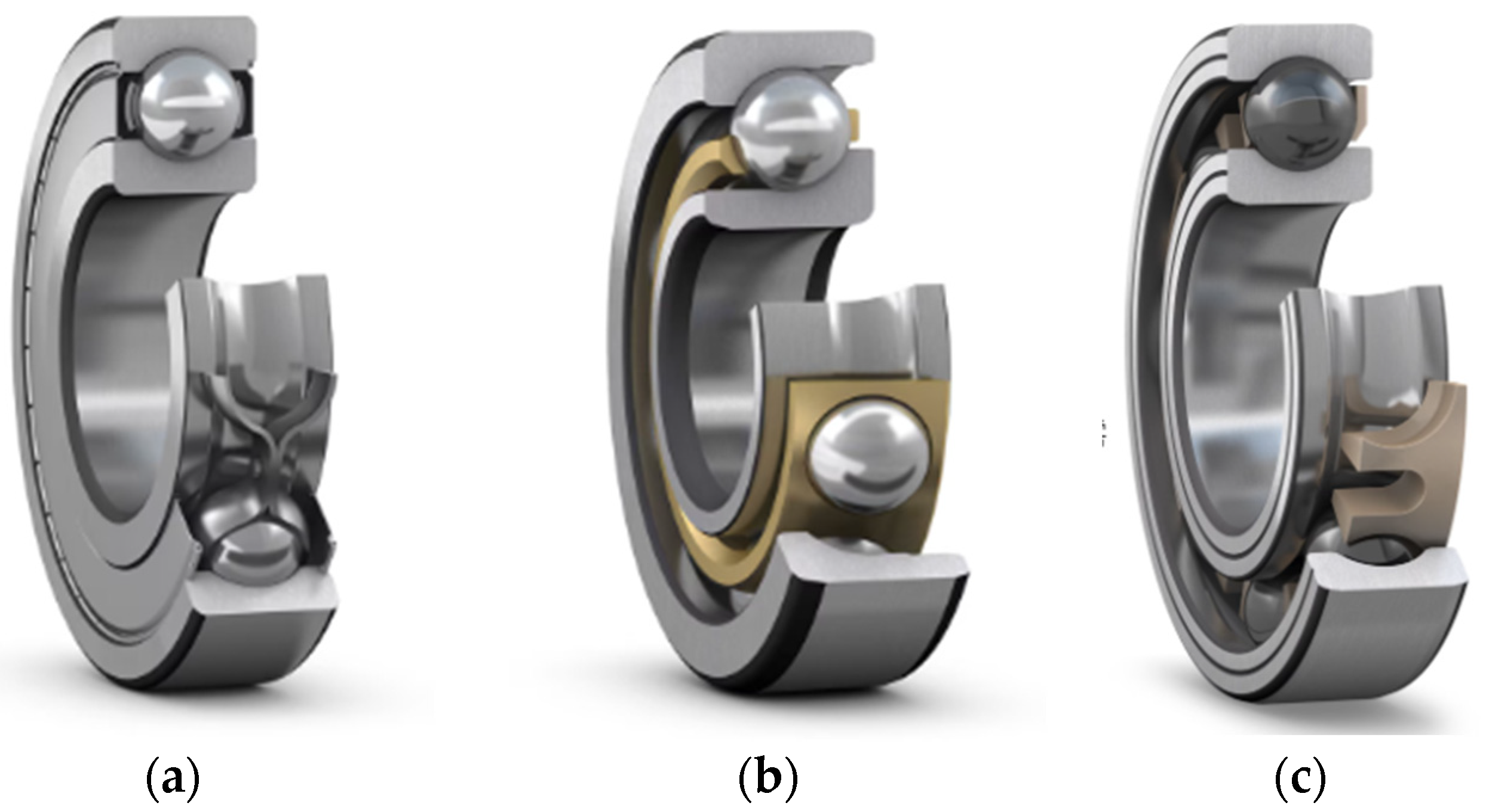
The most common types of bearings include the following: (a) Deep-groove ball bearings are one of the most commonly used bearing types, capable of handling radial loads and certain amounts of axial loads. Since the rotor in a PMSM typically needs to be supported at the center of the stator and allowed to rotate freely, deep-groove ball bearings are a common choice. (b) Angular contact ball bearings can withstand higher axial loads, and due to their contact angle design, they can handle higher rotational speeds and reduced vibration. In some high-performance or demanding PMSM applications, angular contact ball bearings may be selected. (c) Hybrid ceramic deep-groove ball bearings: The use of ceramic balls reduces friction and wear, which can lead to lower operating temperatures, increased speed capabilities, and an extended service life compared to all-steel bearings. They are often chosen for high precision, low noise operation, and resistance to corrosion, making them ideal for applications such as electric motors, high-speed machinery, and environments where conventional steel bearings might not perform as well due to friction, heat, or chemical exposure.

It is important to note that the specific bearing type and specifications depend on the design, application requirements, and operating conditions of the PMSMs. Rolling bearings are widely used in PMSMs due to their advantages such as having a low friction coefficient, high load bearing capacity, and high operating precision. Here are several commonly used types of rolling bearings in Figure 2 [28].

The advent of new bearing materials has given rise to a multitude of methods, including the one discussed by Saucedo-Dorantes, J.J., namely the use of image recognition for the identification of surface defects to pre-emptively address faults in full-ceramic bearings, employing an algorithm that combines the Gaussian filter with the improved homomorphic filter [29]. D. Liao adopted the autoencoder technique, integrating time-domain, frequency-domain, and time–frequency-domain technologies for data mining [30]. These two references hold significant reference value in the domain of fault diagnosis for new material bearings. However, the experimental validation conducted in this article pertains to metal bearings.

In the construction of electric motors, bearings play a role not only in supporting the rotation of the rotor but also in achieving the alignment of the rotor. Therefore, the working performance and condition of the bearings affect the normal operation of the motor. As shown in Figure 2, the main components of the bearing include the following: the outer ring, inner ring, balls, and cage. The main forms of bearing failures include scoring, wear, fracture, cage damage, corrosion, etc.

2.2. Bearing Faults Theory Analysis

When a fault exists on the outer race of the bearing and the bearing is rotating, the rollers will strike the fault repetitively and generate mechanical impulses. The impulses will excite the resonance of the system, and the resonance will be damped out quickly due to the structure damping. So, the vibration measured will contain these impulses with damped oscillations. The repetition frequency of these impulses, which is known as the fault characteristic frequency of the outer race, is related to the structure of the bearing geometry and the rotational frequency of the shaft. Equation (1) is the fault characteristic frequency of the outer race [31,32]. $N$ is the number of rollers, $f_r$ is the rotating speed of the shaft, $d$ is the diameter of the roller, $D$ is the pitch diameter and $\alpha$ is the contact angle.

$$BFO={\displaystyle \frac{N}{2}}{f}_r(1-{\displaystyle \frac{d}{D}}\cos (\alpha ))$$

(1)

The resonance demodulation detects the fault of the outer race by extracting the impulses associated with the fault characteristic frequency, as in Figure 3.

The first step of resonance demodulation is filtering the vibration signal with a band-pass filter whose pass band is the resonance frequency range of the system. The filtering process acquires the resonance signal caused by the bearing fault. A finite impulse response (FIR) filter can be utilized and the filtering process calculates the convolution of the filter and the vibration data. So, the filtering process can be realized via the convolution process without bias in a CNN model.

The second step of resonance demodulation is the amplitude demodulation of the filtered signal. The demodulation process acquires the envelope of the resonance signal. Demodulation methods, such as squaring the signal or Hilbert transform, are utilized. A rectification followed by a low-pass filter is also utilized for AM signal demodulation in a radio system. The rectification process can be presented by the ReLU layer in a CNN model, and the low-pass filter can also be realized by a convolution process without bias.

The Fourier transform is applied to the envelope signal, and amplitude at the fault characteristic frequency point in the envelope spectrum is extracted. If the amplitude is larger than a threshold, the bearing will be considered to be faulty. An alternative method can be utilized to achieve the same goal. When the rotating speed is constant, the fault characteristic frequency will be constant for a specified bearing. A narrow-band filter, whose center frequency is the fault characteristic frequency, can be utilized to filter the envelope signal. And the bearing will be considered faulty if the amplitude of the filtered signal reaches a threshold. So, the filtering process is a convolution process of CNNs without bias.

For the fault on the inner race and the roller of the bearing, the diagnosis processes are the same as the fault on the outer race. The fault characteristic frequencies of the inner race and the roller are Equations (2) and (3), respectively [1].

$$BFI={\displaystyle \frac{N}{2}}{f}_r(1+{\displaystyle \frac{d}{D}}\cos (\alpha ))$$

(2)

$$BSF=f_r{\displaystyle \frac{D}{d}}(1-{({\displaystyle \frac{d}{D}}\cos (\alpha ))}^2)$$

(3)

The pass band of the band-pass filter is difficult to select because the resonance frequency range of the system is usually unknown and selecting an optimized pass band requires experience and expert knowledge. The threshold of the amplitude at the characteristic frequency point in the envelope spectrum is also difficult to select.

As the resonance demodulation proves to be effective, a CNN with the structure of the resonance demodulation should be able to identify the bearing fault after training. The structure is as shown in Figure 4.

The first CNN layer finds the resonance frequency range of the system, and the ReLU activation demodulates the signal. The second CNN layer is a low-pass filter, and the envelope of the impulses caused by bearing fault is acquired. The activation of this layer is the linear activation, and the stride is 10 to reduce calculation cost. The next layer contains three convolution kernels that act as the narrow-band filters and can extract the vibration component with fault characteristic frequency of the outer race, the inner race, and the roller, respectively. And then, two fully connected layers are utilized for classification.

As the narrow-band filter is related to the rotating speed, the model will change when the rotating speed changes. The CNN model should be trained and tested with the data sampled at the same rotating speed.

3. Experiments

The bearing fault datasets from Case Western Reserve University (CWRU) [33] are utilized to validate the CNN model based on resonance demodulation.

3.1. Experiments with CWRU Data

The vibration signals of CWRU datasets are sampled in different bearing health conditions and the sample frequency is 12 kHz. The bearing health conditions include normal conditions, inner race faults, outer race faults, and roller faults. Each fault type contains different degrees of fault severity represented by the fault diameter.

The fault characteristic frequency for the outer race is 3.5848-fold of the rotating speed of the shaft in Hz; it is 5.4152-fold of the rotating speed for the inner race and 4.7135-fold of the rotating speed for the roller.

The data at the drive end are utilized to identify the drive-end bearing faults. The samples of different datasets for model training are prepared as follows. The starting point of each sample is randomly selected in a vibration data stream, and the following 12,000 data points are taken out as one sample of the corresponding dataset. There are 3994 samples for each rotating speed. The details of the datasets are in

Table 1. CWRU datasets for training and testing the CNN model.

Faults Type	Fault Diameter (mm)	Label	Sample Number
normal	-	normal	1000
roller fault	0.178	roller fault	250
roller fault	0.356	roller fault	250
roller fault	0.533	roller fault	250
roller fault	0.711	roller fault	250
inner race fault	0.178	inner race fault	250
inner race fault	0.356	inner race fault	250
inner race fault	0.533	inner race fault	250
inner race fault	0.711	inner race fault	250
outer race fault at 3 o’clock	0.178	outer race fault	142
outer race fault at 6 o’clock	0.178	outer race fault	142
outer race fault at 12 o’clock	0.178	outer race fault	142
outer race fault at 6 o’clock	0.356	outer race fault	142

. Different CNN models are trained and tested with data sampled at four different rotating speeds of 1797 rpm, 1772 rpm, 1750 rpm, and 1730 rpm. The dropout method is applied to each convolutional layer with a dropout rate of 0.2. In total, 70% of the samples in the datasets of different rotating speeds are selected randomly for training and the rest of the samples are utilized for testing.

For each CNN model at different rotating speeds, after training for 100 epochs in total, the loss of the network converges in general. The accuracy of CNN models for different rotating speeds is all 100%.

3.2. Experiments with IMS Data

For the datasets of IMS, the vibration signals are sampled at a constant rotating speed of 2000 rpm and the sampling frequency is about 20 kHz. This is based on a run-to-failure test of bearings under normal conditions. Four Rexnord ZA-2115 bearings (Rexnord Group, Milwaukee, WI, United States) are installed, and two accelerometers are installed on each bearing housing. The vibration signal records are collected every 10 or 5 min and 20,480 points are collected each time for each channel. The same experiment is repeated three times. At the end of the first experiment, the inner race defect in bearing 3 and a rolling element defect in bearing 4 occur. At the end of the second experiment, outer race failure occurs in bearing 1, and at the end of the third experiment, outer race failure occurs in bearing 3.

The fault characteristic frequency of the outer race is 236.40 Hz, and it is 296.93 Hz for the inner race and 279.83 Hz for the roller.

The structure of the CNN model is the same as in Figure 4. The data of bearing 3 in the last four records before failure in the first experiments are utilized for preparing the inner race fault data and those of bearing 4 are for roller fault data. The data of bearing 1 in the last four valid records before failure in the second experiment and data of bearing 3 in the last four valid records before failure in the third experiment are utilized for preparing the outer race fault data. The data of all bearings in the first records in different experiments are utilized for preparing the normal data. For each sample utilized for training and testing the CNN, the start point of a sample is selected randomly in the vibration signal stream and the following 12,000 points are taken out as one sample of the corresponding dataset. Finally, the datasets contain 1000 samples labeled as inner race fault, 1000 samples as outer race fault, 1000 samples as roller fault, and 1000 samples as normal data. In total, 70% of the samples in the datasets of different rotating speeds are selected randomly for training and the rest samples are utilized for testing.

The same experiments are repeated 10 times. The loss of the networks converges in general after training for 200 epochs in total, and the minimum accuracy of the CNN model is 99.7%.

Experiments on different bearing fault datasets prove that the CNN model based on resonance demodulation can identify different bearing faults.

4. Analysis and Optimization

4.1. Analysis of the Model of CWRU Datasets

The weights of the CNN model are analyzed. The magnitude responses of the weights in the first convolutional layer are as Figure 5. They are band-pass filters whose pass bands are about 3600~3900 Hz. This can be regarded as the resonance frequency of the system recognized by the CNN model.

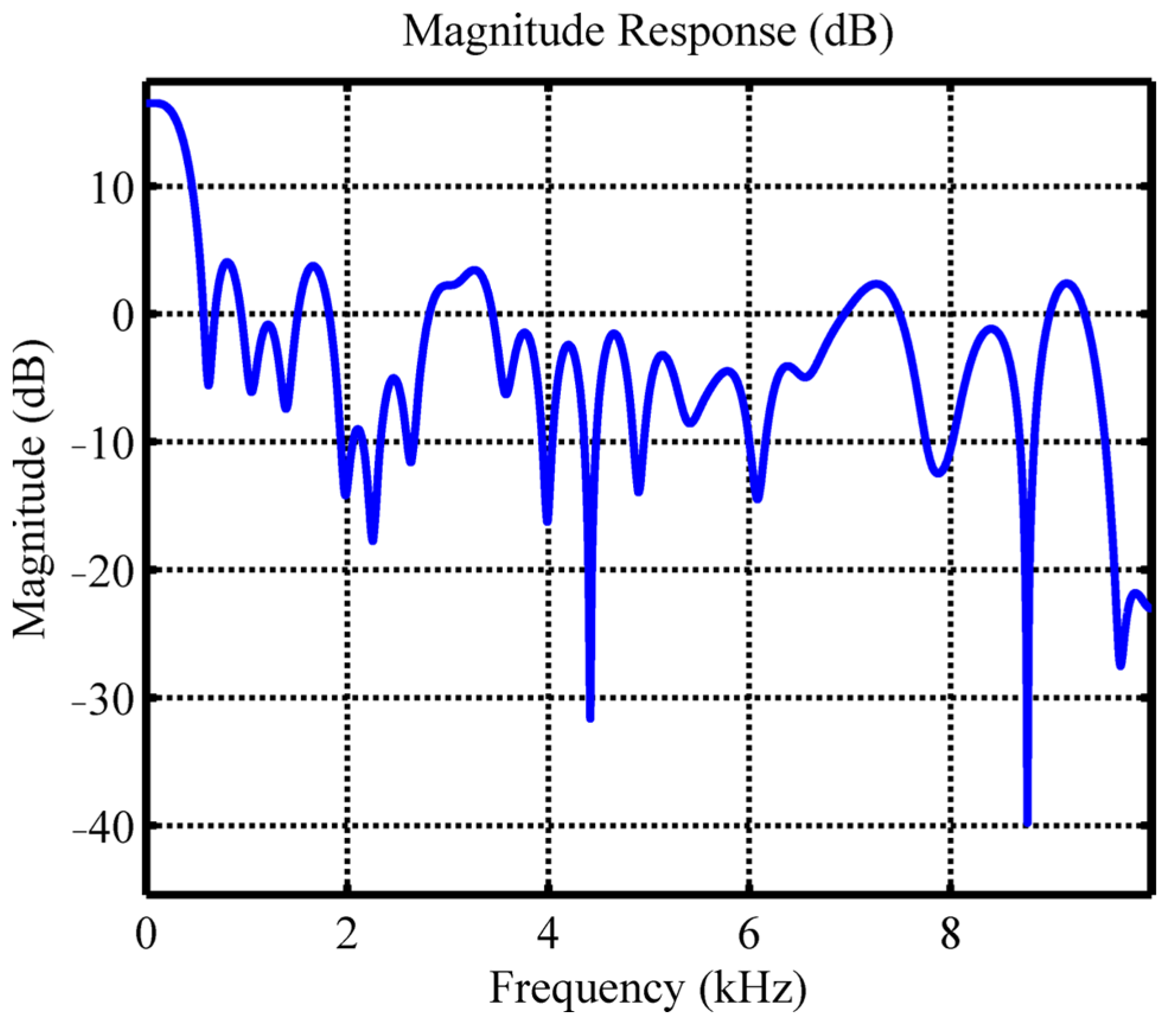
After the ReLU process, the second convolutional layer is applied. The magnitude responses of the second convolutional layer are in Figure 6. They are band-pass filters and the −3 dB band is about 80 Hz to 280 Hz. The high-frequency component of the input signal is filtered and the fault characteristic frequencies for different bearing faults are retained. According to the resonance demodulation method, the demodulation process can be realized by the rectification followed by a low-pass filter. As the low-pass filter in the demodulation process filters the high-frequency component and retains the signals whose frequencies are the fault characteristic frequencies, the function of the low-pass filter in the demodulation process is the same as the band-pass filter realized in the second convolutional layer of the CNN model.

The first two convolutional layers are consistent with the resonance demodulation method.

The third convolutional layer contains three FIR filters. For the CNN model trained with the rotating speed of 1793 rpm, one filter in this layer has a peak at the outer race fault characteristic frequency point in the magnitude response. Compared to other filters, the magnitude of data with outer race bearing fault is relatively large when filtered with this filter. This filter can be regarded as the filter that extracts the feature of the outer race fault. Another filter has a peak at the inner race fault characteristic frequency points in the magnitude response; so, it is related to the inner race fault. The third filter has no obvious peak at the roller fault characteristic frequency point in the magnitude response, but when the data of roller bearing fault is presented, the amplitude of the data filtered by this filter is larger than other filters. So, the third filter is related to the roller fault.

Filters in the third layer of other CNN models with different rotating speeds are similar to those of the CNN model of 1793 rpm. Figure 7, Figure 8 and Figure 9 are magnitude responses of filters for outer race fault, inner race fault, and roller fault, respectively, at different rotating speeds. The process of the CNN at the third layer is basically consistent with the resonance demodulation method.

For the filters related to the roller bearing fault, other features are possibly extracted for data classification as the feature at the roller fault characteristic frequency point is not obvious. For the filters related to the inner race bearing fault or outer race bearing fault, other peaks can also be observed in the magnitude responses. The possible reason for this is that, in addition to the characteristics of the feature frequency points, other features are also used for data classification, some of which are related to bearing faults, while others are unrelated to the characteristics of bearing faults.

4.2. Analysis of the Model of IMS Datasets

The analyzing process of the CNN model of IMS datasets is similar to that of the CWRU datasets. The same experiments are repeated 10 times. For the result of the first experiment, the amplitude response of the weights in the first convolutional layer is as Figure 10, and it is a band-pass filter centered around 5000 Hz. The amplitude response of the second layer is in Figure 11, and it is a low-pass filter. The first two layers are the same as the resonance demodulation method.

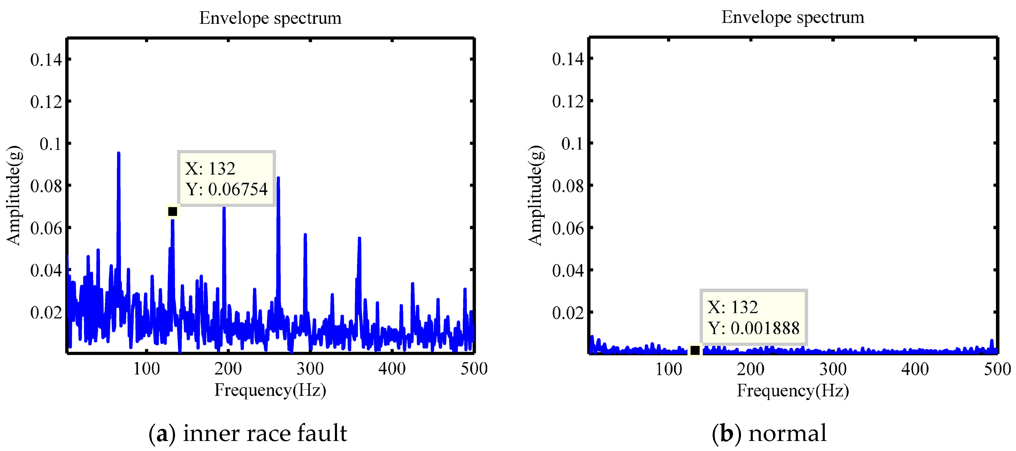
For the result of the first experiment, the amplitude responses of filters in the third layer are in Figure 12. In the third layer, there exists a filter that has a peak near the outer race fault characteristic frequency in the amplitude response. Another filter has a peak near the inner race characteristic fault frequency (about 296 Hz) in the amplitude response and the peak is not obvious; meanwhile, the highest peak in the amplitude response is at around 131 Hz. The envelope spectra of data with different bearing faults are in Figure 13, and the amplitude at 131 Hz of inner race fault data is significantly larger than the others. So, the CNN model utilizes this feature to classify the data of inner race faults. All filters have no peak at the roller fault characteristic frequency so the roller bearing fault data are classified by other features.

For the results of all repeated experiments, seven of them have a band-pass filter in the first convolutional layer and a low-pass filter in the second convolutional layer while the other three results do not. The reason for this may be that other processes different from resonance demodulation can also classify different datasets. For the CNN models whose first two layers are consistent with the resonance demodulation, the amplitude responses of the filters in the third convolutional layer are not the same. Some of them have peaks at the fault characteristic frequency points while others do not. Features different from the fault characteristic frequencies are utilized for data classification and these features may not relate to the bearing faults.

4.3. Optimization of the Training Process

When the features not related to the bearing faults are utilized for classification, the classification might fail if these features change. Another fault diagnosis test is conducted with the CNN model utilizing the CWRU datasets. The datasets are described in

Table 2. Datasets whose sampling conditions of the training and testing datasets are different.

Faults Type	Fault Diameter (mm)	Label	Used in Datasets	Sample Number
normal	-	normal	testing and training	1000
roller fault	0.533	roller fault	training	1000
inner race fault	0.178	inner race fault	training	1000
outer race fault at 12 o’clock	0.178	outer race fault	training	1000
roller fault	0.028	roller fault	testing	1000
inner race fault	0.533	inner race fault	testing	1000
outer race fault at 12 o’clock	0.533	outer race fault	testing	1000
outer race fault at 6 o’clock	0.178	outer race fault	testing	1000

. The training dataset contains data collected with an inner race fault of 0.178 mm, outer race fault of 0.178 mm, and roller fault of 0.533 mm while the testing dataset contains data collected with an inner race fault of 0.533 mm, outer race fault of 0.533 mm, and roller fault of 0.711 mm. The sample condition of the testing datasets is different from that of the training datasets, and because different bearings are used and the bearings are reinstalled, the installation error and the machining error are different. This test further accords with the practical situation because the data to be classified are usually not previously acquired and are not in the dataset for training.

As presented in

Table 3. Testing results without optimization and with optimization.

Rotating Speed (rpm)	Testing Datasets	Accuracy without Optimization (%)	Accuracy with Optimization (%)
1793	roller fault	27.4	100
1793	inner race fault	0	100
1793	0.533 mm outer race fault at 12 o’clock	99.4	100
1793	0.178 mm outer race fault at 6 o’clock	100	100
1772	roller fault	18.4	100
1772	inner race fault	98	100
1772	0.533 mm outer race fault at 12 o’clock	22	100
1772	0.178 mm outer race fault at 6 o’clock	100	100
1750	roller fault	88.5	100
1750	inner race fault	0	100
1750	0.533 mm outer race fault at 12 o’clock	7	100
1750	0.178 mm outer race fault at 6 o’clock	53.9	100
1730	roller fault	0	100
1730	inner race fault	0	53.2
1730	0.533 mm outer race fault at 12 o’clock	100	100
1730	0.178 mm outer race fault at 6 o’clock	100	100

, the testing results show that the model cannot identify the bearing fault of the testing dataset accurately in many cases. One possible reason is that the CNN model tries to find differences in datasets with different labels during the training process. The differences in the different datasets contain not only the bearing faults but also other features not related to the bearing faults. The different features not related to the bearing faults may be caused by different working conditions such as the temperature, the pressure, the installation error, or the machining error. The trained CNN model may fail to classify a new dataset correctly when the features not related to the bearing fault change while the bearing fault condition does not change. And, in practical situations, it is difficult to ensure that the features not related to the bearing faults do not change when a new dataset is acquired.

One solution is trying to collect enough data with all working conditions to train the CNN model. But, the data collection process is difficult, especially for a newly designed machine.

Another solution is utilizing the domain adaptation method, and this method is proven to be effective [21,22,23,24,25,26,27,28,29]. However, the datasets in the target domain are usually used during the training process for the domain adaptation method. So, when a dataset in a new target domain is acquired, the deep learning model needs to be retrained. This increases the calculation cost.

According to the theory of resonance demodulation method, the training process is optimized to increase the generalization of the CNN model. The second convolutional layer acts as a low-pass filter for demodulation, the weights of this layer are initialized as an FIR low-pass filter with the pass band lower than 400 Hz, and the output of this layer is the envelope signal.

The third convolutional layer contains three filters. The filters are initialized as narrow-band filters whose center frequencies are the fault characteristic frequencies of the outer race, the inner race, and the roller, respectively.

During the training process, the second and third layers are frozen. The training process only changes the weights of the first convolutional layer and the last two fully connected layers. The training process can be regarded as the process of finding the optimized resonance frequency range and optimizing the classification process of the last two fully connected layers.

The datasets described in Table 2 are utilized to test the optimized training process. And, four CNN models are trained with different narrow-band filters for four different rotating speeds. These results are in Table 3. The results show that the CNN models identify the different bearing faults much more accurately when the optimization process is utilized.

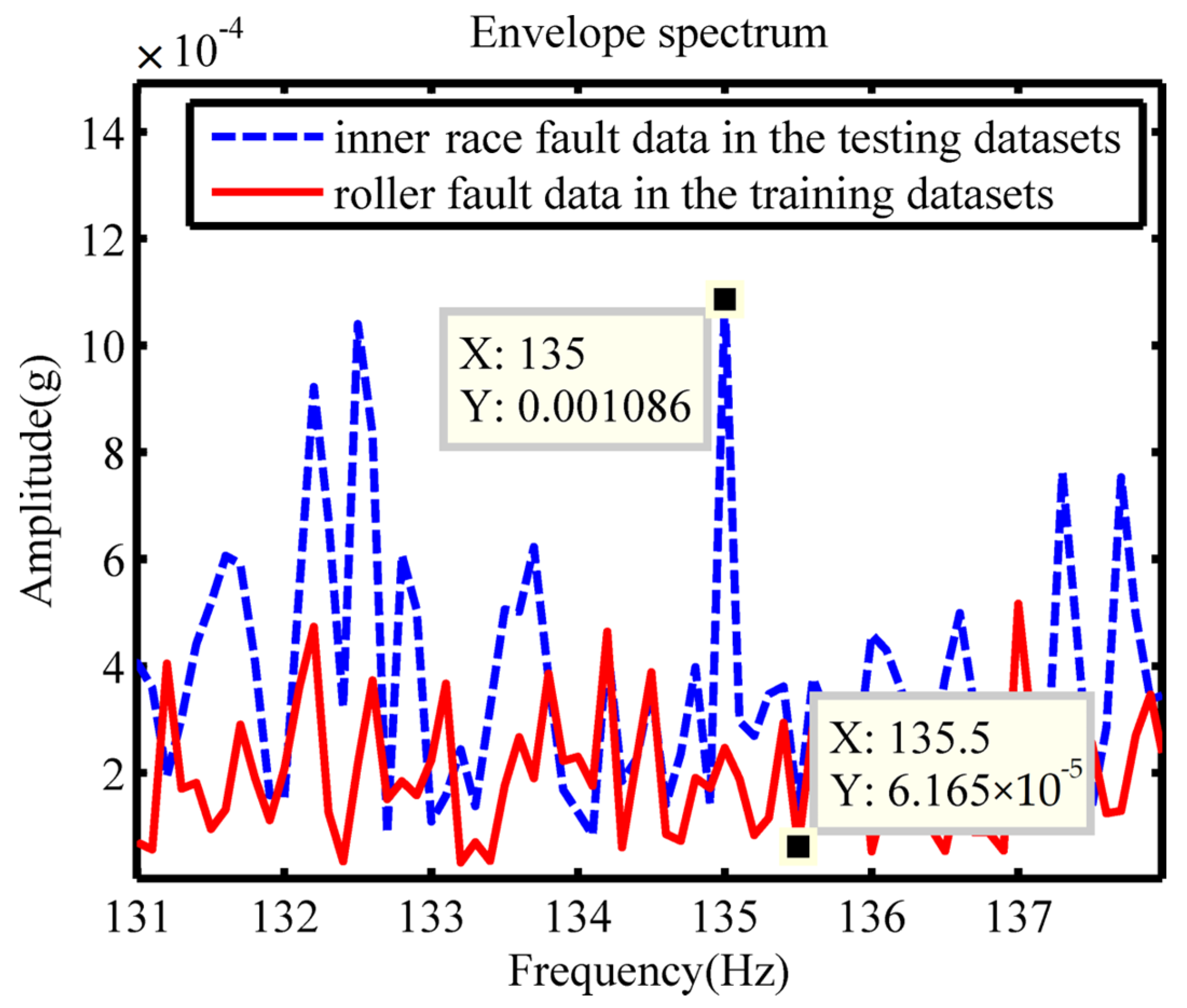
However, the results of the inner race fault identification are not accurate when the rotating speed is 1730 rpm, and all incorrect results classified the samples as the roller fault. The envelope spectrum of the vibration signal of roller fault data in the training dataset and inner race fault data in the testing dataset are analyzed. As in Figure 14, the envelope spectrum shows that there is no obvious amplitude peak at the roller fault characteristic frequency for the roller fault data in the training datasets; meanwhile, the inner race fault has a spectrum peak at this fault characteristic frequency. This result means that when the fault characteristic for the dataset utilized for training is not obvious, the accuracy of the CNN model might be affected by the noise signal whose frequency is the corresponding fault characteristic frequency.

The optimization process only utilizes the bearing fault feature at the fault characteristic frequency point to identify different bearing faults; the other features related to different bearing faults are ignored. So, the optimization process is suitable for the condition where datasets at different working conditions are not available. When enough datasets are collected, the CNN model should be trained without optimization.

5. Local Dataset Validation

To further validate the optimization effect of the CNN model, local experimental data were collected for testing. The speed was set to 30 Hz, with a sampling rate of 12.5 kHz and an effective load. The faulty bearing was an outer race fault (6 o’clock direction), with a fault characteristic frequency equal to 3.048 times the speed. To test whether the CNN model extracted the bearing fault features for classification, the following experimental tasks were conducted: vibration signals from both normal and faulty bearings at 30 Hz speed, with and without grinding of the bearings, were collected. This resulted in four sets of vibration data for the two classes of bearings at the same speed. The vibration data without grinding from the normal bearings were used as the training set for the normal samples; meanwhile, the vibration data with grinding from the faulty bearings were used as the training set for the fault samples in order to conduct a two-class classification of bearing conditions.

As shown in Figure 15, the fault diagnosis test bench for PMSMs is mainly composed of a permanent magnet synchronous motor, a motor controller, a coupling, a photoelectric speed sensor, a vibration sensor, etc.

The test bench has a power of 2.5 kw and a maximum speed of 8000 rpm. The parameters of the local test bench are displayed in

Table 4. Parameters of the local equipment and instrument.

Parameter Types	Value
Motor Power	2.5 kW
Maxim Speed	8000 rpm
Types of Bearing Faults	Outer, Inner, Rolling element
Sampling Frequency	102.4 kHz (max)
Sampling Accuracy	24 bit
Vibration Sensor	IEPE
Sensor Frequency Range	10 kHz

. The main sensors include a speed sensor, a current sensor, and a vibration acceleration sensor. The acquisition equipment transmits the sensor signals to the computer acquisition software through the acquisition card, enabling online processing and the saving of the data.

The experimental data were processed as follows: a random sample of 12,500 data points of vibration data were taken as one sample, with 5000 samples extracted from each group, resulting in 10,000 samples for both the training and testing sets. In all, 70% of the data were randomly selected for training, while the remaining data were used for validation. The CNN model used the same model as in Figure 4, with the third layer having only a single convolutional kernel. After 100 training iterations, the training loss converged. Figure 16 presents the intermediate process output, layer by layer. The test results showed that the model achieved an accuracy of 100% on the training set but only 99.22% on the testing set, mainly misclassifying 77 samples of normal bearings with grinding as faulty bearings, as in Figure 17 and Figure 18. This was due to the CNN model extracting features other than the bearing fault features during the training process, leading to misclassification.

6. Conclusions

Due to its advantages such as high torque density, high power density, and small size, PMSMs have been widely used in electric vehicles and traction systems for rail transit. However, due to the harsh working environment of PMSMs, they are prone to various mechanical and electrical failures. Among them, bearing faults are the most common type of failure in PMSMs. Therefore, the diagnosis and condition monitoring of PMSM bearings have become a research hotspot for scholars worldwide.

In this article, a physical explanation of a deep learning model for bearing fault diagnosis is presented. The relationship between 1-D CNN and the resonance demodulation method is analyzed. A CNN model is established according to the resonance demodulation method. Experiments on different bearing fault datasets are conducted and the results show that the CNN model can identify different bearing faults at a constant rotating speed. The weights of the CNN model indicate that the CNN model is basically consistent with the resonance demodulation method. An optimized training process is presented. The optimization can increase the accuracy of the CNN model for the bearing fault datasets sampled in a different condition, which is not presented in the training datasets. The experimental results demonstrate that the CNN model can identify various types of bearing faults. The analysis of the trained CNN model and its intermediate outcomes indicates that the CNN model aligns with the resonance demodulation method.

The primary contribution of this article is its success in forging a link between traditional resonance demodulation and contemporary CNN methodologies. While the former is grounded in well-defined physical principles, the latter leverages the power of machine learning to harness the full potential of data. The article delves into the underlying commonalities of the physical models inherent in both these approaches. It substantiates the efficacy of fault diagnosis by offering a blend of theoretical insights and empirical evidence, thereby validating the robustness of the proposed diagnostic methods.

According to the theory of the resonance demodulation method, the CNN model presented can identify bearing faults at a constant rotating speed. This model can be applied to the rotating machine, which works at a constant rotating speed and has a working state with a constant rotating speed, in avenues such as the ground idle state of the aero engine.

Another application of the CNN model is to find the optimized band-pass filter for the resonance frequency range. That is training that the CNN model with the optimized process presented. Then, utilizing the weights of the first convolutional layer as the band-pass filter in the traditional resonance demodulation method can be applied. If the resonance frequency range changes a little while the rotating speed changes, the weights can be used at different rotating speeds.

Through the research in this article, it is further demonstrated that utilizing deep learning models such as CNNs, in conjunction with traditional analytical methods, significantly enhances the efficiency of bearing fault diagnosis.