Active Disturbance Rejection Control of Permanent Magnet Synchronous Motor Based on RPLESO

Abstract

In view of the problem of the low-speed jitter of household lawn mowers driven by a permanent magnet synchronous motor (PMSM) at low speeds and high torque, and the complicated parameters of traditional non-linear active disturbance rejection controllers, a partially optimized linear active disturbance rejection control (LADRC) driving PMSM strategy is proposed. First, the linear extended state observer (LESO), which bears a significant burden in terms of speed and load estimation in active disturbance rejection control, is optimized by reducing its order to improve the anti-disturbance performance of the active disturbance rejection controller within a limited bandwidth. Secondly, the reduced-order parallel linear extended state observer (RPLESO) is obtained by optimizing the parallel structure of the order-reduced LESO, which improves the control precision and robustness of the system. Through a simulation and experimental verification, the optimized LADRC control of the PMSM system is shown to improve the parameter adjustability, speed estimation precision and system robustness.

1. Introduction

Traditional non-road fuel vehicles, represented by domestic lawn mowers, have problems such as high power consumption, serious pollution and loud noise. Under the “two-carbon” strategic goal of “carbon peak” and “carbon neutrality”, the transformation of non-road fuel vehicles into electric power vehicles is an important means to deal with a series of problems, such as air pollution control, energy conservation, emission reduction and the energy crisis. Non-road vehicles have the characteristics of a narrow driving range, poor road conditions, uneven road surfaces and short driving distances [1], while ordinary motors are unable to meet the requirements of the unique working conditions. The permanent magnet synchronous motor (PMSM) is widely used in non-road electric vehicles, with its advantages of a simple structure, high power density, high operating efficiency, small size, large overload capacity, small moment of inertia and small torque ripple [2]. Therefore, the construction of motor speed regulation control systems with PMSMs as the core and in line with the complex non-road working conditions has become the research goal in this field. Most control methods in the traditional PMSM vector control system use PI controllers. The most common type is vector control. Although this controller can eliminate the dependence on a precise mathematical model of the controlled object, a contradiction exists between the system rapidity and overshoot [3]. When the PMSM system is subjected to internal and external periodic and aperiodic disturbances, such as speed fluctuations, sudden changes in load, parameter perturbations, the dead-time effects of inverters and sampling errors of the stator current, it is unable to ensure the high-precision control of the motor speed. To solve these problems, scholars at home and abroad have proposed advanced PMSM control algorithms, including sliding mode control [4], active disturbance rejection control (ADRC) [5], model prediction control [6], neural network control [7] and artificial intelligence control [8].

Initially proposed by Han Jingqing [9], ADRC has become a research hotspot at home and abroad since it does not depend on a precise system model and has high disturbance resistance capabilities. ADRC consists of three parts: a trace differentiator (TD), an extended state observer (ESO) and nonlinear state error feedback (NLSEF). The TD is used to arrange the transition process, reduces or avoids overshoot and provides high-quality input. The ESO is used to observe the internal and extended states to improve the controllability of the system. NLSEF is used to provide an effective control quantity. Because ARDC does not depend on a precise mathematical model of the controlled object and its structure is relatively fixed, it can reduce the external disturbance and internal uncertainty and alleviate the strong coupling and nonlinear characteristics of the motor, and it has the advantages of a strong anti-interference ability, small overshoot, high precision, strong robustness and a wide application range [10]. At the same time, ARDC also has many shortcomings, such as large algorithm parameters, a high demand for disturbance modeling, delays in computation and the increased consumption of computing resources. In order to reduce the difficulties in parameter adjustment and the number of system control parameters, linear active disturbance rejection control (LADRC) was proposed by Gao Zhiqiang et al. [11], which simplifies the structure of the auto-disturbance rejection controller. Furthermore, it proposes to adopt the frequency domain analysis method in classical control theory and a linear extended state observer (LESO) and linear state error feedback (LSEF) to tune the parameters of ADRC, so that the number of LADRC parameters is reduced to two. These are the controller bandwidth and observer bandwidth, which are closely related to the performance of the closed-loop system and greatly reduce the difficulty in the parameter tuning of nonlinear ADRC [12,13]. A single-winding bearingless flux-switching PMSM in linear ADRC with model compensation has been designed. The LESO and error feedback control rates have been implemented and compared to traditional PID control, demonstrating stronger anti-interference abilities [14]. Ref. [15] overcomes the non-smooth nature of the nonlinear function in the auto-disturbance controller, and an improved first-order ADRC is used in the machine control system to observe and feedforward the disturbance of the system through the extended state observer. Ref. [16] uses ADRC to control the speed only, but the state observer in ADRC also estimates the back-EMF, which is sent to a phase-locked loop (PLL) in order to obtain the final estimated speed and position. Refs. [17,18] only use ADRC and a speed estimation method based on a sliding mode observer (SMO) simultaneously. Ref. [19] proposes a simplified ADRC controlling both the speed and current. A few works, like [20], design basic two-order ADRC controllers for PMSMs. Therefore, LADRC can be easily applied to industrial control.

Taking the PMSM as the research object, this paper proposes an improved LADRC control strategy by analyzing its topological structure, its working principle and the operating conditions of off-road vehicles. Firstly, the disturbance of the speed loop is analyzed, and it is concluded that aperiodic disturbances, such as the speed and sudden changes in load, have the most prominent influence on the system. In order to improve the speed accuracy and robustness of the PMSM speed control system, the LESO, with a large estimated burden in the LADRC controller, is reduced in order. Instead of estimating the feedback speed calculated by the encoder, the load disturbance of the system is accurately estimated and fed back to the system, which improves its anti-disturbance ability. Then, the LESO with a reduced order is optimized in a parallel structure, which not only retains the advantage of the easy tuning of the LADRC parameters but also improves the observation precision and anti-disturbance ability of the controller. Through a simulation and experimental verification, the optimized ESO with a reduced-order parallel structure is shown to exhibit higher speed observation accuracy, tracking performance and system robustness, and it can effectively solve the problem of the jitter of domestic lawn mowers at low speeds.

2. The Mathematical Model of the PMSM and LADRC

2.1. The Basic Mathematical Model of the PMSM

This paper selects a three-phase surface permanent magnet synchronous motor (SPMSM) as its research object. The mathematical model of the SPMSM in a two-phase rotating coordinate system $d–q$ based on three-phase stator stationary coordinate $A–B–C$ and two-phase stator stationary coordinate $\alpha –\beta$ is presented in Figure 1.

Considering the ideal mathematical modeling of the PMSM, we make the following assumptions: (1) we ignore the magnetic circuit saturation effect; (2) we ignore the hysteresis and eddy current loss; (3) the magnetic field space is sinusoidal. The voltage equation under the $\alpha –\beta$ stationary coordinate system is

$$u_{\alpha }=R_s{i}_{\alpha }+L_s\frac{d{i}_{\alpha }}{dt}-{\omega }_e{\psi }_f\sin {\theta }_e$$

(1)

$$u_{\beta }=R_s{i}_{\beta }+L_s\frac{d{i}_{\beta }}{dt}-{\omega }_e{\psi }_f\cos {\theta }_e$$

(2)

In the equation, $u_{\alpha }$, $u_{\beta }$ and $i_{\alpha }$, $i_{\beta }$ are the voltage and current of the $\alpha –\beta$ axis, respectively; $L_s$ is the stator inductance; $R_s$ is the stator resistance; ${\psi }_f$ is the magnetic chain of the rotor permanent magnet; ${\omega }_e$ is the electric angular velocity; ${\omega }_e=p_n{\omega }_r$, where $p_n$ is the pole logarithm of the motor and ${\omega }_r$ is the mechanical angular velocity; and ${\theta }_e$ is the rotor angular position.

The voltage equation in the synchronous rotating $d–q$ coordinate system is

$$u_d=R_s{i}_d+L_d\frac{d{i}_d}{dt}-{\omega }_e{L}_q{i}_q$$

(3)

$$u_q=R_s{i}_q+L_q\frac{d{i}_q}{dt}+{\omega }_e{L}_d{i}_d+{\omega }_e{\psi }_f$$

(4)

In the equation, $u_d$ and $u_q$ are the stator voltages of the $d–q$ axis; $i_d$ and $i_q$ are the stator currents of the $d–q$ axis; $L_d$ and $L_q$ are the stator inductance of the $d–q$ axis; and $L_d=L_q=L_s$. The torque balance and motion equations of the PMSM, respectively, are shown below.

Torque balance equation:

$$T_e=\frac{3}{2}{p}_n\left[{\psi }_f{i}_q+\left(L_d-L_q\right)i_d{i}_q\right]$$

(5)

Since there is $L_q=L_d$ in the SPMSM, the torque equation is

$$T_e=\frac{3}{2}{p}_n{\psi }_f{i}_q$$

(6)

The equation of motion is

$$T_L=T_e-J\frac{d{\omega }_e}{dt}-B{\omega }_r$$

(7)

$T_e$ is the electromagnetic torque; $T_L$ is the load torque; $J$ indicates the inertia; $B$ is the viscosity friction coefficient.

2.2. The Basic Mathematical Model of LADRC

In this paper, the basic mathematical model of LADRC is derived by taking a second-order system as an example. The general form of the differential equation of the second-order system is

$$\ddot{y}=-a_1\dot{y}-a_{0}y+w+bu$$

(8)

In the equation, $y$ and $u$ are, respectively, the output and input of the controlled object; $\omega$ is the system disturbance; $a_0$ and $a_1$ are unknown coefficients; and $b$ is the controller gain. Combining Formulas (7) and (8), the equation of motion can be converted into

$$\left\{\begin{array}{l}{\dot{\omega }}_r=a(x)+b_{0}u\\ y={\omega }_r\end{array}\right.$$

(9)

in which $a(x)=\frac{K_e(i_q-u)-T_L-B{\omega }_r}{J}+(b-b_0)u$ is the total system disturbance; $K_e=\frac{3}{2}{p}_n{\psi }_f$ and $b=\frac{K_e}{J}$ are the control gain; $b_0$ is an estimate of $b$.

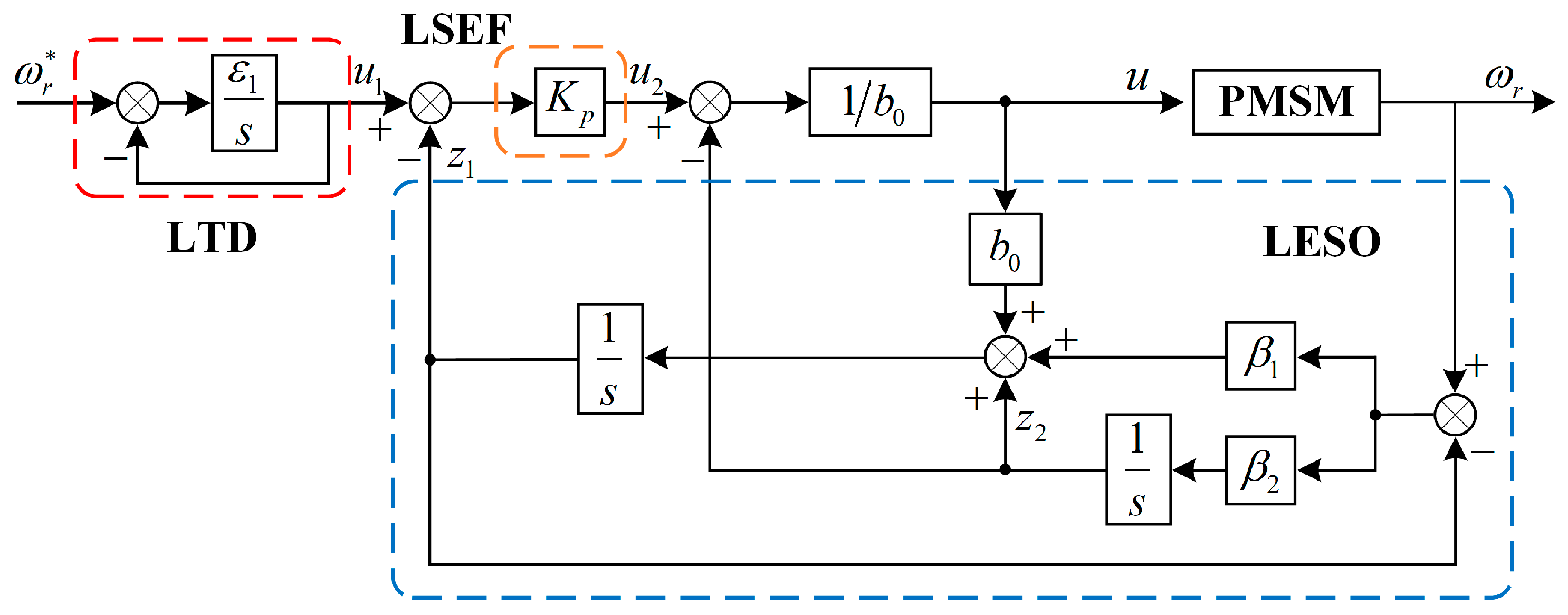
For the system shown in Equation (9), a linear trace differentiator (LTD) not only provides the transition process but also provides the corresponding differential signal of the transition signal, and the inertia link has a transition effect, so the first-order inertia link can be used to design the LTD for convenience.

$$\left\{\begin{array}{l}{e}_1=u_1-{\omega }_r^{\ast }\\ {\dot{u}}_1=-{\epsilon }_1{e}_1\end{array}\right.$$

(10)

$e_1$ is the observation error of the LTD; $u_1$ is the tracked input signal; and ${\epsilon }_1$ is the tracking factor (the time constant of the inertial link).

The mathematical model of the second-order LESO can be derived from Formula (9) as follows:

$$\left\{\begin{array}{l}{e}_2=z_1-{\omega }_r\\ {\dot{z}}_1=z_2-{\beta }_1{e}_2+b_{0}u\\ {\dot{z}}_2=-{\beta }_2{e}_2\end{array}\right.$$

(11)

$e_2$ is the observation error of the LESO; $z_1$ is the tracking value of rotational speed ${\omega }_r$; $z_2$ is the observation value of the disturbance; ${\beta }_1$ and ${\beta }_2$ are the gain coefficients of the observer.

The linear state error feedback for the system shown in Equation (9) can be designed as

$$\left\{\begin{array}{l}{e}_3=u_1-z_1\\ u_2=K_p(u_1-z_1)\\ u=(u_2-z_2)/b_0\end{array}\right.$$

(12)

$e_3$ is the observation error of the LSEF; $K_P$ is the proportional adjustment factor, related to the bandwidth of the system.

The final form of the LADRC controller can be obtained by combining the above Formulas (10)–(12):

$$u=\left[K_p({\omega }_r^{\ast }-{\omega }_r)-z_2\right]/b_0$$

(13)

The parameters that need to be fixed in the controller are ${\epsilon }_1$, ${\beta }_1$, ${\beta }_2$ and $K_P$. According to the LESO parameter configuration method in the literature [11], an appropriate observer bandwidth and controller bandwidth are selected to determine the convergence speed of the observer and controller, respectively, and we set parameters ${\beta }_1=2{\omega }_o$, ${\beta }_2={\omega }_o^2$, $K_P={\omega }_c$. Generally, when designed, ${\omega }_o$ is about 3–5 times that of ${\omega }_c$. The control block diagram of the speed control structure of the traditional LADRC is shown in Figure 2.

2.3. The Design of the Order-Reduced Parallel LESO

In the traditional LESO, not only the system disturbance value but also the feedback velocity ${\omega }_r$ is observed. In fact, in the speed loop of the servo system, the feedback speed signal can be precisely measured by the encoder, so the state feedback observer does not need to observe the speed signal. Moreover, the speed information obtained directly via the encoder can cause the speed feedback signal to be unaffected by the bandwidth of the observer. Therefore, a reduced-order linear extended state observer (RLESO) can be obtained by reducing the order of the above second-order extended state observer.

According to the above Equation (11), the equation of state is established as follows:

$$\left[\begin{array}{l}{\dot{z}}_3\\ {\dot{z}}_4\end{array}\right]=\left[\begin{array}{cc}0& 1\\ 0& 0\end{array}\right]\left[\begin{array}{c}{z}_3\\ z_4\end{array}\right]+\left[\begin{array}{c}1\\ 0\end{array}\right]b_{0}u+\left[\begin{array}{c}0\\ 1\end{array}\right]\dot{a}(t)$$

(14)

$z_3$ is the state variable of the rotation speed ${\omega }_r$; $z_4$ is the state variable of the total disturbance of the system $a(t)$. Since $z_3$ is known and $z_4$ is unknown, $z_4={\dot{z}}_3-b_{0}u$ is set, and a descending-order observer is constructed as follows:

$${\dot{z}}_2=-{\beta }_3(z_2-z_4)={\beta }_3({\dot{z}}_3-z_2-b_{0}u)$$

(15)

where ${\beta }_3$ is the bandwidth of the reduced-order observer.

In general, there will be measurement noise when the signal is measured directly by the sensor, and Equation (15) contains the differential term $z_3$, which is sensitive to noise. In order to suppress the influence of noise signals, the variable substitution method is used to change the above equation. We define a new state variable as follows:

$$z_5=z_4-{\beta }_3{z}_3$$

(16)

From Formulas (15) and (16), it can be obtained that

$$\left\{\begin{array}{l}{\dot{z}}_5=-{\beta }_3(z_5+{\beta }_3{z}_3+b_{0}u)\\ \widehat{a}(t)=z_5+{\beta }_3{z}_3\end{array}\right.$$

(17)

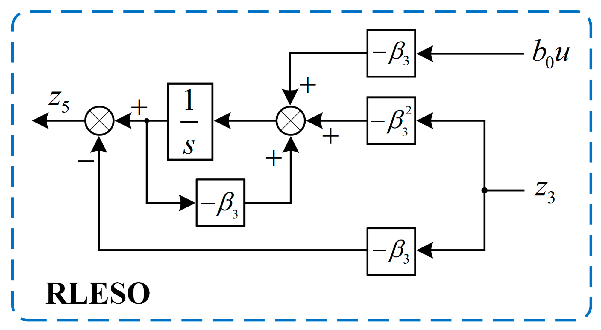
where $\widehat{a}(t)$ is the observed integrated disturbance. Equation (16) achieves the estimation of the total disturbance of the system $a(t)$ and has a better anti-interference capacity with regard to the system noise and better adaptability. The structure block diagram of the RLESO is shown in Figure 3.

Compared with nonlinear active disturbance rejection control, order-reduced linear active disturbance rejection control is more simplified in its parameter configuration, but, due to bandwidth limitations in actual observation, large observation errors will be generated, increasing the burden of the closed-loop controller [21]. In order to equip the observer with the ideal bandwidth, from the perspective of the hardware cost, system sampling frequency and sensor noise, this paper considers the parallel connection of two order-reduced LESOs to obtain a wider range of adjustable bandwidths and better observation performance without increasing the system cost or the adjustable parameters. Figure 4 shows the structural diagram of the reduced-order parallel linear extended state observer (RPLESO).

In order to simplify the design, both observers use the same parameters.

Table 1. Parameters of the control system.

Parameter	Numeric Value
LTD tracking factor ${\epsilon }_1$	8
Observer bandwidth ${\omega }_o$	2500
Controller bandwidth ${\omega }_c$	500
Controller gain $b_0$	12
Current ring controller $K_P$	17
Current ring controller $K_i$	5750

lists the system control parameters.

As shown in Figure 4, the system disturbance is divided into two parts: $z_5$ and $\widehat{a}(t)$.

$$a(t)=z_5+\widehat{a}(t)$$

(18)

Here, $z_5$ is the observed value of RLESO1 for the disturbance $a(t)$e, and $\widehat{a}(t)$ is the observed error of the disturbance.

When RLESO1 is subjected to a large disturbance, $z_5$ cannot be completely compensated for, so it is considered to compensate for the observation error $\widehat{a}(t)$ via the parallel RLESO2, so as to compensate for the total disturbance of the system more accurately. The basic principle of disturbance compensation is to transform the original system into a first-order integral system and construct a first-order integral system with $u_1$ as the input. The influence of the disturbance error on the system is the difference between the output of the integral system and that of the actual system, and $\widehat{a}(t)$ is accurately observed and offset by the parallel RLESO.

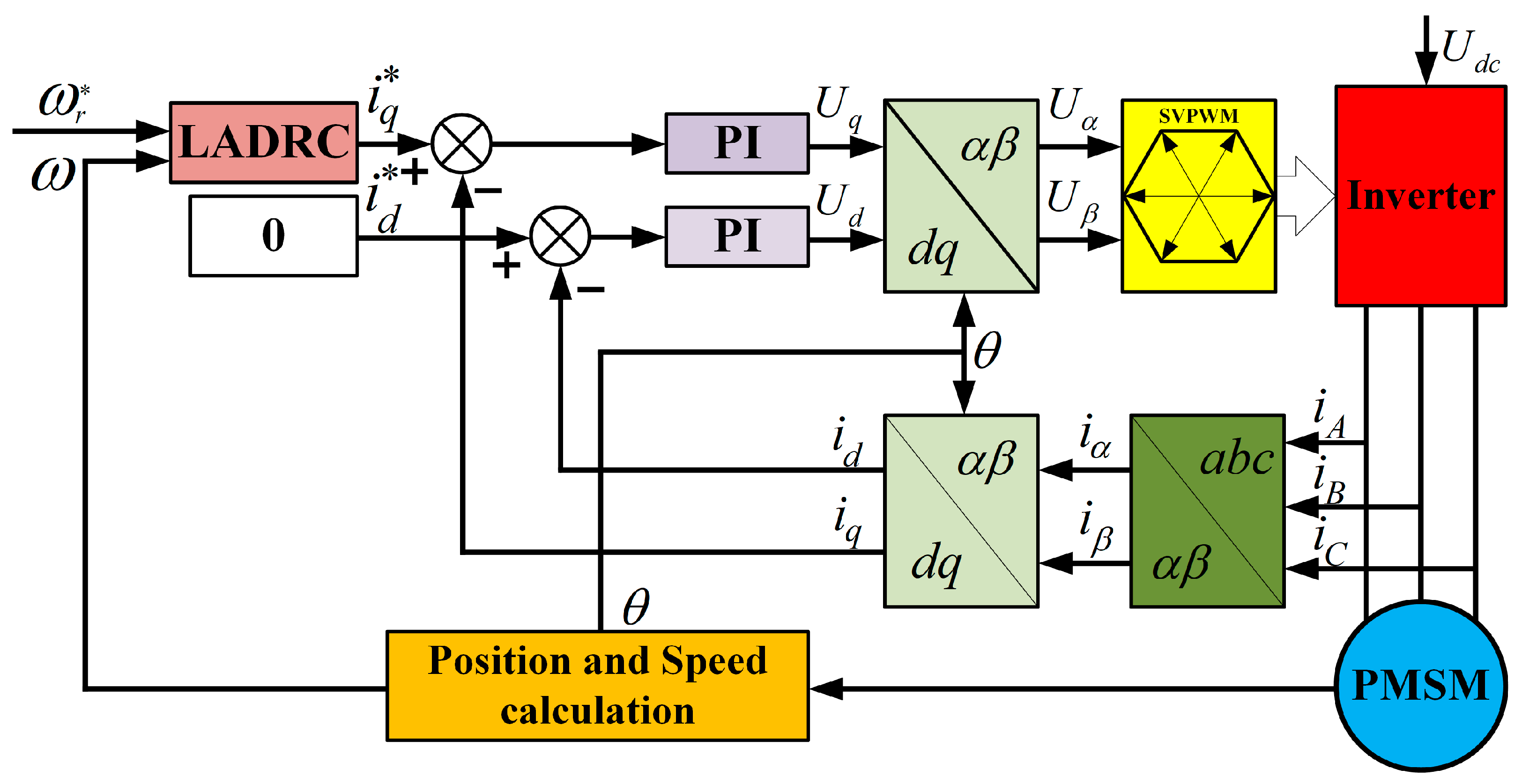
Based on the above design, where the current loop is controlled by the PI, the block diagram of the PMSM speed active disturbance rejection control system with the RPLESO designed in this paper can be obtained, as shown in Figure 5.

3. Simulation Analysis

In order to verify the effectiveness of the control strategy designed above, this system, as well as the traditional PI double closed-loop control system and the traditional linear ADRC speed governing system, as shown in Figure 5, asre built in MATLAB/Simulink ver. R2024a, respectively, for a simulation and comparative study. The research object of this paper is the driving motor (with a reducer) of the domestic lawn mower. The specific parameters of the driving motor are shown in

Table 2. Parameters of the permanent magnet motor.

Parameter	Numeric Value
Power rating$/\mathrm{K}\mathrm{W}$	2.2
Rated voltage$/\mathrm{V}$	72
Rated current$/\mathrm{A}$	32
Rated speed$/(r/\min )$	5500
Stator resistance$/\mathrm{\Omega }$	0.066
$d$ Axis inductance$/\mathrm{H}$	0.59
$q$ Axis inductance$/\mathrm{H}$	0.59
Number of pole pairs $P_n$	5
Rated torque$/(\mathrm{N}\cdot \mathrm{m})$	14.3
Linkage$/\mathrm{W}\mathrm{b}$	0.175
Moment of inertia$/(\mathrm{k}\mathrm{g}\cdot {\mathrm{m}}^2)$	2.48

.

3.1. Speed Tracking Simulation Experiment

The simulation experiment’s strategy is as follows: when the motor is unloaded, the initial reference speed is set to 500 r/min; the reference speed is set to 1200 r/min at 0.2 s; the reference speed is suddenly reduced to 1000 r/min at 0.4 s; and at 0.6 s, the reference speed is suddenly reduced to 400 r/min. The simulation results are shown in Figure 6. It can be seen from the local magnification diagram in the figure that both the control algorithm with the RPLESO designed in this paper and the traditional linear ADRC control algorithm have a faster response than the PI control. In terms of overshoot, the algorithm designed in this paper has a smaller overshoot than the traditional LADRC control algorithm, which is almost negligible. In terms of steady-state precision, the control algorithm proposed in this paper has a smaller steady-state error.

3.2. Simulation Experiment with Sudden Changes in Load

In order to verify the adaptability of the control strategy under sudden load changes, the following simulation experiments are designed. The motor starts with no load and the steady speed is set at 1000 r/min. When the motor reaches the steady speed, a load torque of 10 N·m is suddenly added at 0.1 s. When the rotational speed is stabilized, we remove the load at 0.3 s, and the system’s speed response curve is obtained, as shown in Figure 7.

Table 3. Speed overshoot.

Project	Rising	Loading	Unloading
RPLESO	0.288	0.077	0.083
LADRC	1.850	0.079	0.060
PI	0	0.642	0.637

Numerical units: %.

and

Table 4. Precision of steady-state speed.

Project	Loading	Unloading
RPLESO	0.001	0.001
LADRC	0.029	0.018
PI	0.070	0.005

Numerical units: %.

show the calculated values of the velocity overshoot and steady-state error.

As can be seen from Figure 7, the overshoot of the proposed control strategy is significantly reduced compared with that of the traditional LADRC when the speed is increased, while the overshoot of both methods is superior to that of the traditional PI control during loading and unloading. Table 3 shows that the maximum overshoot of the PI control reaches 0.642%. Compared with the traditional LADRC control and PI control, the control strategy proposed in this paper has the advantage of smaller overshoot during a speed increase. Table 4 shows the steady-state accuracy of the velocity after the load becomes stable. It can be seen that, compared with the traditional control strategy, the steady-state speed precision error of the proposed control strategy under the sudden load change is only 0.001%, which is almost negligible. This is because the disturbance caused by the sudden load change is large. For the traditional linear ADRC, its observer is limited by the bandwidth and is easily affected by the amplitude. However, the speed controller designed in this paper uses two parallel order-reduced observers, and it can observe the error of the observer while guaranteeing the bandwidth, which can improve the anti-interference ability and steady-state precision of the control system. We also tested three control strategies under rated speed and torque, as shown in Figure 8.

Figure 9 shows the $q$-axis current waveform of the motor at no-load startup and during sudden loading and a load reduction.

As can be seen from Figure 9, when the PMSM is started without any load, the speed response of the control strategy proposed in this paper is better than that of the traditional LADRC and PI control, and the maximum current value at the start moment is smaller than that of the traditional control strategy, thus reducing the design requirements of the hardware circuit and the design cost of the controller.

4. Experimental Verification

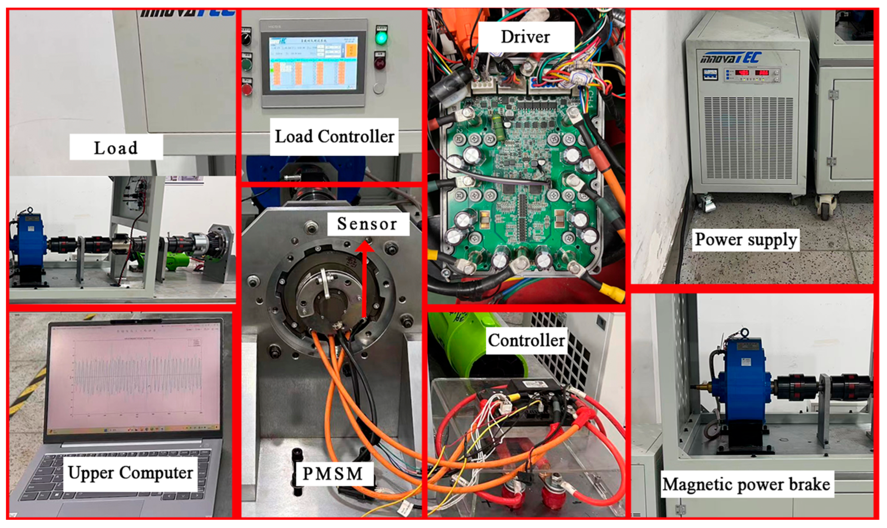
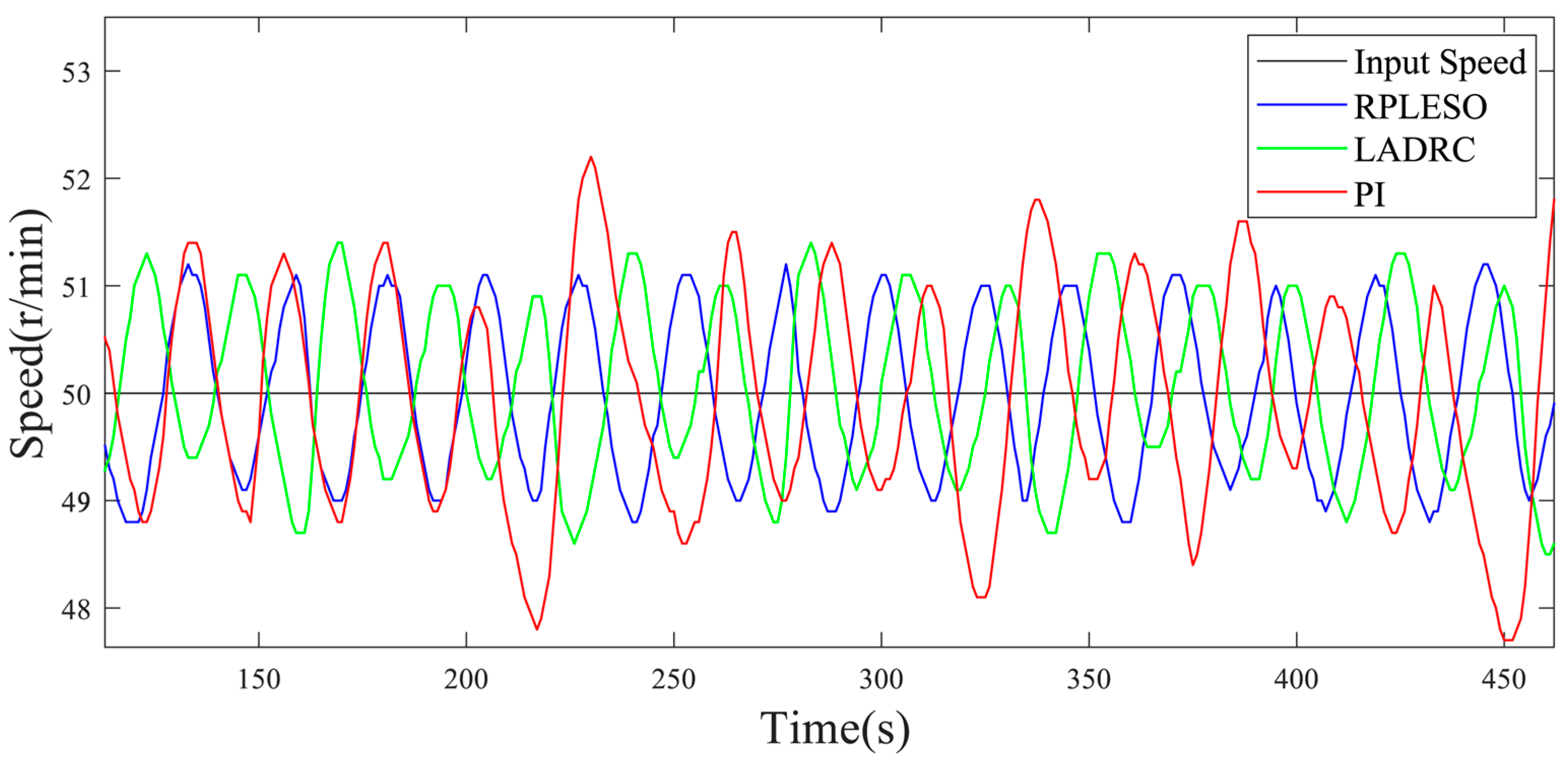
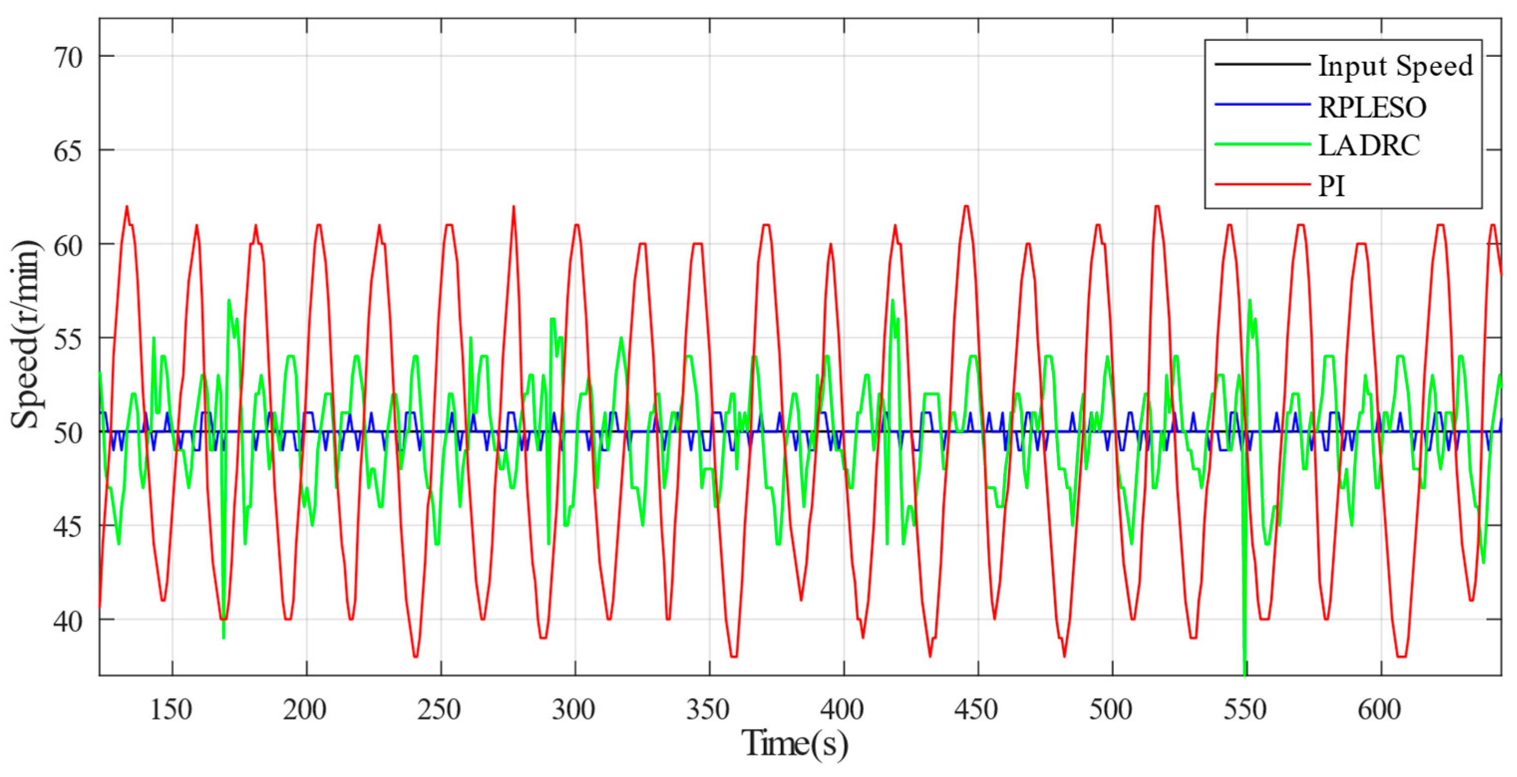
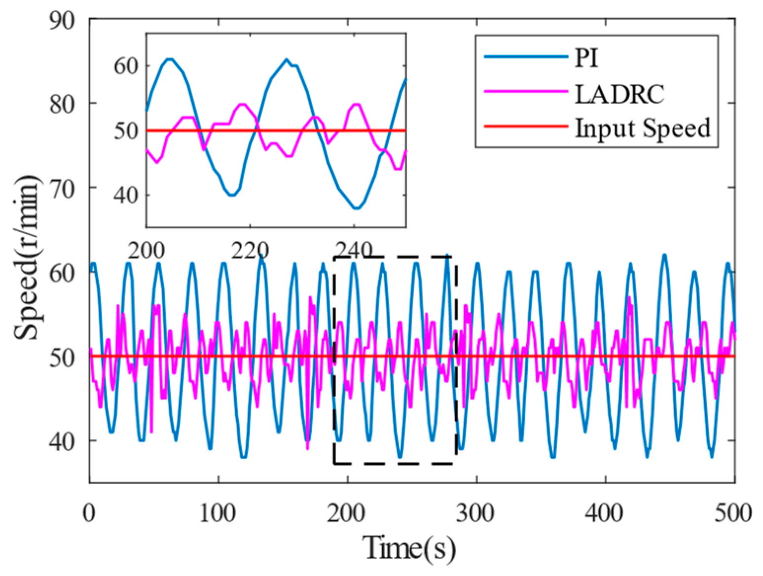
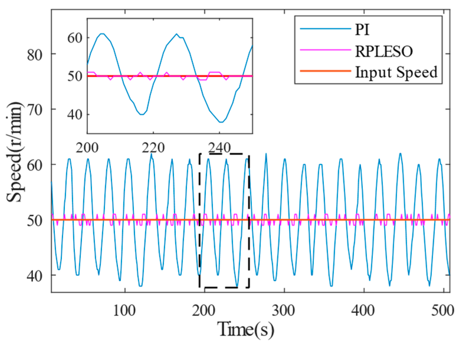
In order to further prove the practicality of the improved active disturbance rejection control algorithm based on the proposed RPLESO in engineering practice, a set of back-to-back experimental platforms composed of a CDC-S130B motor and magnetic powder dynamometer is built, with LKS32MCO80R8T8 as its main controller, as shown in Figure 10. When the reference speed of the test platform is 50 r/min, the steady-state speed control accuracy of the three control strategies under no load and a 40 N·m load is obtained, as shown in Figure 11 and Figure 12, respectively. The data obtained from the experiments are exported to an Excel file via the host computer. The data file is then imported into MATLAB for plotting. By adjusting the size and local zoom of the data waveforms under different experimental conditions in each image, the vector graphics are exported. MATLAB’s data statistics functions are used to compare the motor speed waveforms and the stability under load disturbances under different experimental conditions.

We calculate the speed fluctuation error under the three control algorithms in Figure 11 and Figure 12 based on the standard deviation in Formula (19), as shown in

Table 5. Standard deviation of speed fluctuation in three control modes.

Project	RPLESO	LADRC	PI
Unload	7.44	7.79	9.42
Load	0.55	2.91	7.44

.

$$s=\sqrt{\frac{{(x_1-x)}^2+{(x_2-x)}^2+\cdot \cdot \cdot {(x_n-x)}^2}{n-1}}$$

(19)

The speed fluctuation of the RPLESO is comparable to that of LADRC when the motor is unloaded but significantly smaller than those of the other two control methods when loaded.

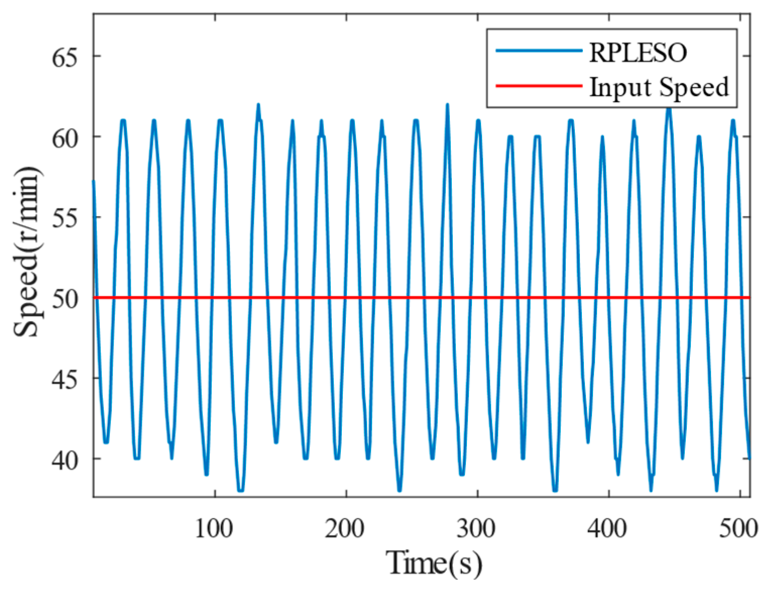
In order to test the robustness of the proposed control strategy and the traditional LADRC and PI control under a disturbance, as well as the precision in the observing the speed, the reference speed is set at 50 r/min, and the speed fluctuations under no load and a 40 N·m load are, respectively, tested. As shown in Figure 12 and Figure 13, the active disturbance rejection control based on the RPLESO has strong robustness to disturbances, and the speed fluctuation is the smallest under no load and a disturbance. Therefore, compared with traditional control, the active disturbance rejection control optimized in this paper has good speed observation accuracy and tracking performance and stronger robustness.

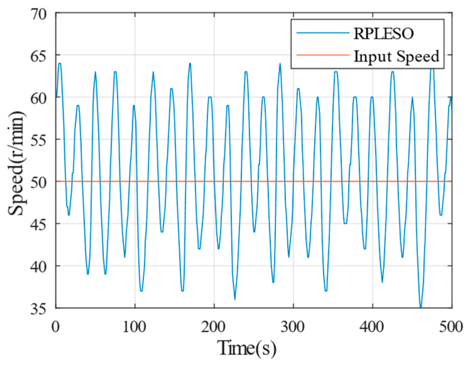
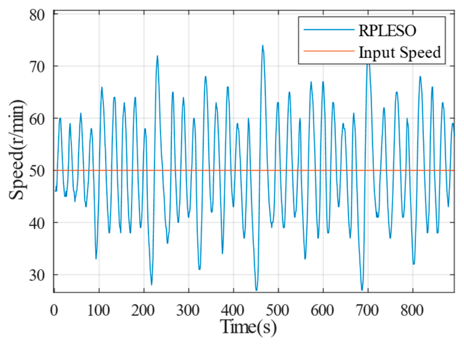
We compare the speed on the motor side with the output speed after adding a reducer to the motor, as shown in Figure 14, Figure 15, Figure 16, Figure 17, Figure 18, Figure 19, Figure 20, Figure 21, Figure 22 and Figure 23. Although the low-speed torque is increased when adding a reducer on the outside of the motor, the speed fluctuation also increases compared to the previous case, which leads to vibration in non-road vehicles at low speeds. To address this issue, we will consider improving it by reducing the order of the linear ADRC and adding digital filtering algorithms in the feedback loop.

5. Conclusions

This paper applies LADRC in a PMSM double closed loop control system, proposes an improved LADRC control based on order-reduced parallel linear active disturbance rejection control and provides the design of a velocity loop LADRC controller and the parameters of the current loop PI controller. The simulation analysis and experimental verification show that

• The LADRC speed loop controller based on the RPLSEO can improve the steady-state speed precision of the system and effectively solve the problem of vehicle jitter at low speeds;
• The improved LADRC controller can obtain better observation performance than the traditional LADRC under the condition of an actual bandwidth limitation, thus reducing the application cost of the control system and having more practical application value;
• The algorithm proposed in this paper reduces the adjustable parameters of the system speed controller to four, improves the tunability of the parameters, makes the system more robust and can reach stability faster after being disturbed.