Ultra-Short-Term Wind Power Prediction Based on the ZS-DT-PatchTST Combined Model

Abstract

When using point-by-point data input with former series models for wind power prediction, the prediction accuracy decreases due to data distribution shifts and the inability to extract local information. To address these issues, this paper proposes an ultra-short-term wind power prediction model based on the Z-score (ZS), Dish-TS (DT), and Patch time series Transformer (PatchTST). Firstly, to reduce the impact of data distribution shift on prediction accuracy, ZS standardization is applied to both training and testing datasets. Additionally, the DT algorithm, which can self-learn the mean and variance, is introduced for window data standardization. Secondly, the PatchTST model is employed to convert point input data into local-level input data. Feature extraction is then performed using the multi-head attention mechanism in the Encoder layer and a feed-forward network composed of one-dimensional convolution to obtain the prediction results. These results are subsequently de-standardized using DT and ZS to restore the original data amplitude. Finally, experimental analysis is conducted, comparing the proposed ZS-DT-PatchTST model with various prediction models. The proposed model achieves the highest prediction accuracy, with a mean absolute error of 5.95 MW, a mean squared error of 10.89 MW, and a coefficient of determination of 97.38%.

1. Introduction

As the proportion of wind power in global electricity generation increases, wind power prediction has become crucial to fully utilize wind energy and ensure the safe and stable operation of the power grid. Wind power prediction can be categorized into long-term [1,2,3], medium-term [4,5], short-term [6,7], and ultra-short-term predictions [8,9,10]. Long-term and medium-term predictions have lower accuracy requirements and are less studied [11]. Short-term prediction refers to forecasting wind power generation within three days, while ultra-short-term prediction focuses on forecasting wind power generation within the next 4 h [12]. Ultra-short-term wind power prediction enables frequency regulation of wind turbines, optimization of spinning reserve capacity, and economic load distribution, making it a hot topic in the wind power industry.

With the advent of deep learning, more and more time series prediction models have been applied to wind power prediction. For instance, reference [13] proposed a novel long short-term memory (LSTM) architecture based on backpropagation to predict the ultra-short-term wind power in an adaptive way. In [14], convolutional neural networks (CNN) and LSTM are combined to predict wind power and weighted using adaptive optimization to improve the computational efficiency, and then the adaptive moment estimation (Adam) optimization algorithm is used to minimize the loss and improve the prediction accuracy of the model. In [15], it was proposed to use an autoencoder to extract potential features from wind speed data and then predict them by LSTM, which improved the accuracy by 39% compared to the traditional method. Subsequently, researchers simplified the structure of the LSTM to reduce the risk of gradient vanishing, and the gated recurrent unit (GRU) model emerged and was applied to the field of wind power prediction. For example, Ref. [16] proposes to use complete ensemble empirical mode decomposition with adaptive noise (CEEMDAN) to decompose multiple subsequences and then use the GRU model to predict each subsequence, and the prediction results of each sub-sequence are superimposed together to obtain the final wind power prediction results, which improves the prediction accuracy of the model. However, LSTM and GRU models are weak in parallel computation and interpretability, which often leads to lower model prediction accuracy when facing complex and variable data. To address these issues, time series prediction models based on Transformers have emerged [17,18,19]. Transformer models utilize attention mechanisms for parallel computation, establishing correlations between data points, extracting features, improving the interpretability of the model, and reducing the risk of gradient explosion.

However, due to the computational complexity of the attention mechanism, models like Informer and Autoformer have been developed to simplify this complexity and have been widely used in time series prediction. For example, the MSRN-Informer model introduced in [20] incorporates a multi-scale structure to extract data features at different scales and employs a residual network to reduce data loss. In [21], the Informer model is applied to predict parameters in various scenarios. The Autoformer-CSA model proposed in [22] introduces a channel–spatial attention module (CSAM) to replace the feed-forward network of the Autoformer, improving prediction accuracy. Additionally, Ref. [23] presents a combination method based on multisource information fusion (MIF) and Autoformer models, achieving feature-level and data-level information fusion. However, with the in-depth study of the former series model, reference [24] found that the former series model with the above point-level inputs could not extract the local information and keep the channel independence, which led to the reduced prediction accuracy of the former series model. For this reason, a Patch time series Transformer (PatchTST) model is proposed, which adopts a channel-independent Patch structure to divide the time series data into a number of localities, establish local correlations, and carry out local information feature extraction while maintaining channel independence, and has been widely used. For example, the literature [25] uses the PatchTST model to convert point-level inputs into local-level inputs through Patch. It is combined with the convolutional network to extract deeper local information, which improves the prediction accuracy of the model, and the literature [26] verifies that the PatchTST model still has a certain degree of accuracy in the field of forecasting.

For time series data often exhibit distribution shifts, which can reduce the accuracy of time series prediction models. This distribution shift can occur between the training set and the test set, as well as between different windows of data. To address the distribution shift between the training set and the test set, the Z-score (ZS) method is used to calculate the mean and variance of the observed data for standardization and de-standardization. For example, Ref. [27] pointed out that the ZS algorithm can standardize the data with the problem of shift and reduce the distribution difference; Ref. [28] used the ZS algorithm for standardization in order to reduce the distribution shift and reduce the operation complexity, which helped the model to improve the accuracy by 0.729%. For the problem of distribution shift between different windows, the reversible instance normalization(RevIN) model was first proposed in [29], which normalizes each window to reduce the distribution difference between windows; subsequently, researchers started to combine the RevIN(RV) model with timing prediction models, dedicated to solving the impact of the window distribution shift problem on timing prediction models, such as the practical application of the NSTransformer model [30] and iTransformer model [31]. With the in-depth study of the window distribution shift problem, a more advantageous Dish-TS (DT) model [32] has emerged, which is able to adaptively learn the mean and variance required for standardization and de-standardization, which further reduces the impact of the window distribution shift problem on the prediction accuracy of the model compared to the RV. Similarly, the DT model also has the ability to be combined with the time-series prediction model to help improve its prediction accuracy. For example, Ref. [33] combines DT with GRU, learns mean and variance through the DT model for standardization, and uses the GRU model to obtain prediction results; the prediction results are then de-standardized. This self-learning standardization and de-standardization method reduces the impact of window distribution shift on the GRU model and improves its prediction accuracy.

In summary, the point–input former series models experience a decline in prediction accuracy for wind power due to distribution shifts in wind power data and the inability to extract local information of wind power data. To address these issues, this paper proposes an ultra-short-term wind power prediction model based on ZS-DT-PatchTST. The main contributions of this paper are as follows: firstly, through data analysis, we verify the existence of wind power data with distribution shift phenomenon; second, a combined processing method of ZS-DT is proposed, which is dedicated to solving the impact of the wind power data distribution shift problem on the prediction accuracy of the model; third, the ZS-DT is combined with the PatchTST model to complete the prediction work, and to improve the defects of the former series model with point-level inputs that are unable to extract the local information of the wind power data.

The structure of the paper is as follows: In Section 2, the distribution shift in wind power data and the correlation between data points are analyzed. In Section 3, the ZS-DT-PatchTST model is introduced. ZS and DT are employed to reduce the impact of distribution shifts in wind power data on prediction accuracy. The PatchTST model is used to divide the wind power data into multiple local Patches, and a multi-head attention mechanism is applied to establish local correlations and extract features. In Section 4, simulation experiments are conducted for analysis. A brief conclusion is provided in Section 5.

2. Analysis of Wind Power Data Characteristics

In this study, we use a publicly available dataset from a wind power plant with an installed capacity of 200 MW. The data were collected at 15 min intervals, resulting in a total of 34,071 data points. The dataset consists of 12 channels (features) arranged in numerical order from 1 to 12, as shown in

Table 1. Channel definitions.

Channel	Feature Name
1	Wind speed at height of 10 m (m/s)
2	Wind direction at height of 10 m (°)
3	Wind speed at height of 30 m (m/s)
4	Wind direction at height of 30 m (°)
5	Wind speed at height of 50 m (m/s)
6	Wind direction at height of 50 m (°)
7	Wind speed at the height of wheel hub (m/s)
8	Wind direction at the height of wheel hub (°)
9	Air temperature (°C)
10	Atmosphere pressure (hpa)
11	Relative humidity (%)
12	Wind Power (MW)

.

2.1. Analysis of Distribution Shift in Wind Power Data

In wind power prediction, the statistical properties, such as the mean and variance of each channel, change over time, resulting in a distribution shift. This phenomenon often leads to a decrease in the accuracy of model predictions [29,32]. In this paper, we take the actual wind power data from channel 12 as an example and use Equation (1) to calculate its mean and variance [34].

$$\left\{\begin{array}{l}{m}_{\beta }={\displaystyle \frac{{\displaystyle \sum _{i=1}^n{x}_i}}{n}}\\ v_{\beta }={\displaystyle \frac{{\displaystyle \sum _{i=1}^n{\left(x_i-m_{\beta }\right)}^2}}{n}}\end{array}\right.$$

(1)

where x_i represents the original channel data, β is the channel number, n denotes the total number of data points, m_β is the mean of channel β, and v_β is the variance of channel β.

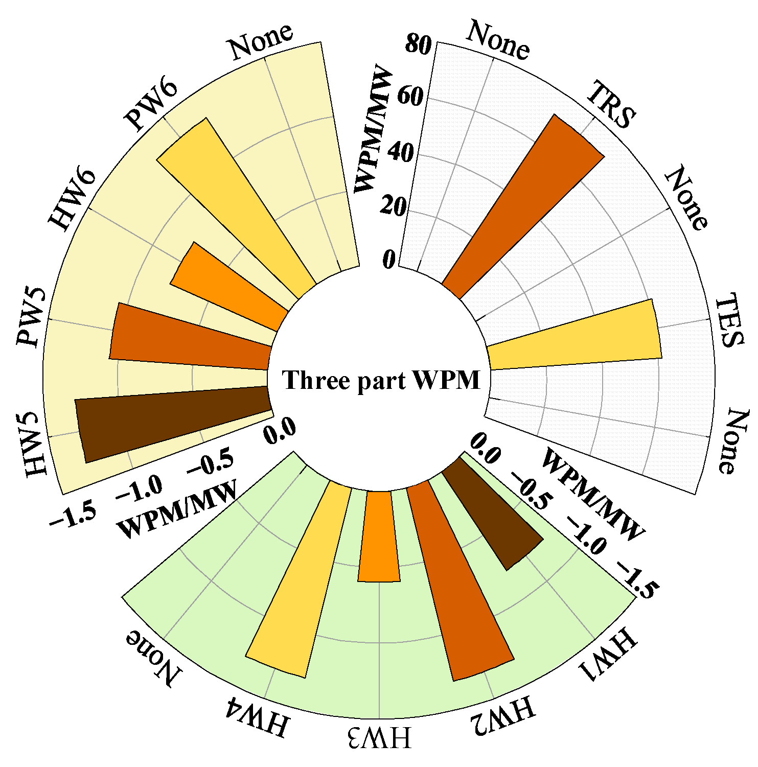
2.1.1. Mean Analysis

Calculating the mean plays a significant role in analyzing whether the data distribution has shifted [35]. The mean values for the training set, test set, historical window, and prediction window are calculated using Equation (1). Some of the results are shown in Figure 1.

In Figure 1, WPM represents the wind power mean. In the blue area, TRS stands for the training set, and TES stands for the test set. The mean calculation results for TRS and TES in this area differ by about 10. In the green area, HW1–HW4 represent the means of four different historical windows extracted using a sliding window approach, and it is evident that there are significant differences in the means of these four historical windows. In the yellow area, HW5 is a historical window extracted using a sliding window, and PW5 represents the prediction window corresponding to HW5. It can be seen that there is a significant difference in the means between HW5 and PW5, as well as between HW6 and PW6. This indicates that there are differences in the means of the training set, test set, historical windows, and prediction windows.

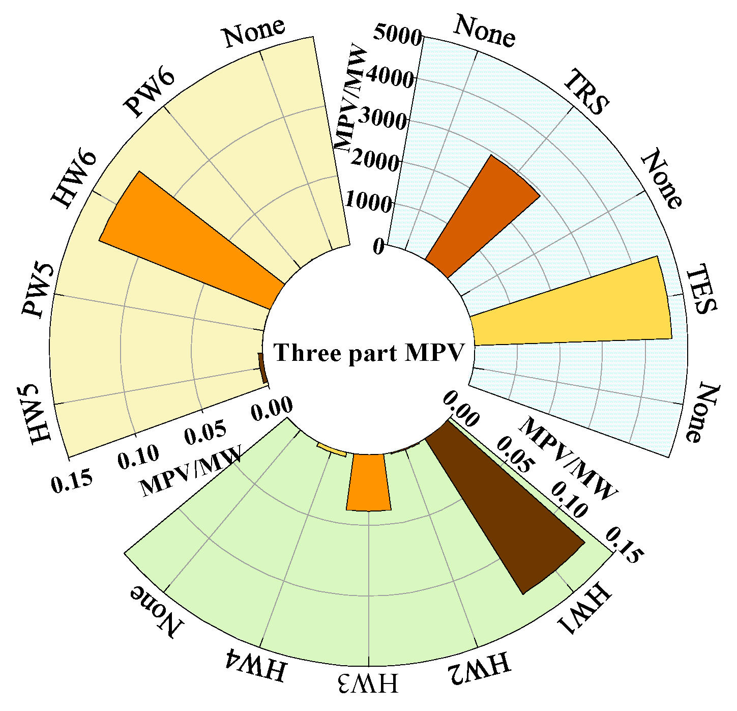
2.1.2. Variance Analysis

The variances for the training set, test set, historical window, and prediction window are calculated using Equation (1). Some of the results are shown in Figure 2.

In Figure 2, MPV represents the wind power variance. In the blue area, the variance calculation results for the training set (TRS) and the test set (TES) show a difference of approximately 2000. In the green area, the variances for HW1, HW2, HW3, and HW4 are all different. In the yellow area, the variances for PW5 and PW6 are close to zero, while there are significant differences between the variances of HW5 and PW5, as well as HW6 and PW6.

From the above analysis, it can be concluded that there are significant differences in the means and variances between the training set and test set, among historical windows, and between historical windows and prediction windows, indicating the presence of a distribution shift.

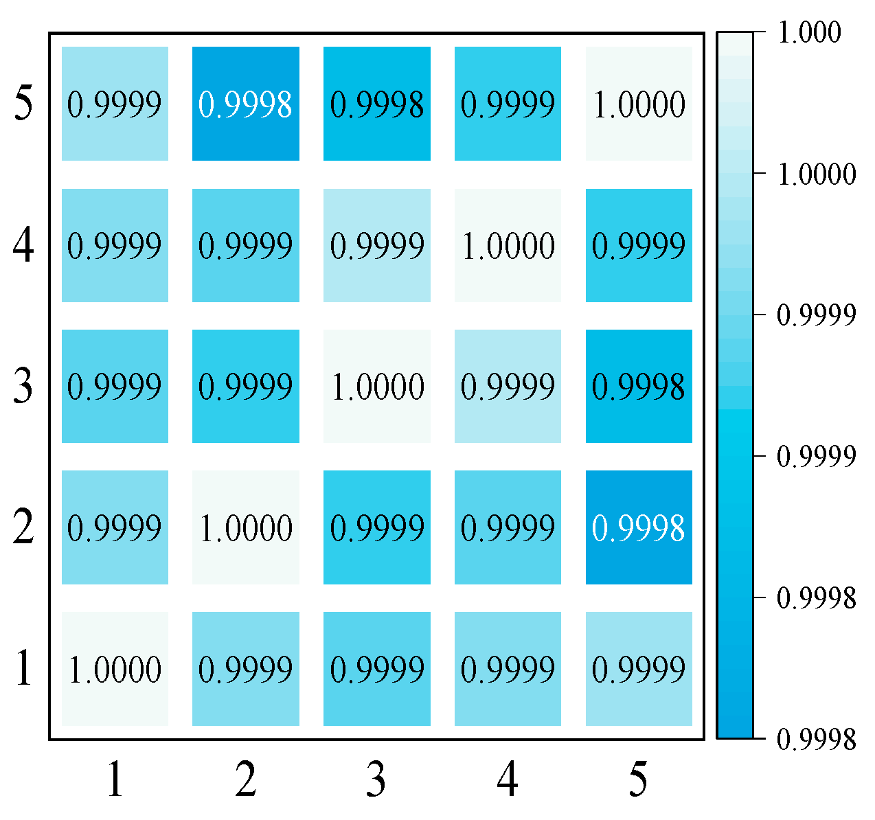
2.2. Analysis of Data Point Correlation in Wind Power Data

Five data points from the dataset are selected, specifically from 1 January, 00:00, to 1 January, 01:00. The correlations between these data points are calculated using Equation (2) [36,37], and a heatmap is generated, as shown in Figure 3.

$$r_{x,y}={\displaystyle \frac{{\displaystyle {\sum }_{i=1}^N(x_i-\overline{x})(y_i-\overline{y})}}{\sqrt{{\displaystyle {\sum }_{i=1}^N{(x_i-\overline{x})}^2}}\times \sqrt{{\displaystyle {\sum }_{i=1}^N{(y_i-\overline{y})}^2}}}}$$

(2)

where r is the Pearson correlation coefficient, x_i is the ith observation of the variable x, $\overline{x}$ is the mean of the variable x, y_i is the ith observation of the variable y, $\overline{y}$ is the mean of the variable y, and N represents the total number of observations contained in the variables x and y.

In Figure 3, the horizontal and vertical coordinates 1–5 represent five different data points. Each square in the figure represents the correlation between data points. From Figure 3, it can be seen that the correlation between each pair of data points is greater than 0.99. This indicates that, within a local range, each data point has a significant correlation with its surrounding data points; exploring local correlations may be of great significance.

3. Prediction Model Based on ZS-DT-PatchTST

When using the point level input of the former series model for wind power prediction, there are the following problems: Problem 1 is that there is a distribution shift phenomenon in the wind power data. In Problem 2, time series forecasting aims to understand the correlation between data in each different time step. However, a single time step does not have semantic meaning like a word in a sentence, so extracting local semantic information is essential in analyzing their connections. However, the point level input of the former series model cannot integrate related wind power data points into multiple local areas and explore the correlation between local areas. Problem 3 is that the former series models with point-level inputs cannot maintain channel independence, which can lead to a decrease in model prediction accuracy [24,32]. In response to the above issues, this article proposes an ultra-short-term wind power prediction model based on the ZS-DT-PatchTST model, as shown in Figure 4.

In Figure 4, firstly, ZS standardization is performed on the original wind power data (WPD), and the history window (HW) is obtained by adopting the most commonly used method of sliding window extraction in time series prediction, and the HW is put into the DT module, so as to reduce the impact of the wind power data distribution bias on the prediction accuracy through the ZS-DT model. Secondly, the HW after DT is put into the channel-independent Patch module, which is divided into a number of localities while maintaining channel independence, and the divided localities are put into the Encoder layer to extract local information from the wind power data, and then the output of the Encoder is put into the Linear layer to obtain the standardized prediction result, which improves the defects of the point-level input model that cannot maintain channel independence and extract local information. Finally, the output of the Linear layer is put into the DT de-standardization (DT-De) and ZS de-standardization (ZS-De) modules successively for de-standardization to obtain the final prediction results. In this paper, the workflow of each module of the ZS-DT-PatchTST architecture is described in detail in Section 3.1, Section 3.2 and Section 3.5, taking the WPD in Section 2 as an example.

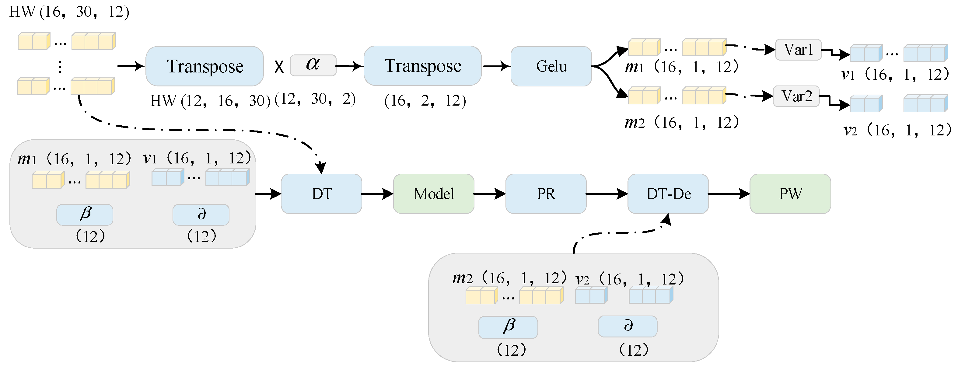
3.1. ZS Module

The ZS standardization method is used to address the distribution shift problem between the training set and the test set of WPD. To ensure that the statistical characteristics of the training data and test data are consistent, the mean and variance of each channel in the training set are calculated using Equation (1). Then, these calculated mean and variance values are used in Equation (3) to perform ZS standardization on each channel of both the training set and the test set.

$$Z_{\beta }={\displaystyle \frac{(x_i-m_{\beta })}{\sqrt{v_{\beta }}}}$$

(3)

where x_i represents the original channel value, m_β represents the channel mean, and v_β represents the channel standard deviation.

The de-standardization formula is shown in Equation (4).

$$T_{\beta }=Z_{\beta }\times \sqrt{v_{\beta }}+m_{\beta }$$

(4)

where Z_β represents the predicted channel value, v_β represents the channel standard deviation, and m_β represents the mean of the original input channel data.

3.2. DT Module

After solving the distributional bias between the WPD training and test sets using ZS, samples were extracted using the sliding window method to obtain the HW. Sixteen different HWs were loaded into the model at a time during training to calculate the loss and update the internal weights of the model. To address the distribution shift problem between different windows, the DT model was employed. This model can self-learn the mean and variance needed for standardization and de-standardization [32], thereby improving prediction accuracy. The DT model architecture is shown in Figure 5.

In Figure 5, HW represents the history window of the input model with the dimension (16, 30, 12), which means 16 different history windows, each with 30 time steps and 12 features. Firstly, three learnable weights are initialized: an α matrix with dimensions (12, 30, 2), a one-dimensional sequence β with dimension (12), and a one-dimensional sequence ∂ with dimension (12). HW is then transposed to (12, 16, 30) and multiplied with α. After transposing the result of multiplying the two to (16, 2, 12), it is put into the activation function Gelu to perform the nonlinear transformation, and the result after Gelu is divided into m₁ and m₂; m₁ and m₂ are put into Var1 and Var2 to find the variance, respectively, and obtain ν₁ and ν₂, where m₁, m₂, ν₁, ν₂ dimensions are (16, 1, 12). Secondly, m₁, ν₁, β, ∂, and HW are put into DT standardization operation for each HW using Equation (5). Finally, it is put into the PatchTST model for prediction to obtain the model output PR, and then m₂, ν₂, β, ∂, and PR are put into the DT-De de-standardization operation using Equation (6). The whole process needs to pay attention to two points: firstly, Var1 and Var2 to find the variance algorithm given in Equation (1); secondly, the weight dimensions are based on the above, and the dimensions correspond automatically through the broadcasting mechanism when defining the weights for the calculation using PyTorch-gpu 2.1.0.

$$\left\{\begin{array}{l}{x}_1={\displaystyle \frac{\left(x-m_1\right)}{\sqrt{v_1}}}\\ z=x_1\times \beta +\partial \end{array}\right.$$

(5)

where x is the model input HW, m₁ is the mean of the input sequence, ν₁ is the variance of the input sequence, β is the scaling factor, and ∂ is the translation factor.

$$x_i=\left((x_o-\partial )/\beta \right)\times \sqrt{v_2}+m_2$$

(6)

where x_o is the model output results PR, ν₂ is the variance of the output sequence, and m₂ is the mean of the output sequence.

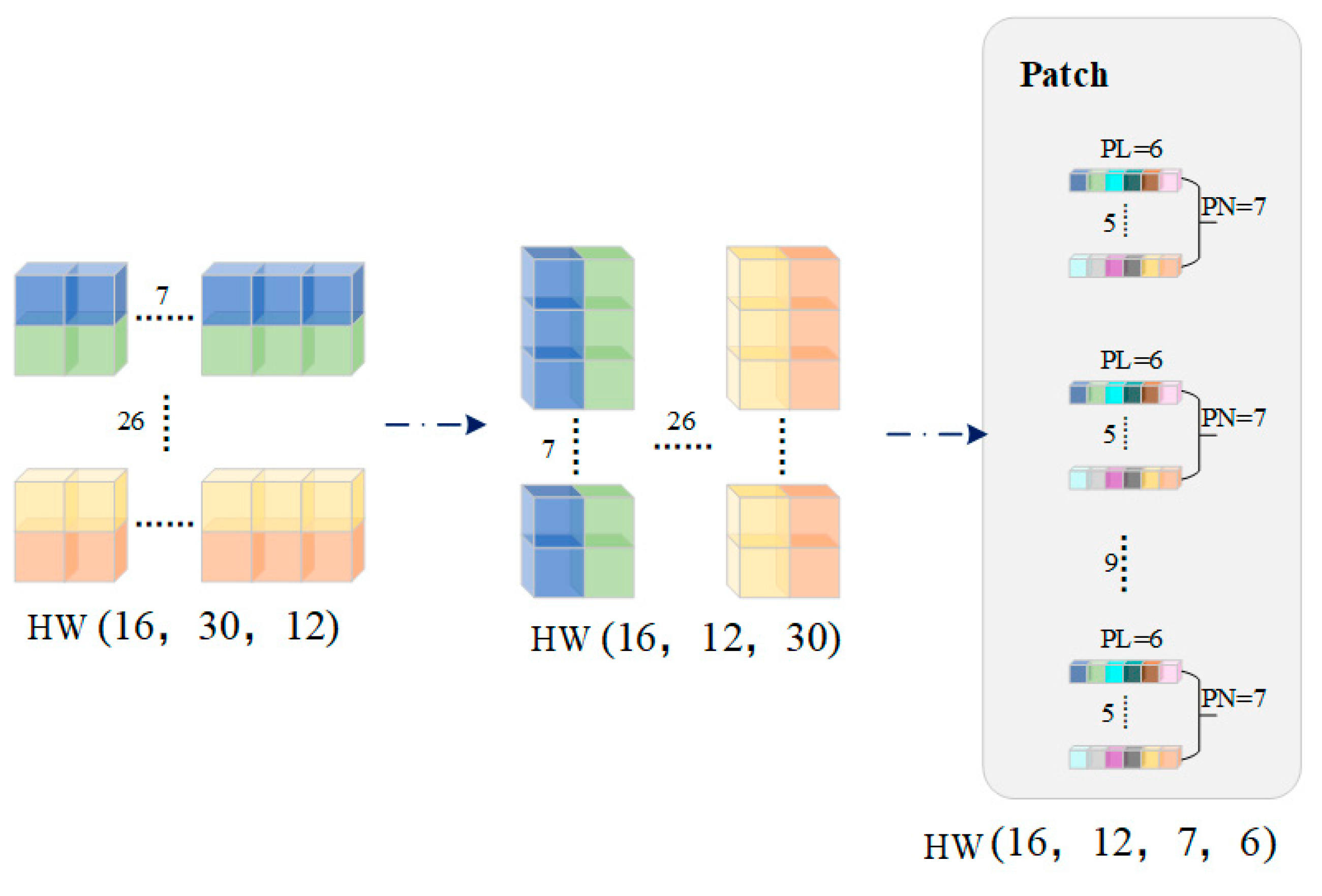
3.3. Patch Module

When using the former series model with point-level inputs for prediction, it is not possible to keep the channels independent and extract the local information, and this problem degrades the accuracy of the former series model [24]. To solve this problem, the DT-processed HW in Section 3.2 is divided into several localizations using a channel-independent Patch structure, the architecture of which is shown in Figure 6.

In Figure 6, the DT standardization processed HW is transposed to (16, 12, 30). Then, PL is set to 6 and S to 4, according to Equation (7); the last dimension is split to produce an output of (16,12, 7, 6), where 7 represents the number of Patches, and 6 represents the number of data points in each Patch. This method retains channel independence while integrating adjacent correlated data sampling points into one Patch.

$$PN={\displaystyle \frac{\left(T-PL\right)}{S}}+1$$

(7)

where T is the length of the time steps, PL is the length of the Patch time steps (Patch_len), S is the stride, and 1 is a constant.

3.4. Embedding and Encoder

The output of HW after passing the Patch is put into the Embedding layer and Encoder layer to extract the local information of wind power data, where the Encoder adopts the Encoder architecture of the Transformer model, which is shown in Figure 7.

In Figure 7, the output result of Patch module (16, 12, 7, 6) is changed to (16 × 12, 7, 6) and then put into Embedding layer, which outputs a matrix with dimension (16 × 12, 7, 512), and the matrix is passed through the three linear layers to obtain Q, K, V, respectively, and then through the multi-attention mechanism Equation (8), the local correlation is established and local information is extracted. After this, through the Add&Norm layer, where Add is the output of the multi-attention mechanism plus the Embedding output, and then put into the Norm layer for layer normalization operation, the output dimension is still (16 × 12, 7, 512). After completing the above operation, it is put into the Feed Forward layer, and the layer architecture is Conv1d-Gelu-Conv1d; firstly, the output result of the previous layer Add&Norm is put into the first one-dimensional convolution (Conv1d) for depth extraction of features, and the dimensionality is expanded to (16 × 12, 7, 2048); secondly, it is put into the Gelu for nonlinear transformation; finally, it is put into the second Conv1d transformation dimension of (16 × 12, 7, 512). After completing the above operations, it is put into the Add&Norm layer to obtain the output result of the Encoder layer. In this paper, the Encoder layer building process needs to be noted that, first, the linear layer output dimension of all modules should be 512 to ensure that the Encoder input and output dimensions are the same; second, the Encoder layer in the linear layer, the one-dimensional convolutional layer, the Norm layer in the model building process can be called directly through Pytorch.

$$\left\{\begin{array}{l}Scor{e}_{(\omega )}=\mathrm{soft}\max \left({\displaystyle \frac{Q\times K^T}{\sqrt{d_k}}}\right)\\ C=Scor{e}_{(\omega )}\times V\end{array}\right.$$

(8)

where Q represents the query matrix, K represents the key matrix, V represents the value matrix, and $\sqrt{d_k}$ is a scaling factor to limit the range of the attention weights.

3.5. DT-Std Layer and ZS-De-Std Layer

The output of the Encoder is fed into a Linear layer. Finally, the prediction results obtained from the Linear layer undergo de-standardization operations sequentially via DT-De and ZS-De, restoring the data to its original scale. Note that the DT-De and ZS-De denormalization methods are described in detail in Section 3.1 and Section 3.2.

4. Experimental Analysis

During the experiment, two datasets with different acquisition frequencies were selected to analyze the performance of the model on different time scales. Wind power dataset 1 comes from the dataset used in Section 2 of this paper, with an acquisition frequency of 15 min, 12 column variables, 24,447 samples in the training set, and 1152 samples in the test set; wind power dataset 2 comes from the dataset of a wind farm with an installed capacity of 100 MW, and the data are collected every 5 min data collection, a total of 21,100 data points, one column variable, 14,737 training set samples, 702 test set samples. The calculations in this paper were carried out on the PyCharm platform based on AMD Ryzen 7 5800H processor (Ryzen, San Jose, CA, USA), 16 GB RAM, NVIDIA GeForce RTX 3050 Ti (NVIDIA, Santa Clara, CA, USA), and the runtime environment is PyTorch-gpu 2.1.0 based on Python 3.9.7.

4.1. Evaluation Metrics

The prediction results were evaluated using root mean squared error (RMSE), mean absolute error (MAE), and the coefficient of determination (R²). The formula for RMSE is given by Equation (9):

$$\mathrm{RMSE}=\sqrt{{\displaystyle \frac{1}{n}}{\displaystyle \sum _{i=1}^n{\left(Y_i-{\widehat{Y}}_i\right)}^2}}$$

(9)

where Y_i is the actual value, Ŷ_i is the predicted value, and n is the number of test samples.

The formula for MAE is given by Equation (10):

$$\mathrm{MAE}={\displaystyle \frac{1}{n}}{\displaystyle \sum _{i=1}^n\left|Y_i-{\widehat{Y}}_i\right|}$$

(10)

The R² is used to evaluate the performance of the regression model. R² represents the proportion of variance between the predicted and observed values. The closer the R² value is to 1, the higher the degree of fit. The formula for the R² is given by Equation (11):

$$R^2=1-{\displaystyle \frac{{\displaystyle \sum _{i=1}^n{\left(Y_i-\widehat{Y}\right)}^2}}{{\displaystyle \sum _{i=1}^n{\left(Y_i-{\overline{Y}}_i\right)}^2}}}$$

(11)

4.2. Hyperparametric Analysis

Analysis of hyperparameter configurations during experiments helps models improve prediction accuracy [38,39]. The model setup hyperparameters in this paper are shown in

Table 2. Model hyperparameter configuration.

Hyperparameter Name	Parameter Setting
Batch_size	16
Train_epochs	30
D_model	512
H_heads	8
Encoder_layers	3
Patch_len	6
Stride	4
Dropout	0.05
Learning_rate	Adaptive Optimization

.

In Table 2, the three most important hyperparameters for model training in this paper are namely Batch_size, Encoder_layers, and Patch_len. Batch_size decides the number of samples to be loaded at one time, which plays an important role in calculating the loss and training model; Encoder_layers decides how many Encoder layers are stacked, which plays a key role in extracting the historical features; Patch_len determines how many data points are in a locality and is important for exploring local correlations. Wind power dataset 1 is selected to evaluate the prediction accuracy of the test set as well as the average training time per round, and three hyperparameter ranges are determined, as shown in

Table 3. Hyperparameter Batch_size.

Parameter Values	MAE/MW	RMSE/MW	Time/s
8	6.69	11.74	506.75
12	6.60	11.86	483.75
16	5.95	10.89	465.03
20	6.67	11.79	457.85
24	6.49	11.69	717.24

,

Table 4. Hyperparameters Encoder_layers.

Parameter Values	MAE/MW	RMSE/MW	Time/s
1	6.59	11.66	162.14
2	7.02	11.89	317.34
3	5.95	10.89	465.03
4	6.23	11.35	1547.77

and

Table 5. Hyperparameters PL.

Parameter Values	MAE/MW	RMSE/MW	Time/s
4	6.92	11.74	465.32
5	6.65	11.67	416.81
6	5.95	10.89	465.03
7	6.66	11.65	308.79
8	6.28	11.58	257.45

.

4.2.1. Batch_Size Hyperparameter Analysis

The rest of the hyperparameter values are kept unchanged, and the memory is considered to set the Batch_size to 8, 12, 16, 20, and 24, respectively, as shown in Table 3.

In Table 3, when the number of Batch_size is 16, compared with Batch_size of 8, the MAE and RMSE are reduced by 0.74 MW and 0.85 MW, respectively, and the average training time per round is reduced by 41.72 s; compared with Batch_size of 12, the MAE and RMSE are reduced by 0.65 MW and 0.97 MW, respectively, and the average training time per round is reduced by 18.72 s; compared with Batch_size of 20, MAE and RMSE are reduced by 0.72 MW, 0.90 MW, and the average training time per round is increased by 7.18 s; compared with Batch_size of 24, MAE and RMSE are reduced by 0.54 MW, 0.80 MW, and the average time training per round is reduced by 252.21 s. To sum up the data, the model prediction accuracy is higher when Batch_size is 16, and when bacth_size is 24, the model prediction accuracy starts to decrease, and the time increases instead, so the Batch_size of 12–20 is a reasonable range.

4.2.2. Encoder_Layers Hyperparameter Analysis

The rest of the hyperparameters are kept unchanged, and the Encoder_layers are set to 1, 2, 3, and 4, respectively, as shown in Table 4.

In Table 4, when Encoder_layers is 3, compared to when Encoder_layers is 1, MAE and RMSE are reduced by 0.64 MW and 0.77 MW, respectively, and the average training time per round is increased by 302.89 s; compared to when Encoder_layers is 2, MAE and RMSE are reduced by 1.07 MW, respectively, 1.00 MW, and the average training time per round increased by 147.69 s; compared to when Encoder_layers is 4, the MAE and RMSE decreased by 0.28 MW and 0.46 MW, respectively, and the average training time per round decreased by 1082.74 s. When summing up the above data, affected by the model prediction accuracy and the training speed, we ultimately chose Encoder_layers of 3.

4.2.3. Patch_Len Hyperparameter Analysis

The rest of the hyperparameters are kept unchanged, and the Patch_len is set to 4, 5, 6, 7, and 8, as shown in Table 5.

In Table 5, when Patch_len is 6, compared to when Patch_len is 4, MAE and RMSE decreased by 0.97 MW and 0.85 MW, respectively, and the average training time per round decreased by 0.29 s; compared to when Patch_len is 5, MAE and RMSE decreased by 0.70 MW and 0.78 MW, respectively, and the average training time per round increased by 48.22 s; compared to when Patch_len is 7, MAE and RMSE decreased by 0.71 MW and 0.76 MW, respectively, and the average training time increased by 156.24 s; compared to when Patch_len is 8, MAE and RMSE decreased by 0.33 MW and 0.69 MW, respectively, and the average training time increased by 207.58 s. In summary, the difference in the average training time between Patch_len 4–6 is small, and if there is a strict requirement of the training time of mode, you can set the Patch_len to 7. In this paper, considering the accuracy of the model, we finally choose the Patch_len to be 6.

4.3. Experimental Results and Analysis

Error analyses are performed on the test set prediction results for wind power dataset 1 and wind power dataset 2 with collection frequency of 15 min and 5 min. The chapters are arranged as follows: In Section 4.3.1 and Section 4.3.2, the wind power dataset 1, with data collected every 15 min, is used as the basis to verify that the model prediction accuracy is improved after the ZS-DT module handles the problem of wind power data distribution bias. In Section 4.3.3, based on the wind power dataset 1 with data collected every 15 min, the proposed model in this paper is compared and analyzed with common time series prediction models to verify that the model in this paper has certain advantages. In Section 4.3.4, based on the wind power dataset 2 with data collected every 5 min, the model proposed in this paper is compared with the common time series prediction models to verify that the model proposed in this paper still has high prediction accuracy for different time scales. For wind power dataset 1, in order to present a clearer comparison of the prediction curves of different models, 600 data points were extracted to plot model comparison curves to facilitate observation of the fit.

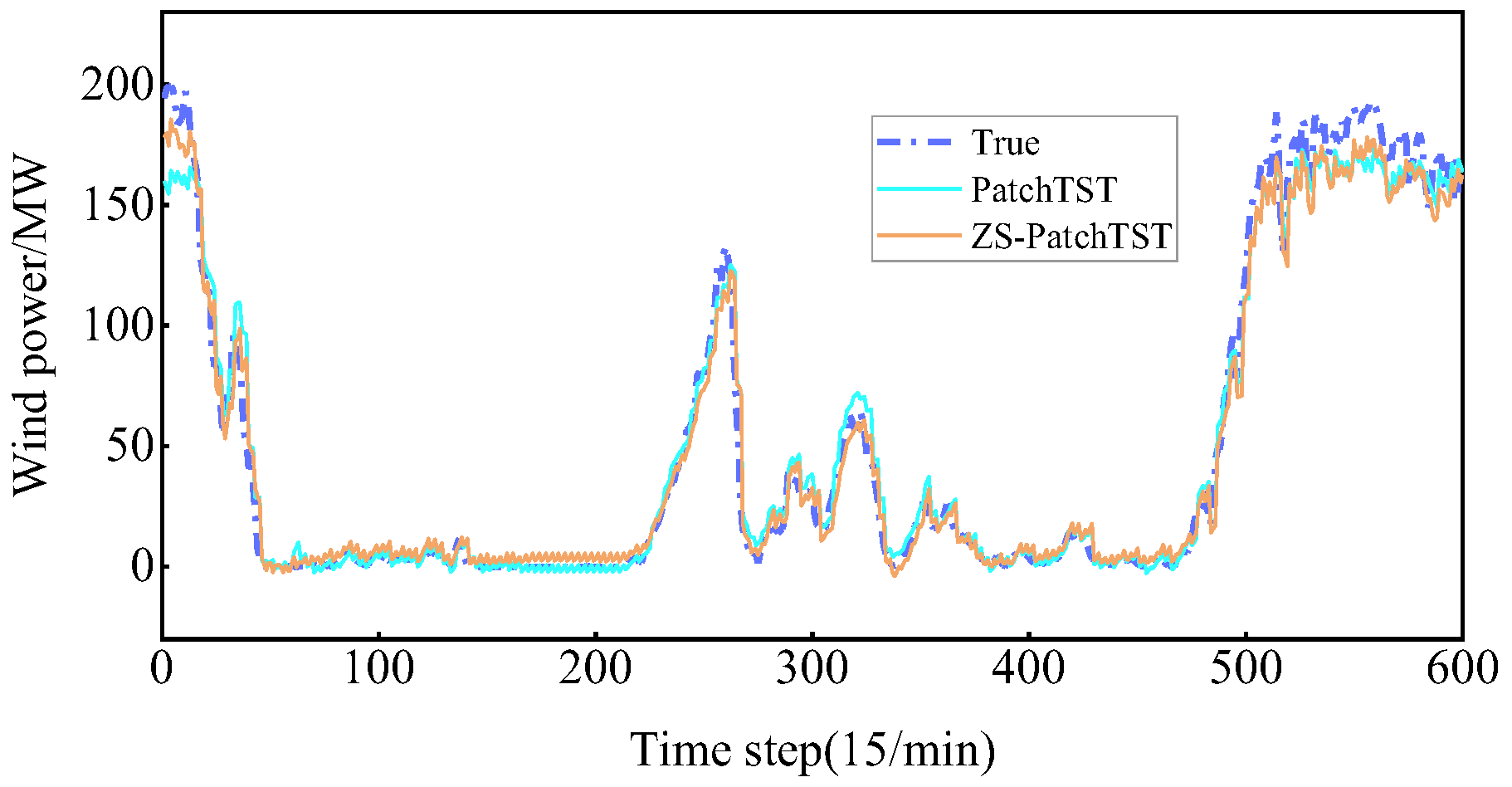
4.3.1. Impact of ZS Standardization on Prediction Results

To reduce the impact of wind power data distribution shift on model prediction accuracy, ZS standardization is introduced based on the PatchTST model. The comparison of the prediction curves (600 data points) between the ZS-PatchTST and PatchTST models is shown in Figure 8. The prediction accuracy of the ZS-PatchTST and PatchTST models for the entire test set is shown in

Table 6. Comparison of prediction accuracy between ZS-PatchTST and PatchTST models test set.

Model	MAE/MW	RMSE/MW	R2/%
PatchTST	9.26	15.12	94.97
ZS-PatchTST	8.23	13.00	96.28

.

In Figure 8, the orange solid line represents the prediction results of the ZS-PatchTST model, while the blue solid line represents the prediction results of the PatchTST model. The ZS-PatchTST model’s prediction curve fits the actual value curve more closely. From Table 6, it can be seen that the MAE and RMSE of the ZS-PatchTST model decreased by 1.03 MW and 2.12 MW, respectively, compared to the PatchTST model, and the R² increased by 1.31%. This demonstrates that Z-score standardization can reduce the adverse effects of wind power data distribution shift on model prediction accuracy.

4.3.2. Impact of DT Standardization on Prediction Results

Based on the ZS module, the DT algorithm is introduced to address the window data distribution shift issue. A simulation comparison analysis was conducted with several similar algorithms. The prediction results (600 data points) are shown in Figure 9, and the prediction accuracy for the test set is shown in

Table 7. Prediction accuracy comparison of various models.

Model	MAE/MW	RMSE/MW	R2/%
ZS-PatchTST	8.23	13.00	96.28
ZS-RV-PatchTST	6.30	11.99	96.84
ZS-ZS-PatchTST	6.26	11.98	96.84
ZS-DT-PatchTST	5.95	10.89	97.38

.

In the zoomed-in area of Figure 9, the fit of the curves improved after addressing the wind power data window distribution shift problem using ZS, RV, and DT compared to the ZS-PatchTST model, which did not address the window problem. From Table 7, it can be seen that the MAE and RMSE of the ZS-DT-PatchTST model decreased by 2.28 MW and 2.11 MW, respectively, compared to the ZS-PatchTST model, and R² increased by 1.10%. The MAE and RMSE of the ZS-DT-PatchTST model decreased by 0.35 MW and 1.10 MW, respectively, compared to the ZS-RV-PatchTST model, and R² increased by 0.54%. Similarly, the MAE and RMSE of the ZS-DT-PatchTST model decreased by 0.31 MW and 1.09 MW, respectively, compared to the ZS-ZS-PatchTST model, and R² increased by 0.54%. Thus, it is verified that the deviation of wind power data window distribution leads to a decrease in model prediction accuracy, and the DT algorithm is superior to ZS and RV in solving the problem of wind power data window distribution deviation.

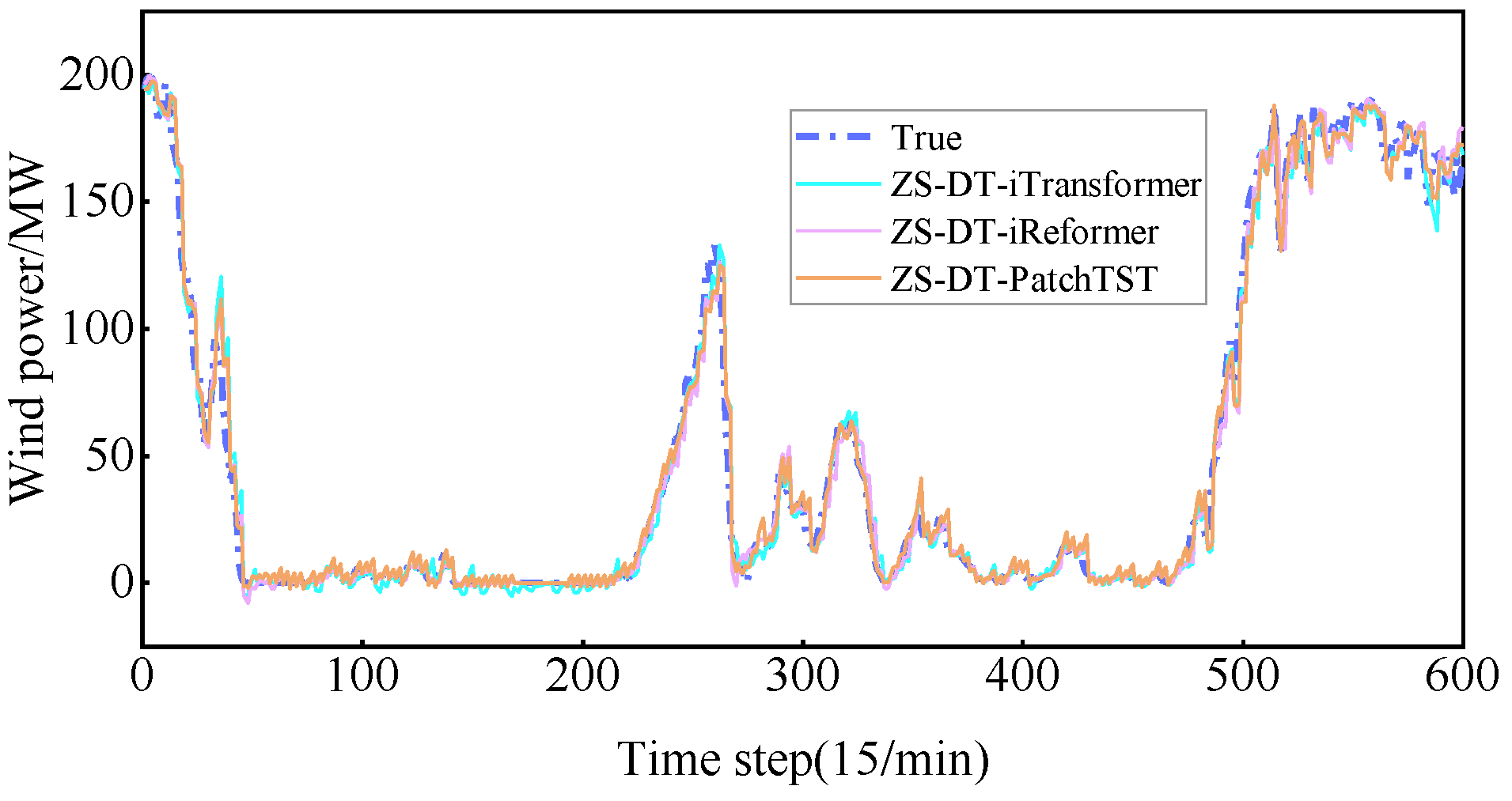
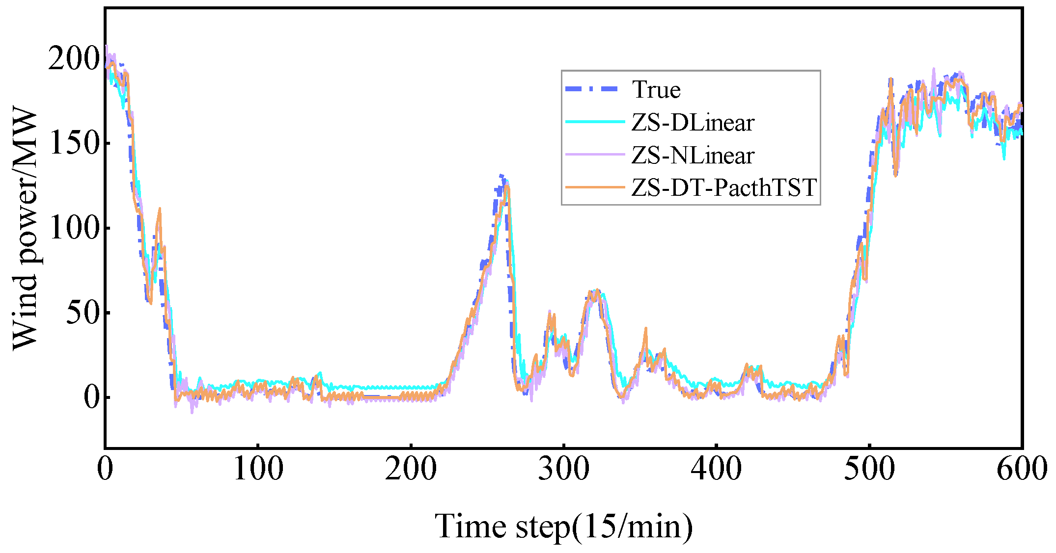
4.3.3. Comparative Analysis of ZS-DT-PatchTST and Common Time Series Prediction Models

(1)

Comparative analysis of ZS-DT-PatchTST model and former series models.

The proposed ZS-DT method can be integrated with common former series models. ZS-DT is introduced into point–input models such as Transformer, Informer, Reformer, and NsTransformer, as well as channel-level input models such as iTransformer and iReformer. The prediction curves of these models compared to the ZS-DT-PatchTST model are shown in Figure 10 and Figure 11, and the prediction accuracy for the test set is shown in

Table 8. Prediction accuracy on test set for various models.

Model	MAE/MW	RMSE/MW	R2/%
ZS-DT-Transformer	8.27	12.95	96.33
ZS-DT-Informer	7.98	12.45	96.61
ZS-DT-Reformer	7.11	12.18	96.74
ZS-DT-NsTransformer	6.60	11.64	97.02
ZS-DT-iTransformer	6.20	11.61	97.07
ZS-DT-iReformer	6.25	11.81	96.93
ZS-DT-PatchTST	5.95	10.89	97.38

.

In Table 8, the MAE and RMSE of the ZS-DT-PatchTST model are compared with those of various former series models, showing significant improvements. Compared to the ZS-DT-Transformer model, the MAE and RMSE of the ZS-DT-PatchTST model are reduced by 2.32 MW and 2.06 MW, respectively, with an R² increase of 1.05%. Compared to the ZS-DT-Informer model, the MAE and RMSE are reduced by 2.03 MW and 1.56 MW, respectively, with an R² increase of 0.77%. Compared to the ZS-DT-Reformer model, the MAE and RMSE are reduced by 1.16 MW and 1.29 MW, respectively, with an R² increase of 0.64%. Compared to the ZS-DT-NsTransformer model, the MAE and RMSE are reduced by 0.65 MW and 0.75 MW, respectively, with an R² increase of 0.36%. Compared to the ZS-DT-iTransformer model, the MAE and RMSE are reduced by 0.25 MW and 0.72 MW, respectively, with an R² increase of 0.31%. Compared to the ZS-DT-iReformer model, the MAE and RMSE are reduced by 0.30 MW and 0.92 MW, respectively, with an R² increase of 0.45%. From this analysis, it can be concluded that the former models using Patch for local input achieve higher prediction accuracy than those using point input or channel input.

(2)

Comparison between ZS-DT-PatchTST model and linear models.

In recent years, DLinear and NLinear linear layer models have been widely used in the field of time series forecasting, achieving high prediction accuracy with simple linear layers. The comparison between the ZS-DT-PatchTST model and the ZS-NLinear and ZS-DLinear models is shown in Figure 12, and the test set prediction accuracy is shown in

Table 9. Prediction accuracy on the test set for ZS-DT-PT vs. ZS-DLinear and ZS-NLinear models.

Model	MAE/MW	RMSE/MW	R2/%
ZS-DLinear	10.66	15.75	94.55
ZS-NLinear	7.19	12.92	96.33
ZS-DT-PatchTST	5.95	10.89	97.38

.

In Table 9, the ZS-DT-PatchTST model’s MAE and RMSE are reduced by 4.71 MW and 4.86 MW, respectively, compared to the ZS-DLinear model, with an average increase in R² of 2.83%. When compared to the ZS-NLinear model, the ZS-DT-PatchTST model’s MAE and RMSE are reduced by 1.24 MW and 2.03 MW, respectively, with an average increase in R² of 1.05%. This demonstrates that the proposed model has higher prediction accuracy.

(3)

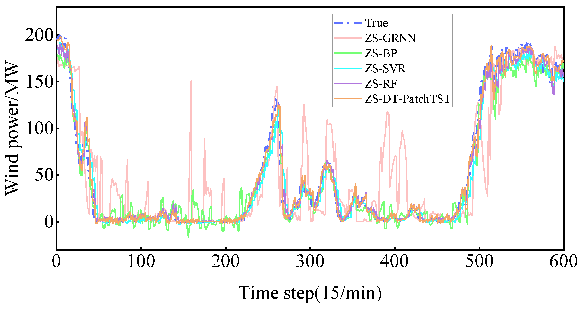
Comparison between the ZS-DT-PatchTST model and traditional machine learning models.

The proposed model in this paper is compared with the traditional network general regression neural network (GRNN) model, backpropagation (BP) model, support vector regression (SVR) model, and random forest (RF) model, and the comparison of the model prediction curves (600 data points) is shown in Figure 13. The test set prediction accuracy comparison is shown in

Table 10. Comparison of prediction accuracy between ZS-DT-PatchTST and traditional machine learning model test set.

Model	MAE/MW	RMSE/MW	R2/%
ZS-GRNN	25.51	38.73	70.10
ZS-BP	11.12	18.08	92.82
ZS-SVR	9.56	16.13	94.29
ZS-RF	7.42	12.72	96.45
ZS-DT-PatchTST	5.95	10.89	97.38

.

In Table 10, the ZS-DT-PatchTST model reduces the MAE and RMSE by 19.56 MW and 27.84 MW, respectively, and improves the R² by 27.28% compared to the ZS-GRNN model. The MAE and RMSE reduce the MAE and RMSE by 5.17 MW and 7.19 MW, respectively, and improve the R² by 4.56% compared to the ZS-BP model. The MAE and RMSE reduce the MAE and RMSE by 3.61 MW and 5.24 MW, respectively, and improve the R² by 3.09% compared to the ZS-SVR model. Compared with the ZS-RF model, the MAE and RMSE are reduced by 1.47 MW and 1.83 MW, respectively, and the R² is improved by 0.93%, thus verifying that the proposed model in this paper still has an advantage over the traditional machine learning algorithm.

(4)

Comparison of ZS-DT-PatchTST with LSTM and GRU models.

LSTM and GRU models are variants of recurrent neural networks (RNN). The ZS-DT-PatchTST model proposed in this paper is a variant of the Transformer model. Unlike the LSTM and GRU models, it adopts the PatchTST model on the basis of the ZS-DT to solve the problem of offsetting the distribution of the wind power data; it establishes local correlation and extracts the local information through the mechanism of multi-attention, enabling parallel processing without the need to transfer the information step-by-step through the time steps. It is of some significance to compare with LSTM and GRU series models in the field of ultra-short-term time series prediction. Therefore, a comparison analysis between the proposed ZS-DT-PatchTST model and LSTM and GRU models was conducted. The prediction curves (600 data points) are shown in Figure 14, and the comparison of prediction accuracy on the test set is presented in

Table 11. Comparison of test set prediction accuracy between ZS-DT-PT and LSTM, GRU series models.

Model	MAE/MW	RMSE/MW	R2/%
ZS-TCN-BiGRU	10.00	15.09	94.99
ZS-LSTM	9.21	13.10	96.22
ZS-GRU	8.86	12.76	96.41
ZS-BiLSTM	6.99	11.94	96.86
ZS-DT-PatchTST	5.95	10.89	97.38

.

In Table 11, the MAE and RMSE of the ZS-DT-PatchTST model compared to the ZS-TCN-BiGRU model decreased by 4.05 MW and 4.20 MW, respectively, and the R² increased by 2.39%. The MAE and RMSE of the ZS-DT-PatchTST model compared to the ZS-LSTM model decreased by 3.26 MW and 2.21 MW, respectively, and the R² increased by 1.16%. The MAE and RMSE of the ZS-DT-PatchTST model compared to the ZS-GRU model decreased by 2.91 MW and 1.87 MW, respectively, and the R² increased by 0.97%. The MAE and RMSE of the ZS-DT-PatchTST model compared to the ZS-BiLSTM model decreased by 1.04 MW and 1.05 MW, respectively, and the R² increased by 0.52%. This verifies that the ZS-DT-PatchTST model proposed in this paper has higher prediction accuracy compared to the LSTM and GRU series models.

4.3.4. Prediction Accuracy Analysis of Different Datasets

The error analysis of the test set prediction results of wind power dataset 2 with an acquisition frequency of 5 min was performed, and the ZS-DT-PatchTST model proposed in this paper was compared with the former family of models (Autoformer, Informer). The LSTM and GRU family of models (TCN-BiGRU, LSTM), the linear model (DLnear, NLinear), and traditional machine learning models (GRNN, SVR) were compared, and the comparison of prediction accuracy of different model test sets for wind power dataset 2 is shown in

Table 12. Comparison of prediction accuracies of different model test sets for wind power dataset 2.

Model	MAE/MW	RMSE/MW	R2/%
ZS–Autoformer	3.11	4.82	95.33
ZS–Informer	2.99	4.50	95.99
ZS-TCN-BiGRU	3.31	4.57	95.79
ZS-LSTM	2.74	4.33	96.22
ZS-DLinear	5.13	7.28	90.10
ZS-NLinear	2.76	4.29	96.31
ZS-GRNN	3.83	5.87	93.17
ZS-SVR	3.36	5.29	94.44
ZS-DT-PatchTST	2.27	3.84	97.03

.

In Table 12, the MAE and RMSE of the ZS-DT-PatchTST model compared with the ZS–Autoformer and ZS–Informer models decreased by 0.78 MW and 0.82 MW on average, and the R² increased by 1.37% on average. Compared with ZS-LSTM and ZS-TCN-BiGRU models, MAE and RMSE decreased by 0.755 MW and 0.61 MW on average, and the R² increased by 1.025% on average. Compared with ZS-DLinear and ZS-NLinear models, MAE and RMSE decreased by 1.675 MW and 1.945 MW, respectively, and R² increased by 3.825% on average. Compared with ZS-GRNN and ZS-SVR models, MAE and RMSE decreased by 1.325 MW and 1.74 MW, and R² increased by 3.225% on average. Thus, it is verified that the model proposed in this paper can still achieve a high prediction accuracy on a smaller wind power dataset 2 with a collection frequency of 5 min.

5. Conclusions

When using point-by-point data input in former series models for wind power prediction, the prediction accuracy decreases due to the distribution shift in wind power data and the inability to extract wind power data point local information. To address these issues, this paper proposes combining ZS and DT to mitigate the distribution shift in wind power data and using Patch to integrate correlated data points into multiple Patches. The multi-head attention mechanism is then utilized to explore the correlation between Patches for feature extraction, thus improving the model’s prediction accuracy. The experimental analysis leads to the following conclusions:

• By incorporating ZS normalization into the PatchTST model to address the distribution shift between training and testing datasets, the MAE and RMSE of the ZS-PatchTST model decreased by 1.03 MW and 2.12 MW, respectively, while the R² increased by 1.31%. This validates that Z-score normalization can effectively mitigate the impact of distribution shift on model prediction accuracy.
• Building on the solution to the training and testing dataset distribution shift, ZS, RV, and DT were introduced to handle the distribution shift between data windows. The MAE and RMSE of the ZS-DT-PatchTST model decreased by 2.28 MW and 2.11 MW, respectively, compared to the ZS-PatchTST model, and R² increased by 1.10%. The MAE and RMSE of the ZS-DT-PatchTST model compared to the ZS-RV-PatchTST model decreased by 0.35 MW and 1.10 MW, respectively, with an R² increase of 0.54%. Similarly, compared to the ZS-ZS-PatchTST model, the MAE and RMSE decreased by 0.31 MW and 1.09 MW, with an R² increase of 0.54%. This indicates that the problem of window distribution offset in wind power data can lead to a decrease in model prediction accuracy, and the DT model is more effective than ZS and RV in solving the problem of window distribution offset.
• Taking two wind power dataset 1 and wind power dataset 2 with different collection frequencies as benchmarks, the prediction error analysis of this paper’s model and the common time-series prediction model show that the prediction accuracy of this paper’s model is at the highest level in the test set. The MAE and RMSE of the proposed model in wind power dataset 1 are 5.95 MW and 10.89 MW, respectively, with an R² of 97.38%, and the MAE and RMSE of the proposed model in wind power dataset 2 are 2.27 MW and 3.84 MW, respectively, with an R² of 97.03%. Thus, using ZS-DT to deal with the problem of wind power data distribution bias and then combined with the PatchTST model to extract local features of wind power data for wind power prediction has certain advantages.
• Although the Z-score algorithm can be standardized by obtaining the mean and variance, thus reducing the impact of the distributional bias between the training set and the test set on the accuracy of model prediction, when the wind power data with a large proportion of anomalies are used, it will obviously affect the value of the mean and variance, which will, to a certain extent, affect the standardization of the dataset and the prediction of the model. Therefore, the selection of different standardization methods for different datasets needs to be followed up with more in-depth research.

References

- Chang, Y.; Yang, H.; Chen, Y.X.; Zhou, M.R.; Yang, H.B.; Wang, Y.; Zhang, Y.R. A Hybrid Model for Long-Term Wind Power Forecasting Utilizing NWP Subsequence Correction and Multi-Scale Deep Learning Regression Methods. IEEE Trans. Sustain. Energy 2024, 15, 263–275. [Google Scholar] [CrossRef]
- Ahmadi, A.; Nabipour, M.; Mohammadi-Ivatloo, B.; Amani, A.M.; Rho, S.; Piran, M.J. Long-Term Wind Power Forecasting Using Tree-Based Learning Algorithms. IEEE Access 2020, 8, 151511–151522. [Google Scholar] [CrossRef]
- Papadopoulos, P.; Fallahi, F.; Yildirim, M.; Ezzat, A.A. Joint Optimization of Production and Maintenance in Offshore Wind Farms: Balancing the Short- and Long-Term Needs of Wind Energy Operation. IEEE Trans. Sustain. Energy 2024, 15, 835–846. [Google Scholar] [CrossRef]
- Xu, H.S.; Fan, G.L.; Kuang, G.F.; Song, Y.P. Construction and Application of Short-Term and Mid-Term Power System Load Forecasting Model Based on Hybrid Deep Learning. IEEE Access 2023, 11, 37494–37507. [Google Scholar] [CrossRef]
- Sharma, A.; Jain, S.K. A Novel Two-Stage Framework for Mid-Term Electric Load Forecasting. IEEE Trans. Ind. Inform. 2024, 20, 247–255. [Google Scholar] [CrossRef]
- Sun, Z.X.; Zhao, S.S.; Zhang, J.X. Short-Term Wind Power Forecasting on Multiple Scales Using VMD Decomposition, K-Means Clustering and LSTM Principal Computing. IEEE Access 2019, 7, 166917–166929. [Google Scholar] [CrossRef]
- Zhao, M.L.; Zhou, X. Multi-Step Short-Term Wind Power Prediction Model Based on CEEMD and Improved Snake Optimization Algorithm. IEEE Access 2024, 12, 50755–50778. [Google Scholar] [CrossRef]
- Sun, Y.; Yang, J.J.; Zhang, X.T.; Hou, K.Y.; Hu, J.Y.; Yao, G.Z. An Ultra-Short-Term Wind Power Forecasting Model Based on EMD-EncoderForest-TCN. IEEE Access 2024, 12, 60058–60069. [Google Scholar] [CrossRef]
- Xu, H.L.; Zhang, Y.R.; Zhen, Z.; Xu, F.; Wang, F. Adaptive Feature Selection and GCN With Optimal Graph Structure-Based Ultra-Short-Term Wind Farm Cluster Power Forecasting Method. IEEE Trans. Ind. Appl. 2024, 60, 1804–1813. [Google Scholar] [CrossRef]
- Li, Z.; Ye, L.; Zhao, Y.N.; Pei, M.; Lu, P.; Li, Y.L.; Dai, B.H. A Spatiotemporal Directed Graph Convolution Network for Ultra-Short-Term Wind Power Prediction. IEEE Trans. Sustain. Energy 2023, 14, 39–54. [Google Scholar] [CrossRef]
- An, G.Q.; Jiang, Z.Y.; Cao, X.; Liang, Y.F.; Zhao, Y.Y.; Li, Z.; Dong, W.C.; Sun, H.X. Short-Term Wind Power Prediction Based on Particle Swarm Optimization-Extreme Learning Machine Model Combined With Adaboost Algorithm. IEEE Access 2021, 9, 94040–94052. [Google Scholar] [CrossRef]
- Zhou, W.B.; Xin, M.; Wang, Y.L.; Yang, C.; Liu, S.S.; Zhang, R.Z.; Liu, X.D.; Zhou, L.N. An Ultra-Short-Term Wind Power Prediction Method Based On CNN-LSTM. In Proceedings of the 2024 IEEE 7th Advanced Information Technology, Electronic and Automation Control Conference (IAEAC), Chongqing, China, 15–17 March 2024; pp. 1007–1011. [Google Scholar]
- Pan, C.Y.; Wen, S.L.; Zhu, M.; Ye, H.L.; Ma, J.J.; Jiang, S. Hedge Backpropagation Based Online LSTM Architecture for Ultra-Short-Term Wind Power Forecasting. IEEE Trans. Power Syst. 2024, 39, 4179–4192. [Google Scholar] [CrossRef]
- Abedinia, O.; Ghasemi-Marzbali, A.; Shafiei, M.; Sobhani, B.; Gharehpetian, G.B.; Bagheri, M. Wind Power Forecasting Enhancement Utilizing Adaptive Quantile Function and CNN-LSTM: A Probabilistic Approach. IEEE Trans. Ind. Appl. 2024, 60, 4446–4457. [Google Scholar] [CrossRef]
- Saeed, A.; Li, C.S.; Danish, M.; Rubaiee, S.; Tang, G.; Gan, Z.H.; Ahmed, A. Hybrid Bidirectional LSTM Model for Short-Term Wind Speed Interval Prediction. IEEE Access 2020, 8, 182283–182294. [Google Scholar] [CrossRef]
- Sheng, A.D.; Xie, L.W.; Zhou, Y.X.; Wang, Z.; Liu, Y.C. A Hybrid Model Based on Complete Ensemble Empirical Mode Decomposition with Adaptive Noise, GRU Network and Whale Optimization Algorithm for Wind Power Prediction. IEEE Access 2023, 11, 62840–62854. [Google Scholar] [CrossRef]
- Yin, K.; Yang, Y.; Yao, C.P.; Yang, J.W. Long-Term Prediction of Network Security Situation Through the Use of the Transformer-Based Model. IEEE Access 2022, 10, 56145–56157. [Google Scholar] [CrossRef]
- Han, C.J.; Ma, T.; Gu, L.H.; Cao, J.D.; Shi, X.L.; Huang, W.; Tong, Z. Asphalt Pavement Health Prediction Based on Improved Transformer Network. IEEE Trans. Int. Transp. Syst. 2023, 24, 4482–4493. [Google Scholar] [CrossRef]
- Fauzi, N.A.; Ali, N.H.N.; Ker, P.J.; Thiviyanathan, V.A.; Leong, Y.S.; Sabry, A.H.; Jamaludin, M.Z.B.; Lo, C.K.; Mun, L.H. Fault Prediction for Power Transformer Using Optical Spectrum of Transformer Oil and Data Mining Analysis. IEEE Access 2020, 8, 136374–136381. [Google Scholar] [CrossRef]
- Wang, X.H.; Xia, M.C.; Deng, W.W. MSRN-Informer: Time Series Prediction Model Based on Multi-Scale Residual Network. IEEE Access 2023, 11, 65059–65065. [Google Scholar] [CrossRef]
- Bi, C.; Ren, P.; Yin, T.; Zhang, Y.; Li, B.; Xiang, Z. An Informer Architecture-Based Ionospheric foF2 Model in the Middle Latitude Region. IEEE Geosci. Remote Sens. Lett. 2022, 19, 1005305. [Google Scholar] [CrossRef]
- Pan, G.L.; Wu, Q.H.; Ding, G.R.; Wang, W.; Li, J.; Zhou, B. An Autoformer-CSA Approach for Long-Term Spectrum Prediction. IEEE Wireless Commun. Lett. 2023, 12, 1647–1651. [Google Scholar] [CrossRef]
- Yang, C.; Yang, C.J.; Zhang, X.M.; Zhang, J.F. Multisource Information Fusion for Autoformer: Soft Sensor Modeling of FeO Content in Iron Ore Sintering Process. IEEE Trans. Ind. Inform. 2023, 19, 11584–11595. [Google Scholar] [CrossRef]
- Nie, Y.Q.; Nguyen, N.H.; Sinthong, P.; Kalagnanam, J. A Time Series is Worth 64 Words: Long-Term Forecasting with TransformErs. arXiv 2022, arXiv:2211.14730. [Google Scholar]
- Liu, Y.; Wang, W.; Chang, L.Q.; Tang, J. MSWI Multi-Temperature Prediction Based on Patch Time Series Transformer. In Proceedings of the 2024 36th Chinese Control and Decision Conference (CCDC), Xi’an, China, 25–27 May 2024; pp. 2369–2373. [Google Scholar]
- Zhang, L.L.; Shi, Y.; Jin, X.; Xu, S.J.; Wang, C.Y.; Liu, F.X. Water Quality Index Forecasting via Transformers: A Comparative Experimental Study. In Proceedings of the 2023 China Automation Congress (CAC), Chongqing, China, 17–19 November 2023; pp. 8114–8119. [Google Scholar]
- Yaro, A.S.; Maly, F.; Prazak, P.; Malý, K. Outlier Detection Performance of a Modified Z-Score Method in Time-Series RSS Observation with Hybrid Scale Estimators. IEEE Access 2024, 12, 12785–12796. [Google Scholar] [CrossRef]
- Liu, L.; Li, C.X.; Li, X.; Ge, Q.B. State of Energy Estimation of Electric Vehicle Based on GRU-RNN. In Proceedings of the 2022 37th Youth Academic Annual Conference of Chinese Association of Automation (YAC), Beijing, China, 19–20 November 2022; pp. 115–120. [Google Scholar]
- Kim, T.; Kim, J.; Tae, Y.; Park, C.; Choi, J.; Choo, J. Reversible Instance Normalization for Accurate Time-Series Forecasting Against Distribution Shift. In Proceedings of the International Conference on Learning Representations (ICLR), Virtual Event, 25–29 April 2022; pp. 1–25. [Google Scholar]
- Liu, Y.; Wu, H.X.; Wang, J.M.; Long, M.S. Non-stationary Transformers: Exploring the Stationarity in Time Series Forecasting. Adv. Neural Inf. Process. Syst. 2022, 35, 9881–9893. [Google Scholar]
- Jha, A.; Dorkar, O.; Biswas, A.; Emadi, A. iTransformer Network Based Approach for Accurate Remaining Useful Life Prediction in Lithium-Ion Batteries. In Proceedings of the 2024 IEEE Transportation Electrification Conference and Expo (ITEC), Chicago, IL, USA, 19–21 June 2024; pp. 1–8. [Google Scholar]
- Fan, W.; Wang, P.Y.; Wang, D.K.; Wang, D.J.; Zhou, Y.C.; Fu, Y.J. Dish-Ts: A General Paradigm for Alleviating Distribution Shift in Time Series Forecasting. In Proceedings of the 2023 37th AAAI Conference on Artificial Intelligence, Washington DC, USA, 7–14 February 2023; pp. 7522–7529. [Google Scholar]
- Wu, J.J.; Guo, Y. Degradation Prediction of Proton Exchange Membrane Fuel Cell Considering Distribution Shift. In Proceedings of the 2023 7th International Conference on Electrical, Mechanical and Computer Engineering (ICEMCE), Xian, China, 20–22 October 2023; pp. 443–447. [Google Scholar]
- Kwok, W.M.; Streftaris, G.; Dass, S.C. A Novel Target Value Standardization Method Based on Cumulative Distribution Functions for Training Artificial Neural Networks. In Proceedings of the 2023 IEEE 13th Symposium on Computer Applications & Industrial Electronics (ISCAIE), Penang, Malaysia, 20–21 May 2023; pp. 250–255. [Google Scholar]
- LI, G.; Ning, X.; Gong, W.L.; Zhou, L.H.; Guo, W.W. Evaluation Method of Distribution Network State Based on IT-II-Fuzzy K-means Clustering Algorithm for Imbalanced Data under PIOT. In Proceedings of the 2022 Asian Conference on Frontiers of Power and Energy (ACFPE), Chengdu, China, 21–23 October 2022; pp. 211–215. [Google Scholar]
- Shi, Z.H.; Xiao, J.; Jiang, J.H.; Zhang, Y.; Zhou, Y.H. Identifying Reliability High-Correlated Gates of Logic Circuits with Pearson Correlation Coefficient. IEEE Trans. Circuits Syst. 2024, 71, 2319–2323. [Google Scholar] [CrossRef]
- Zhao, Q.C.; Zhang, Y.Y.; Zhao, Z.Q.; Nie, Z.P. A Joint Inversion Approach of Electromagnetic and Acoustic Data Based on Pearson Correlation Coefficient. IEEE Trans. Geosci. Remote Sens. 2024, 62, 4704911. [Google Scholar] [CrossRef]
- Calik, N.; Güneş, F.; Koziel, S.; Pietrenko-Dabrowska, A.; Belen, M.A.; Mahouti, P. Deep-Learning-Based Precise Characterization of Microwave Transistors Using Fully-Automated Regression Surrogates. Sci. Rep. 2023, 13, 1445. [Google Scholar] [CrossRef]
- Hanifi, S.; Cammarono, A.; Zare-Behtash, H. Advanced Hyperparameter Optimization of Deep Learning Models for Wind Power Prediction. Renew. Energy 2024, 221, 119700. [Google Scholar] [CrossRef]