Considerations Regarding the Middle Power Asynchronous Motors for Railway Electrical Traction

Abstract

In modern electric traction, direct current traction motors have been replaced with asynchronous motors with a short-circuited rotor. The justification is that asynchronous motors are more reliable, cheaper, and have smaller weights and dimensions, so they are more sustainable. In order to start and adjust the speed required in traction, these motors are powered from the contact line using a transformer and a static voltage and frequency converter. As a result, you can use green electricity produced with wind power plants or solar energy converted with photovoltaic panels, increasing sustainability because the consumption of traditional fuels is reduced. This paper presents various simulations emphasizing the negative effects of the distorting regime, with concrete results. The quality of the simulations carried out is increased by using a mathematical model, which uses the variable parameters of the motor dependent on the modulation of the current and the magnetic saturation. In modern 1500 kW electric locomotives, the traction motors are powered by static converters, which means an increase in losses when operating at nominal load on the motors by 38.7 kW and 217.8 kVAR compared to the sinusoidal three-phase power supply. Thus, the research carried out provides qualitatively and quantitatively correct simulations of the non-sinusoidal regime related to the asynchronous traction motor in order to increase the sustainability of this traction system.

1. Introduction

This study presents the results of research on the middle power asynchronous motor used in electric traction in the case of feeding from a static voltage and frequency converter [1,2,3,4].

In the specialized literature [5,6,7], one can find papers that describe the operation of asynchronous motors fed from static converters, but this paper presents concrete results regarding the sustainability of the analyzed traction motor.

An in-depth study of the operation of the asynchronous motor–static converter assembly can establish a constructive version of a sustainable motor, realized through advantageous manufacturing costs and minimal operating expenses.

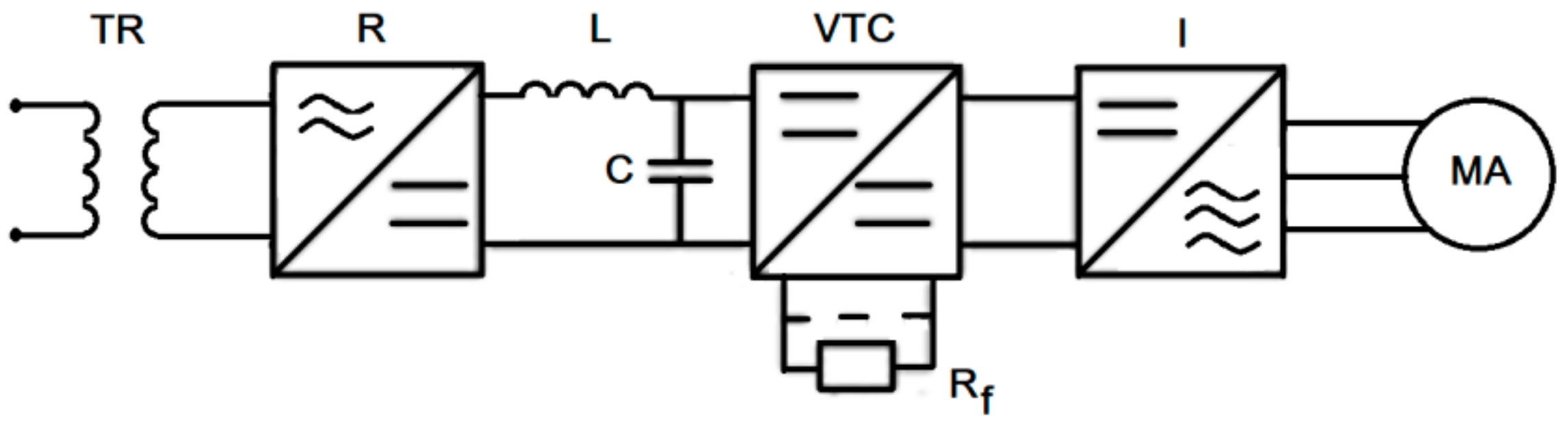
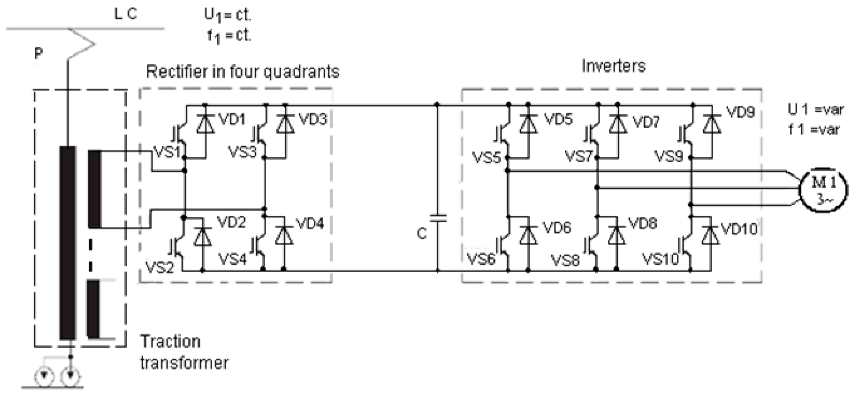
The power circuit of the electric locomotive, shown in Figure 1, consists of the following: TR—the main transformer, R—rectifier, L+C filter, VTC—direct voltage variator, I—inverter, and MA—asynchronous traction motor.

Starting with this observation, it follows that there is a need for the design and construction of the asynchronous traction motor to be performed while considering the consequences of the deforming regime caused by the supply from the static converter. Increasing the sustainability of the static converter–asynchronous traction motor assembly requires us to establish the optimal motor option [5,6,7,8,9,10,11], so that for the selected static converter, the operating characteristics of the asynchronous motor meet the operating requirements and result in a judicious use of existing energy resources.

When establishing the effects of the deforming regime, an important problem is the analysis of the current and power voltage waves, associated with the static converter–asynchronous motor assembly, as well as the establishment of the important harmonics to obtain a small distortion factor.

By carrying out some simulations on the basis of a mathematical model from the literature, the operation characteristics can be established very exactly, qualitatively and quantitatively.

2. Mathematical Model of the Traction Asynchronous Motor

The quality of the simulations carried out emphasizes the behavior of the traction asynchronous motor, supplied by a static converter, both in a steady regime and in a dynamic one [12,13,14,15,16].

The operation characteristics obtained in the case of supplying from a static voltage and frequency converter are compared to the classical ones, where the same motor is supplied from a three-phase network, with symmetrical and sinusoidal voltages. Thus, we can anticipate the behavior of the motor and the differences occurring in the two situations.

The simulations have been carried out by using a mathematical model, with two axes equations, rotor quantities related to the stator [17,18,19,20], written in a reference frame, which is fixed against the stator (ω_B = 0),

$${\underset{¯}{u}}_s={\displaystyle \frac{2}{3}}\left(u_A+a{u}_B+a^2{u}_C\right)$$

(1)

$${\underset{¯}{u}}_s=u_{ds}+j{u}_{qs}$$

(2)

$$\begin{array}{c}{u}_{ds}=R_s{i}_{ds}+{\displaystyle \frac{d}{dt}}\left(L_{ds}{i}_{ds}+L_{dsr}{i^{\prime }}_{dr}\right)-\mathsf{\omega }(L_{qs}{i}_{qs}+L_{qsr}{i^{\prime }}_{qr})\\ u_{qs}=R_s{i}_{qs}+{\displaystyle \frac{d}{dt}}\left(L_{qs}{i}_{qs}+L_{qsr}{i^{\prime }}_{qr}\right)-\mathsf{\omega }(L_{ds}{i}_{ds}+L_{dsr}{i^{\prime }}_{dr})\\ {u^{\prime }}_{dr}=R_r{i^{\prime }}_{dr}+{\displaystyle \frac{d}{dt}}\left(L_{drs}{i}_{ds}+L_{dr}{i^{\prime }}_{dr}\right)\\ {u\prime }_{qr}=R_r{i\prime }_{qr}+{\displaystyle \frac{d}{dt}}\left(L_{qrs}{i}_{qs}+L_{qr}{i^{\prime }}_{qr}\right)\end{array}$$

(3)

This mathematical model can also be re-written as state equations as follows:

$$\begin{array}{c}{\displaystyle \frac{d}{dt}}\left[\begin{array}{c}{i}_{ds}\\ i_{qs}\\ i_{dr}^{\prime }\\ i_{qr}^{\prime }\end{array}\right]={\displaystyle \frac{1}{L_s{L}_r^{\prime }-L_{sh}^2}}\left[\begin{array}{cccc}-R_s{L}_r^{\prime }& \mathsf{\omega }{L}_{sh}^2& R_r^{\prime }{L}_{sh}& \mathsf{\omega }{L}_r^{\prime }{L}_{sh}\\ -\mathsf{\omega }{L}_{sh}^2& -R_s{L}_r^{\prime }& -\mathsf{\omega }{L}_r^{\prime }{L}_{sh}& R_r^{\prime }{L}_{sh}\\ R_s{L}_{sh}& -\mathsf{\omega }{L}_s{L}_{sh}& -R_r^{\prime }{L}_s& -\mathsf{\omega }{L}_s{L}_r^{\prime }\\ \mathsf{\omega }{L}_s{L}_{sh}& R_s{L}_{sh}& \mathsf{\omega }{L}_s{L}_r^{\prime }& -R_r^{\prime }{L}_s\end{array}\right]·\left[\begin{array}{c}{i}_{ds}\\ i_{qs}\\ i_{dr}^{\prime }\\ i_{qr}^{\prime }\end{array}\right]+\\ +{\displaystyle \frac{1}{L_s{L}_r^{\prime }-L_{sh}^2}}\left[\begin{array}{cc}{L}_r^{\prime }& 0\\ 0& L_r^{\prime }\\ -L_{sh}& 0\\ 0& -L_{sh}\end{array}\right]·\left[\begin{array}{c}{u}_{ds}\\ u_{qs}\end{array}\right]\end{array}$$

(4)

The motion equation is added to them:

$${\displaystyle \frac{d\mathsf{\omega }}{dt}}={\displaystyle \frac{p}{J}}\left({\displaystyle \frac{3}{2}}p{L}_{sh}(i_{qs}{i}_{dr}^{\prime }-i_{ds}{i}_{qr}^{\prime })-m_r\right)$$

(5)

where the first term inside the bracket is the electromagnetic torque:

$$m={\displaystyle \frac{3}{2}}p{L}_{sh}(i_{qs}{i}_{dr}^{\prime }-i_{ds}{i}_{qr}^{\prime })$$

(6)

–

$R_s, L_s$—the total resistance and inductance on one phase in the stator;

–

$R_r^{\prime }, L_r^{\prime }$—the resistance and total inductance on one phase in the rotor in reported sizes;

–

ω—the electric angular speed of the rotor;

–

$L_{sh}$—the main cyclic inductance;

–

$u_A, u_B, u_C$—the voltages on the three phases of the motor;

–

$a=e^{j·2\mathsf{\pi }\prime 3}$—the operator (rotating the phasor by 2π/3 in the trigonometric sense), used in the simplified complex calculation method operator;

–

$u_{ds}, u_{qs}$—the components along the two axes d, q of the complex phasor ${\underset{¯}{u}}_s$ of the stator voltage;

–

$i_{ds}, i_{qs}$—the components along the d, q axes of the stator current phasor $i_s$;

–

$i_{dr}^{\prime }, i_{qr}^{\prime }$—the components along the d, q axes of the reported rotor current phasor $i_r^{\prime }$.

Knowing the machine parameters, its rated data, and the resistant shaft torque by integrating one of the systems presented above the following dependences during the starting period, the following can be established:

i_A = f(t)—phase current curve; n = f(t)—speed curve; m = f(t)—electromagnetic torque curve.

The speed, expressed in r.p.m., is established by ω, the electrical angular speed of the rotor, by using the following relation:

$$n={\displaystyle \frac{60\mathsf{\Omega }}{2\pi }}={\displaystyle \frac{60}{2\pi }}.{\displaystyle \frac{\mathsf{\omega }}{p}}$$

(7)

The diagram of the supply circuit for a motor is presented in Figure 2, and the parameters of the asynchronous motor are known.

When the asynchronous motor is supplied by a sinusoidal source, the phase voltage curves are given analytically and, in the case of the converter supply, the phase voltage curves are given by points. For the static converter, the simulations performed correspond to the phase voltage obtained by acquisition (Figure 2), with the study being focused on how the asynchronous traction motor responds.

The notations used in Figure 2 are as follows: LC—contact line, P—pantograph, T—traction transformer, M1—asynchronous traction motor, VS1-VS10—IGBT transistors, VD1–VD10—diodes.

3. Results Obtained by Simulation and Experimentally

The theoretical study for the two cases studied (supply by the three-phase network and supply by a voltage and frequency static converter, respectively) has been carried out with the squirrel cage traction asynchronous motor of the diesel electrical locomotive rated at 1500 kW, which is used on the Romanian railways. Modernizing this locomotive aims at replacing the direct current motors rated at 250 kW with asynchronous ones rated at the same power.

The rated data of the asynchronous motor are as follows: P_N = 250 kW—rated power; U_N = 800 V—rated voltage; I_1N = 212 A—rated current; f₁ = 50 Hz—frequency; n₁ = 1500 r.p.m.—synchronism speed.

The operation characteristics are as follows: M_N = 1635 Nm—rated torque; s_N = 2.61%—rated slip, cosφ_N = 0.918; η_N = 0.928; M_max = 2.23·M_N; M_p = 0.827·M_N; I_p = 4.96·I_N, $R_s$ = 20.06644 Ω, $R_r^{\prime }$ = 0.06656 Ω, $L_s$ = 0.08313 mH, $L_r^{\prime }$ = 0.06646 mH, $L_{sh}$ = 0.033 H, J = 2.88 kgm²—inertia moment.

The system of Equation (4) was numerically solved for the motor data presented above using the 4th-order Runge–Kutta method, which uses only the values of the function. These formulas are widely used in electrotechnical applications, and the potential to generate instability or regions of stability and instability is greatly reduced [21,22].

3.1. Dynamic Regime of Starting and Load Coupling

The simulations carried out and presented take into account the following dynamic regimes:

-

Coupling of the asynchronous motor with no load to the static converter (and to the three-phase network for comparison), where U = U_N = 800 V, f₁ = 50 Hz, M_st = 30 Nm, and J₂ = 8·J = 23.04 kgm²—starting inertia moment;

-

When the rotor speed reaches the stabilized value (approximately t₀ = 3 s), the load of the motor is coupled, characterized by a high resistant torque, M_st = 1.2·M_N = 1962 Nm, and a very high inertia moment J₂ = 120·J = 345.6 kgm².

We established a complex dynamic regime on the time interval (0, 6) s and solved the system of Equations (3) and (4) using numerical methods. The solutions of the system are the time-variable quantities: $i_{ds}=i_1$, $i_{qs}, i_{dr}^{\prime }, i_{qr}^{\prime }, \mathsf{\omega }$ (i₁—the current on phase A of the stator in instantaneous values). Because the frequency of the voltage is f₁ = 50 Hz, it results in the specified time interval, a very large number of oscillations, which cannot be seen clearly when represented graphically. This more complex dynamic mode was chosen in order to see, through comparisons, the behavior of the motor in the two cases (sinusoidal power supply, respectively, by a static converter). In these simulations, through numerical calculation, the known operating characteristics in stationary mode, the natural mechanical characteristics, and other useful information were determined.

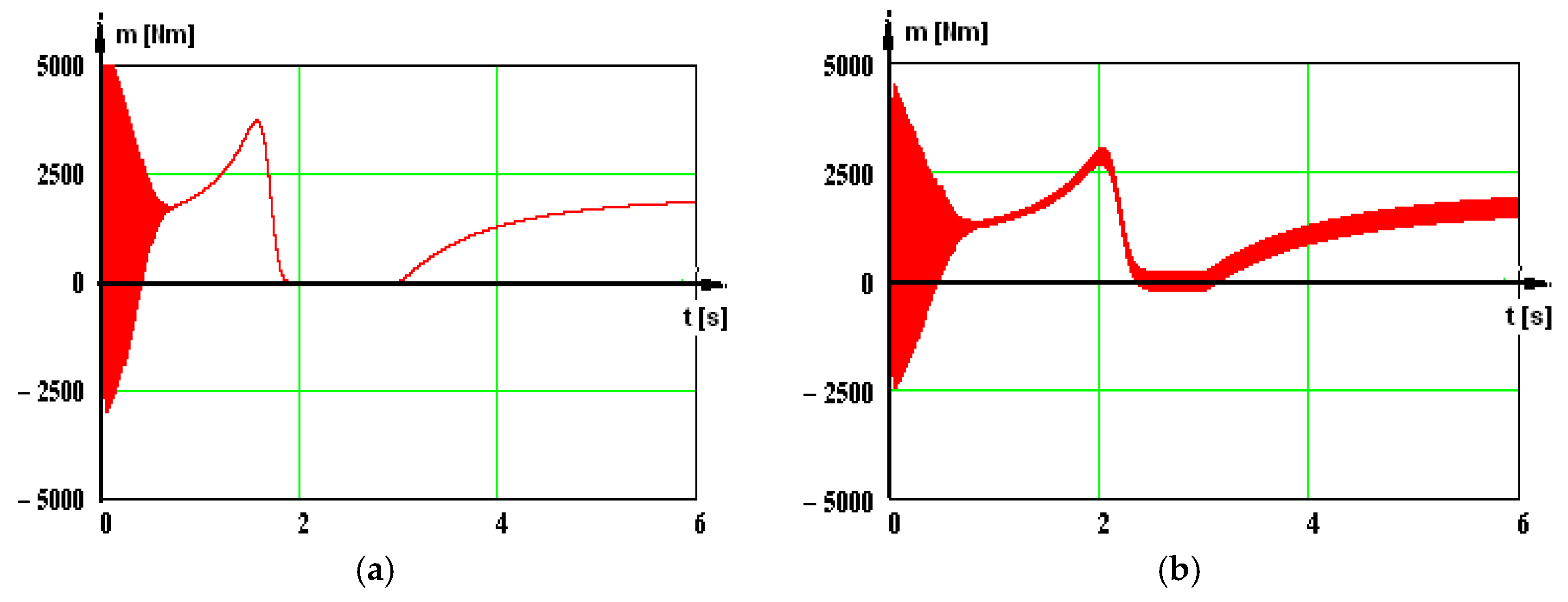
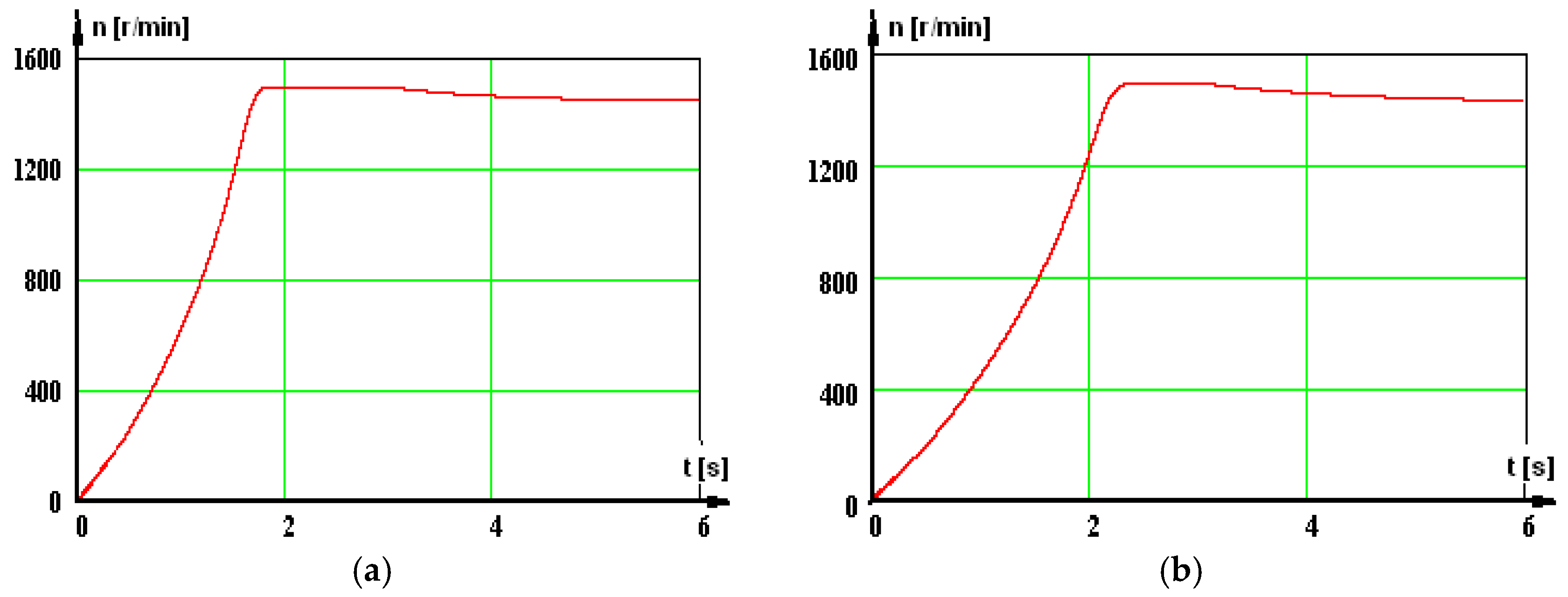
In the first moments of the dynamic regime, we noticed the curves of time variation of the phase currents (high amplitudes) (Figure 3) and the torque variation curves (high values) (Figure 4), which rapidly accelerate the rotor, causing a speed increase (Figure 5). In Figure 3, Figure 4 and Figure 5, there are curves presented for the two cases analyzed: network and static converters.

When the no-load operation is reached, the phase current and the torque are settled at low values, corresponding to the torque of the losses, M_st = 30 Nm (Figure 3 and Figure 4), and the speed obtains a no-load value (Figure 5). After that, the load is coupled, which, due to its high inertia moment, causes a new, long-lasting dynamic regime. The evolutions for the phase current, torque, and speed in this period are depicted in Figure 3, Figure 4 and Figure 5.

The quality of the simulations carried out also consists of the number of points used: N_pper = 399—number of points on a period of the input signal (phase voltage); N_per = 300—number of periods necessary for the dynamic regime. However, T₁ = 0.02 s—the signal period, results in t_p = N_per·T₁ = 6 s—the duration of the dynamic regime; N_p = N_per·N_pper = 119,700—the number of points for a quantity (voltage, current, torque, etc.).

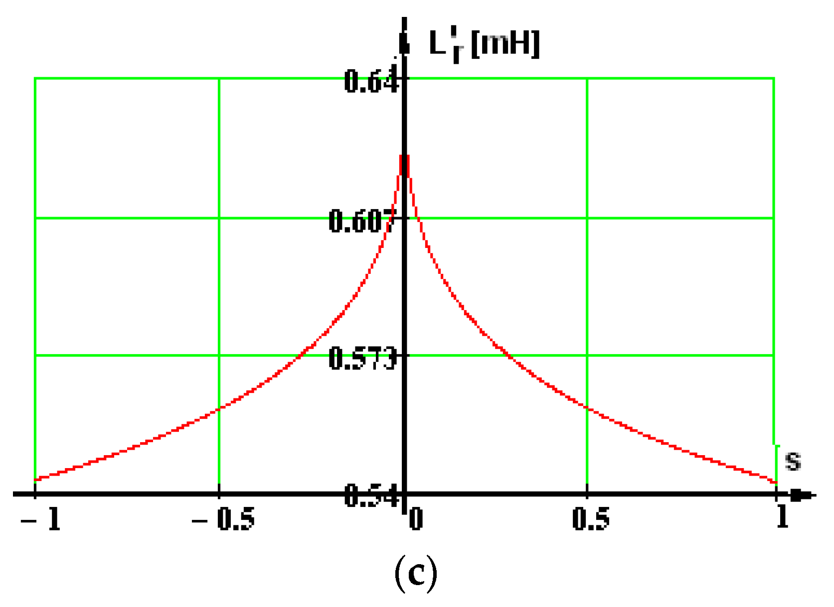
Using the data from the motor technical data sheet and a design program made by the authors, it was redesigned, and further, the parameter variation curves in relation to displacement and magnetic saturation were established. In fact, the two phenomena are dependent on a single variable, “n”—the speed.

When this variable changes, we have a variation in the frequency of the magnetic field in the rotor and, as a result, the effect of pushing back the current in the rotor bars, characterized by an increase in the resistance of the rotor bar and a decrease in inductance. The n-speed variable modifies the “s” slip, which changes the motor load and, therefore, the currents through the windings and therefore the magnetic saturation.

The computation relationships of the parameters affected by repulsion and magnetic saturation are given in the literature [7,8]. These relations are used, and the sliding in a wider interval is considered s (−1, 1). If N_s is the number of points in which the interval is divided, for the corresponding slips and the known relationships, the values of the parameters are computed: $R_r^{\prime }$—the resistance per phase of the rotor with repulsion, $L_s$/$L_r^{\prime }$—the reported stator and rotor inductances modified due to repulsion and magnetic saturation. The graphic representations for these parameters are given in Figure 6.

During the analyzed dynamic regime, the speed and the currents in the windings are variable, but known quantities are established by numerical computation. Using the previous curves, in relation to the motor speed determined by computation, the motor parameters are updated at each iteration in order to obtain the most accurate results.

The time variation curves of the parameters during the analyzed dynamic regime are as follows: Figure 7a—the curve of the variation in the reported resistance of the rotor $R_r^{\prime }$, Figure 7b,c—the variation curves of stator L_s and rotor inductances reported $L_r^{\prime }$.

In the case of supplying via a static converter, for the last period of the dynamic regime (Figure 8), the geometrical locus curves have been plotted for the following: i_s—stator current, i_r—rotor current, and i_1m—magnetization current.

3.2. Establishing the Root-Mean-Square (Average) Values during the Dynamic Regime

In order to increase the determinations precision, high inertia moments have been considered (for the starting and load) to obtain a long duration of the dynamic regime, so an important number of oscillations has been used for the current and for the torque.

For each oscillation of the current, the root-mean-square value has been computed (I_1r—network, I_1cs—static converter) using known numerical methods (8), thus resulting in the current curve (root-mean-square value) for the entire dynamic regime analyzed. Similarly, this has been performed for the supply phase voltage.

$$I{1}_k=\sqrt{{\displaystyle \frac{1}{T_1}}{\displaystyle \sum _{j=k·N_{pper}}^{(k+1)·N_{pper}}{\left(i{1}_j\right)}^2·h_t}}$$

(8)

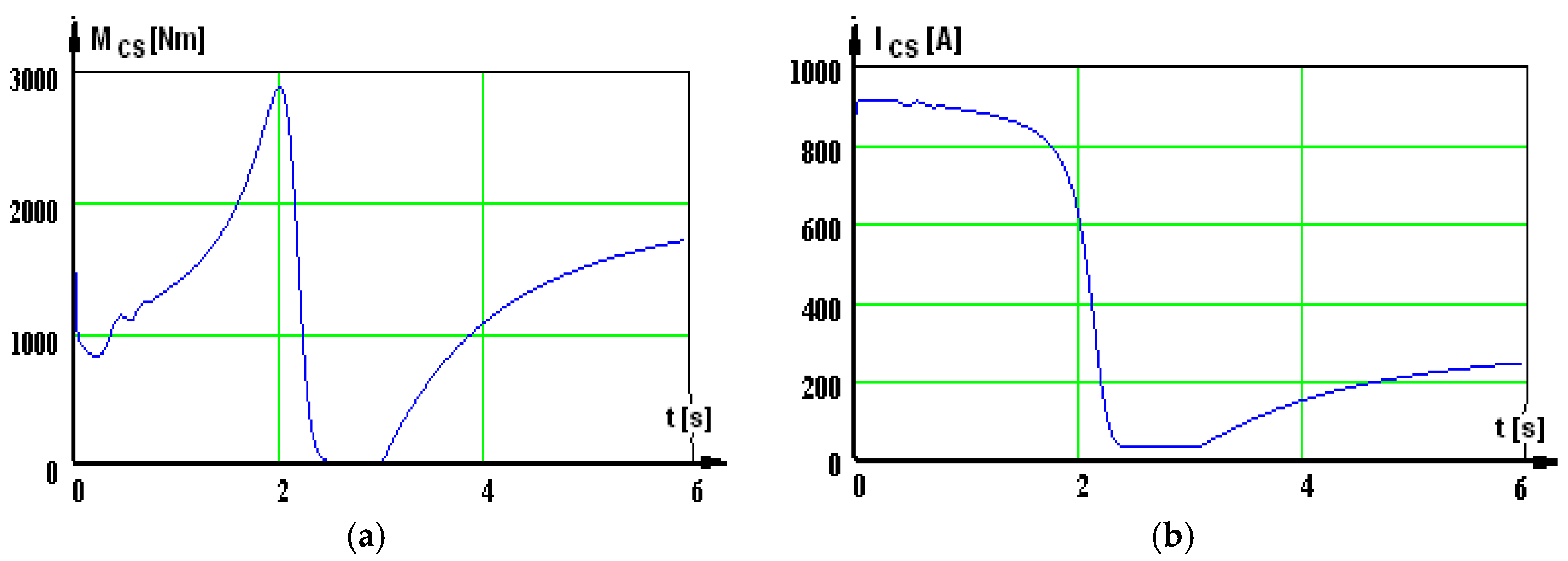
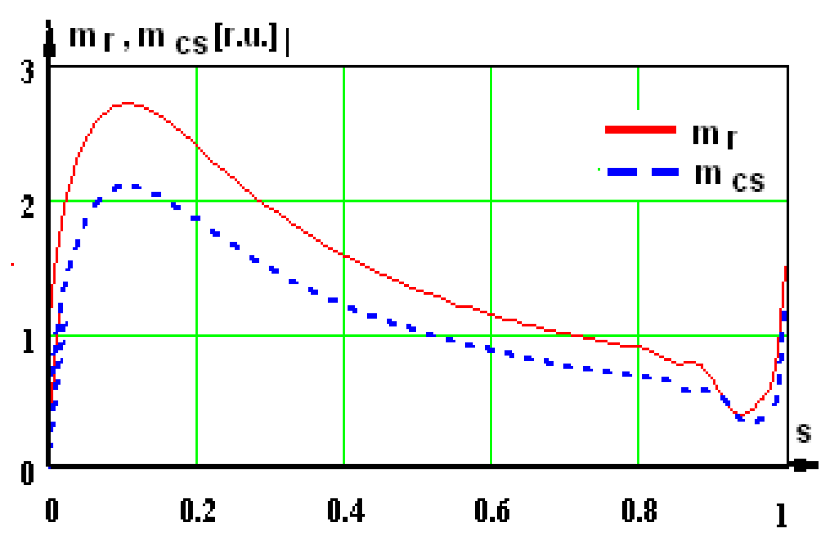
For each voltage period, regarding the torque variation curve (Figure 4a,b), its average value was calculated with relation (9) for the cases (M_r—network, M_cs—static converter). In this case, the number of points related to this curve is equal to the number of periods, N_f = N_per = 300.

$$M_k={\displaystyle \frac{1}{N_{pper}}}{\displaystyle \sum _{j=k·N_{pper}}^{(k+1)·N_{pper}} \left(m_j\right)}$$

(9)

M_k—the average value of the torque during a voltage oscillation period; N_pper—the number of points during a period; k—the number of the iteration period; m_j—the momentary value of the torque within the analyzed period.

Similarly, for the speed, it is noticed that, owing to the high inertia moment, the speed curve does not contain any oscillations. Consequently, the one from Figure 4 is valid.

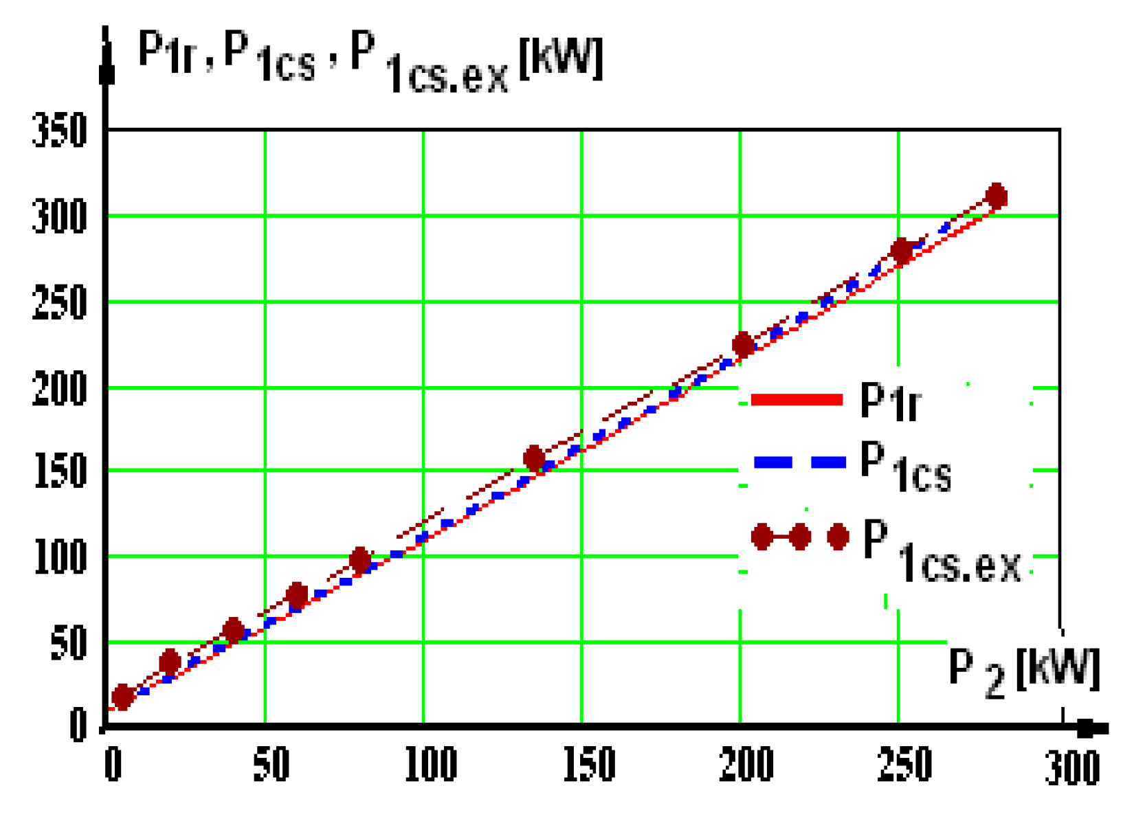
The active electrical power taken from the network (10) is the average value on each period of the instantaneous power (p₁ = u₁·i₁), and thus, the curves of the powers P_1r and P_1cs are a result.

$$P{1}_k={\displaystyle \frac{0.001}{N_{pper}}}{\displaystyle \sum _{j=k·N_{pper}}^{(k+1)·N_{pper}} \left(u_j·i_j\right)}$$

(10)

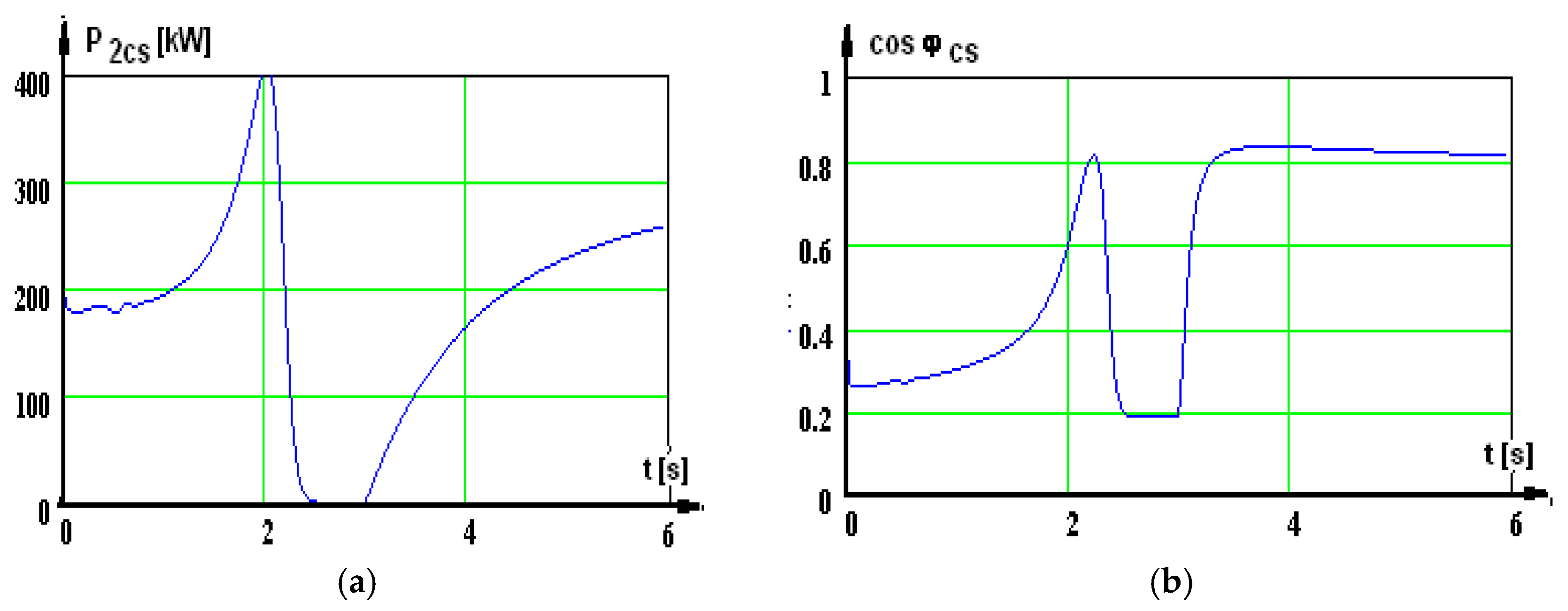
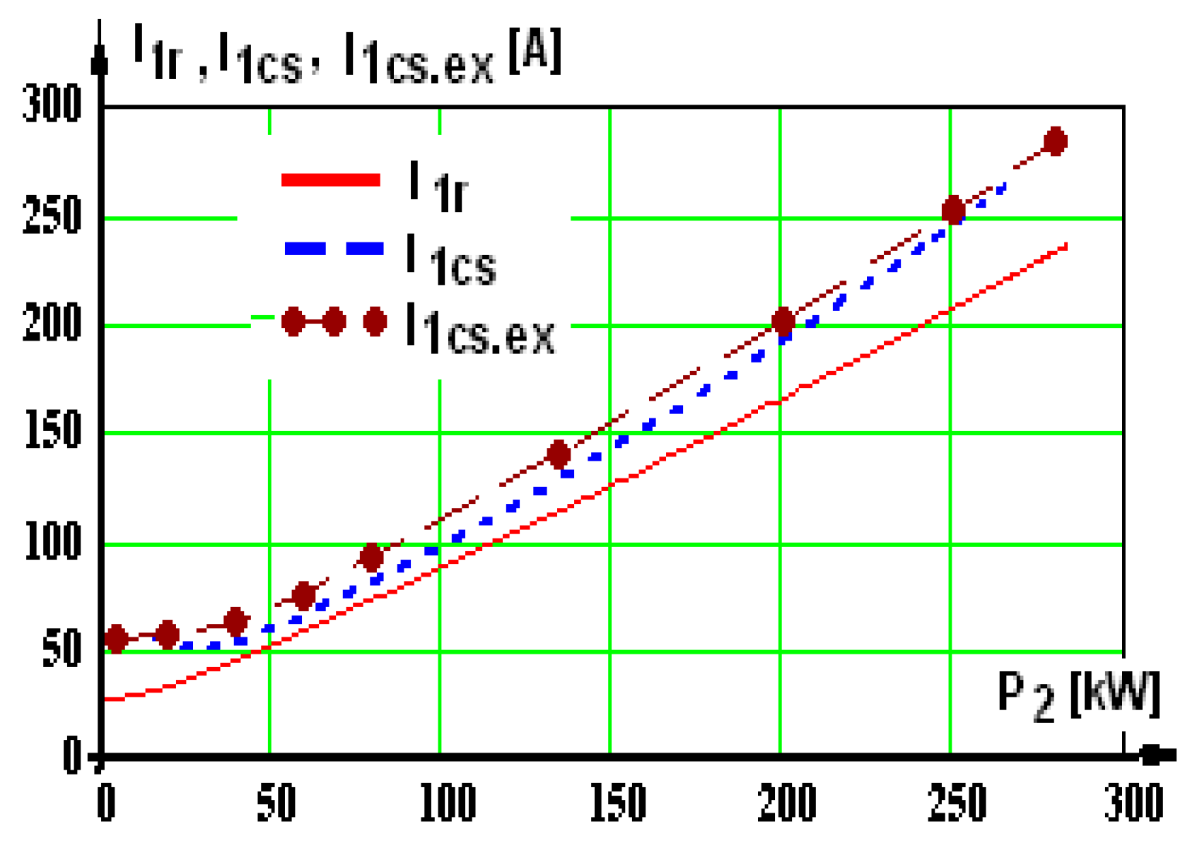
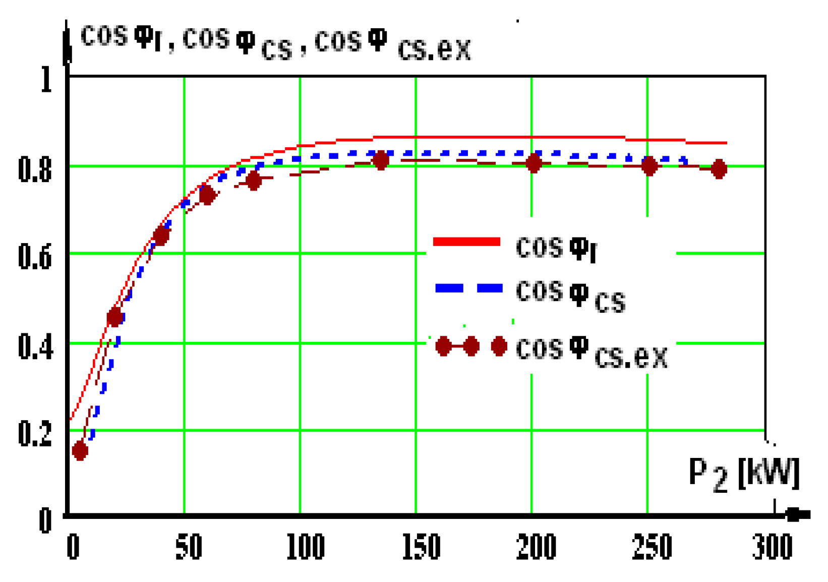
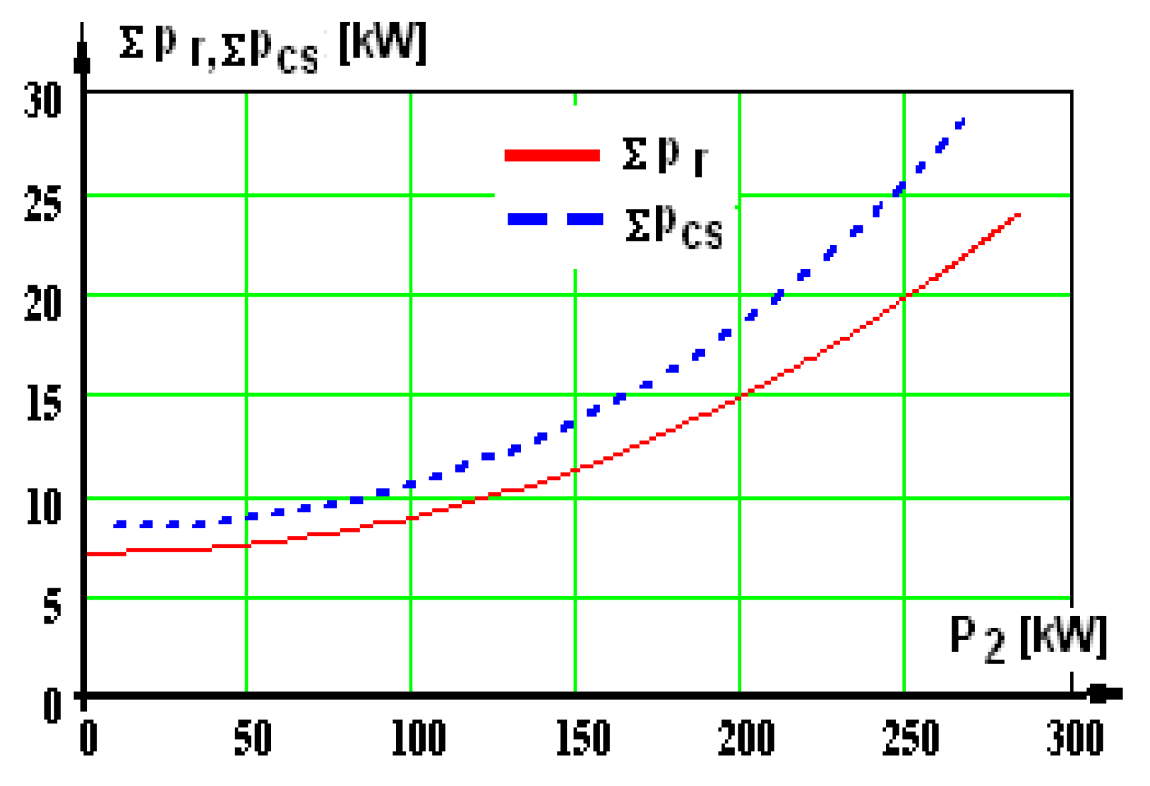
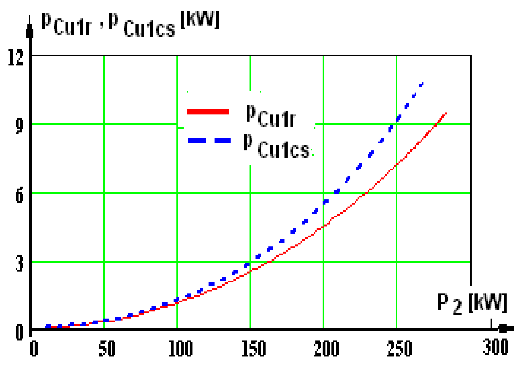
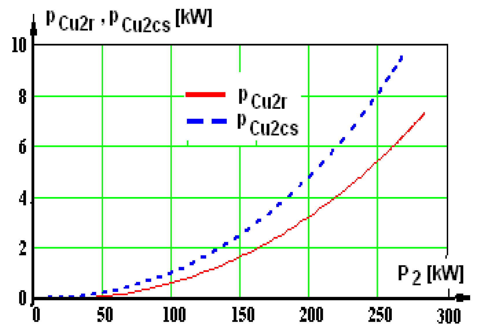
With these results, the losses are computed further on: losses in the machine Σ_pr and Σ_pcs, shaft useful mechanical power P_2r and P_2cs, efficiency η_r and η_cs, apparent power S_1r and S_1cs, reactive power Q_1r and Q_1cs, power factor cosφ_r and cosφ_cs, and graphic representations are plotted.

A few representative curves are presented further on: the shaft’s useful mechanical power (Figure 9a), current (Figure 9b), useful mechanical power (Figure 10a), and power factor (Figure 10b), corresponding to supplying via a static converter.

From space considerations, there is no presentation of either all curves obtained or the curves obtained in the case of supplying via the three-phase network.

4. Operation Characteristics of Asynchronous Motor in Steady Regime

The definitions of the operating characteristics are detailed in

Table 1. Definitions of operating characteristics.

Notations	Meanings
I1 = f(P2)	current characteristic
M = f(P2)	electromagnetic torque characteristic
cosφ = f(P2)	power factor characteristic
n = f(P2) or s = f(P2)	speed characteristic or slip characteristic
P1 = f(P2)/Q1 = f(P2)/S1 = f(P2)	input power characteristics active/reactive/apparent
η = f(P2)	efficiency characteristic
Σp = f(P2)	total losses characteristic
pCu1 = f(P2)/pCu2 = f(P2)	losses characteristics for stator winding/rotor winding
M = f(s).	natural mechanical characteristic, in p.u.

.

In the simulations presented before (Figure 9 and Figure 10), if the variable “t”—time—is removed, the known operation characteristics result.

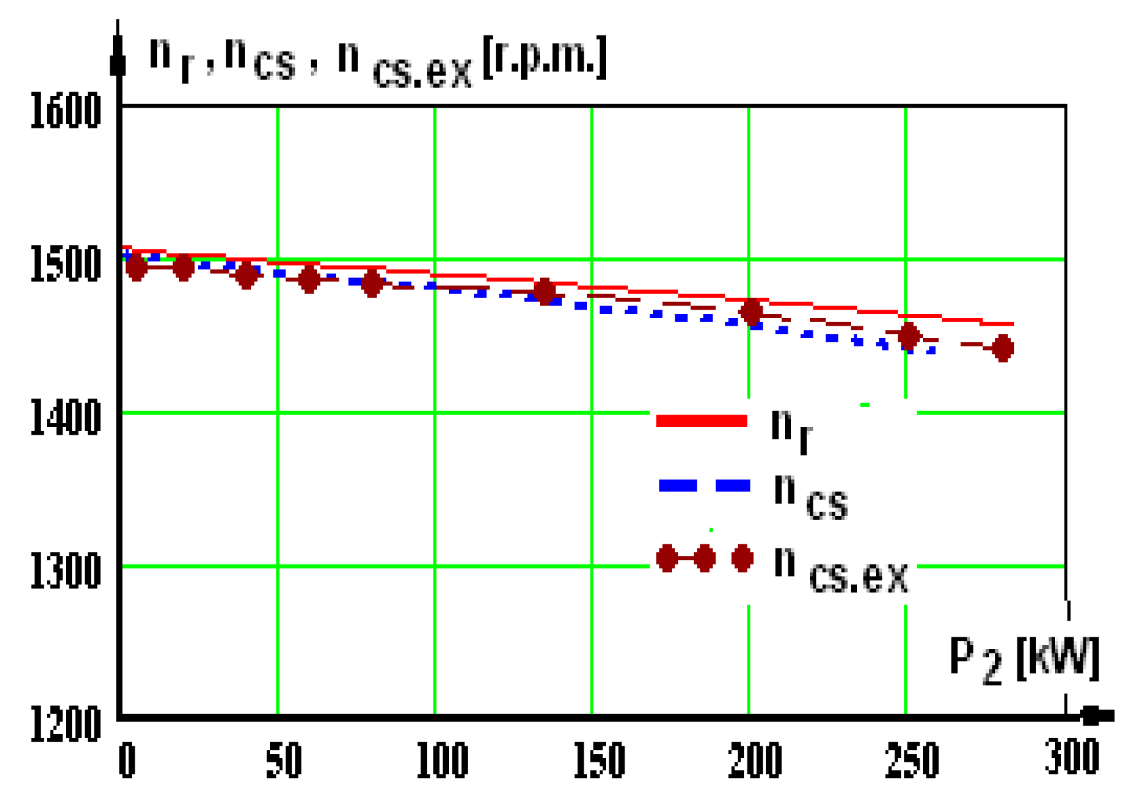
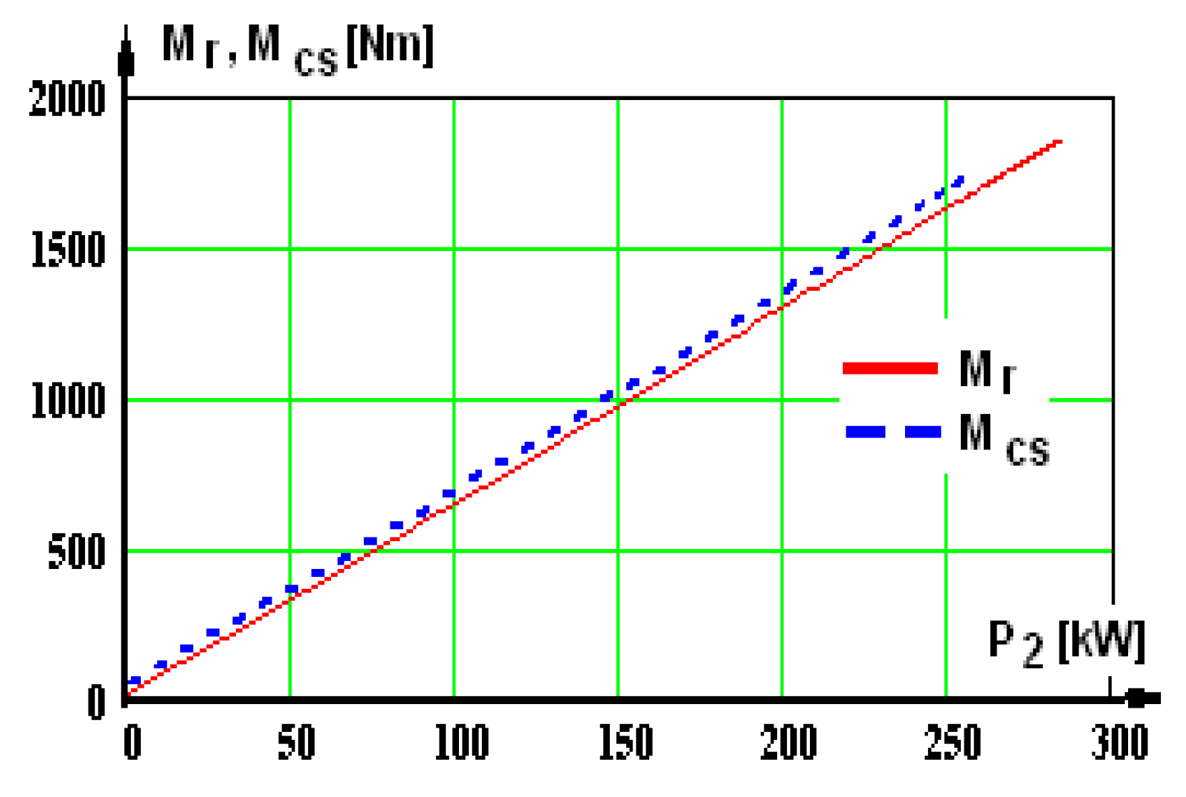
The characteristics previously presented obtained by simulation are plotted in Figure 11, Figure 12, Figure 13, Figure 14, Figure 15, Figure 16, Figure 17, Figure 18, Figure 19, Figure 20, Figure 21 and Figure 22. In these graphs, on the Ox axis, we have P₂—the mechanical power at the shaft. There are two curves in each graphic: one of them has the index “r”, afferent to supplying from the network, the second has the index “cs”, afferent to supplying from the static converter.

In some graphs, there is a third curve, marked with the index “ex”—experimental, obtained by testing the motor supplied by a static converter in a certified laboratory.

In the experimental part, the motor was powered by a static voltage and frequency converter with voltage U = 800 V and frequency f = 50 Hz and was loaded up to the nominal load, and at this interval, nine measurements were made.

When the voltage and frequency static converter are available, tests with the asynchronous motor will be carried out in order to verify the rated load operation. This way, the characteristics having the same name are placed in the same graphic and can be compared more easily. In the analysis of the graphics containing the experimental results as well, it is noticed that there are admissible differences between the simulated curves (noted with index “r”) and the experimental ones (noted with index “ex”). In the two cases, “r” and “ex”, the three-phase sinusoidal source has been used, U = 800 V and f = 50 Hz. The test of the operation of the asynchronous traction motor under load was carried out in an accredited testing laboratory, and a diagram of the power circuit in the recuperative system is shown in Figure 23 (the notations are detailed in

Table 2. The meanings of the notations used in Figure 23.

Notations	Menings
M.A.	asynchronous motor
G.S.	synchronous generator
M.A.T.	asynchronous traction motor
G.c.c.	D.C. generator with tilting pendulum-type stator that offers the possibility of measuring the mechanical torque from the shaft
M.c.c.	DC motor
M.A.R.	asynchronous motor working in asynchronous generator mode
KR, KM	switches
	contactor
Kcc	d.c. switch
T.G.	tachogenerator
T.M.	electronic three-phase measuring kit
T.C. IA, T.C. IB, T.C. IC	current transformers
T.U. UA, T.U. UB, T.U. UC, T.U. UTG	voltage transducers

).

The operating characteristics were established experimentally through nine points, with some by direct measurements and others by computation.

The results for the rated load, obtained by simulation, are presented in

Table 3. Results at nominal engine load: simulated and experimental.

Quantity Analyzed	Symbol	MU	Simulation of the Load Regime		Experimental Tests	Supply VFSC Tests- Simulation Error (%)
			Supply Three-Phase Network	Supply VFSC	Supply VFSC
Supply voltage	UN	V	800	800	800	-
Resistant torque	Mr	Nm	1635	1635	1633	-
Maximum torque	Mmax	Nm	2.28·MN	1.85·MN	1.89·MN	-
Phase stator current	I1	A	202.9	246.2	252.4	2.50
Speed	n0	r/min	1464	1444	1449	0.345
Useful mechanical power	P2	kW	250	250	250	-
Active power received from the supply network	P1	kW	269.15	275.6	277.2	0.577
Apparent power received	S1	kVA	289.9	324.1	336.7	3.70
Reactive power received from the supply network	Q1	kVAR	107.4	143.7	149.2	3.70
Power factor	cosφ		0.929	0.811	0.798	1.60
Efficiency	η		0.927	0.907	0.899	0.89
Total losses of the motor	Σp	kW	19.15	25.6	27.2	5.90
Stator winding losses	pCu1	kW	7.23	8.616	-	-
Rotor winding losses	pCu2	kW	5.39	6.548	-	-

for two cases: supply via the network and a static converter.

The experimental results were determined for the rated load and motor supplied via a converter. The voltage curve at the converter output (obtained with data acquisition) was used to obtain the simulations.

The simulation results for the power supply by the converter are presented in column 5, and the experimental results are presented in column 6. In column 7, the errors between the simulation and experiment (columns 5 and 6) are presented, computed using the following relation:

$$\Delta x(\%)=100·\left|{\displaystyle \frac{X_{simulare}-X_{ex}}{X_{ex}}}\right|$$

(11)

Higher differences occur in currents, 2.59%, with total loss of 5.492%, reactivity of 3.71%, and apparent powers reaching 3.68%.

In the analysis of these simulated curves (by supplying the three-phase network with a voltage and frequency static converter, respectively), it is noticed that certain differences occur, a fact justified by the presence of superior harmonics in the voltage and current curves.

Importantly, very high differences occur in the natural mechanical characteristics analyzed in the two situations. You can see a pronounced decrease in the critical torque with Δm = 27.2% (relative to the maximum torque), because the simulations were made for U_r = U_cs = 800 V (equal effective values of the network and converter voltages).

As a result, the fundamental voltage harmonic is smaller, and this is where the decrease comes from. The value of the maximum torque is an important quantity in electric traction.

By analyzing the table presented above, it can be noticed that

ΔΣp = Σ_pcs − Σp_r = 25.6 − 19.15 = 6.45 kW

There are higher losses in the traction motor in the case of supplying via the static converter compared to the sinusoidal regime for the rated load.

However, N_m = 6 is the number of motors, thus resulting in a significant increase in losses for a single locomotive:

ΔΣpt = N_m·ΔΣp = 6·6.45 = 38.7 kW

which is similar to the reactive power consumed:

ΔΣqt = N_m·(Q_1cs − Q_1r) = 6·(143.7 − 107.4) = 217.8 kVAR

So, the supply from the static converter means an increase in losses by 30.2% compared to the total losses, as well as an increase in the active power received from the network by 2.21%.

An estimative computation was carried out, starting with N_o = 10 h—average number of daily operation hours for a locomotive, N_z = 330 annual number of operation days, and T_ri = 15—time of the investment recovery.

On the basis of these data, extra energy active consumption results in

W_el.a = ΔΣpt·N_o·N_z·T_ri = 38.7·10·330·15 = 1916 MWh

with the following, respectively, for the reactive power consumed:

W_el.r = ΔΣqt·N_o·N_z·T_ri = 217.8·10·330·15 = 10,780 MVARh

4.1. Analysis of the Distorting Regime in Case of Supplying the Traction Motor from the Voltage and Frequency Static Converter

Further on, a harmonic analysis of the important quantities conditioning the traction motor operation is carried out, corresponding to supply via the static converter, in order to establish the distortion degree. Details about these quantities are given in Figure 24, Figure 25, Figure 26, Figure 27, Figure 28 and Figure 29.

4.1.1. Harmonic Analysis of the Supply Voltage

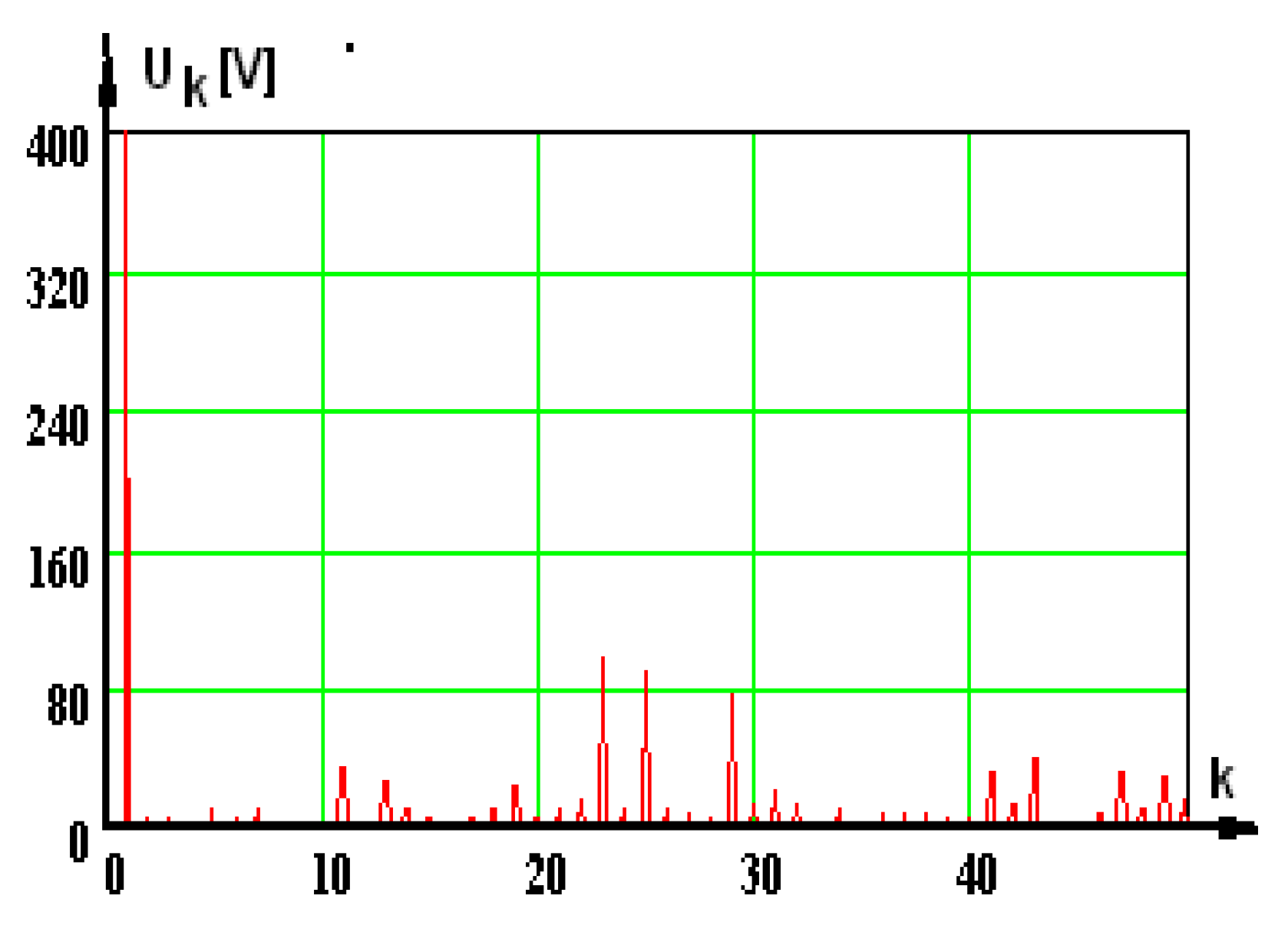
An important distortion degree of the supply voltage is noticed, caused by a high number of harmonics with important amplitudes. The affirmation is justified by k_dis.U = 41.14%—distortion factor.

Figure 24. The voltage values U_1cs—the phase voltage at the supply from the static converter; U_1,1cs—fundamental harmonic.

Figure 24. The voltage values U_1cs—the phase voltage at the supply from the static converter; U_1,1cs—fundamental harmonic.

Figure 25. Harmonic spectrum of the supply voltage (k—harmonic order).

Figure 25. Harmonic spectrum of the supply voltage (k—harmonic order).

4.1.2. Harmonic Analysis of the Motor Phase Current

It is noticed that there is a very low distortion degree of the current at the output of the static converter, which is caused by a small number of weightless harmonics. The affirmation is justified by k_dis.I = 7.704%—distortion factor.

Figure 26. The current values. I_1cs—the phase current at the supply from the static converter in stationary mode; I_1,1cs—its fundamental harmonic.

Figure 26. The current values. I_1cs—the phase current at the supply from the static converter in stationary mode; I_1,1cs—its fundamental harmonic.

Figure 27. Harmonic spectrum of the supply current (k—harmonic order).

Figure 27. Harmonic spectrum of the supply current (k—harmonic order).

4.1.3. Harmonic Analysis of the Electromagnetic Torque

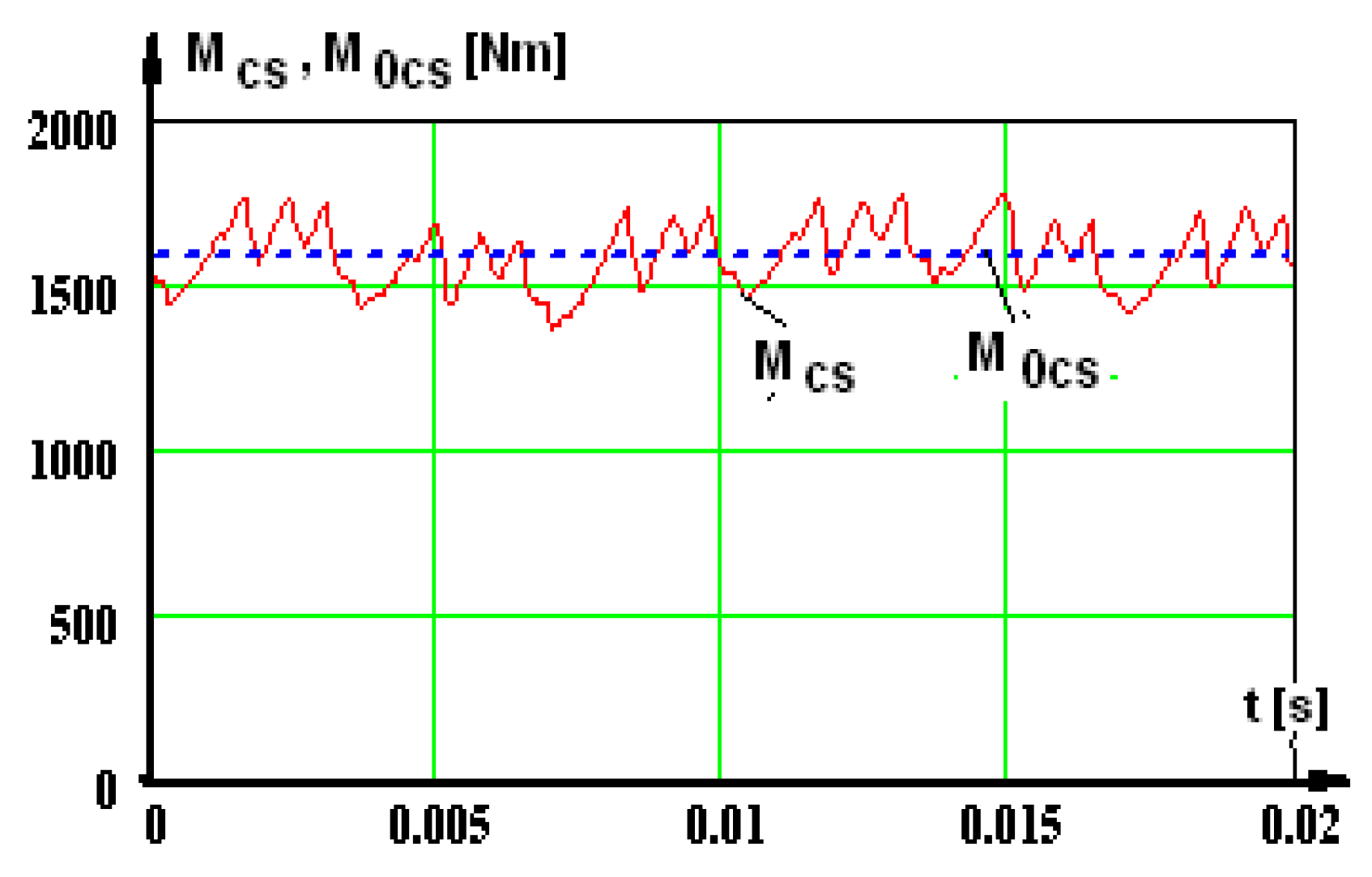
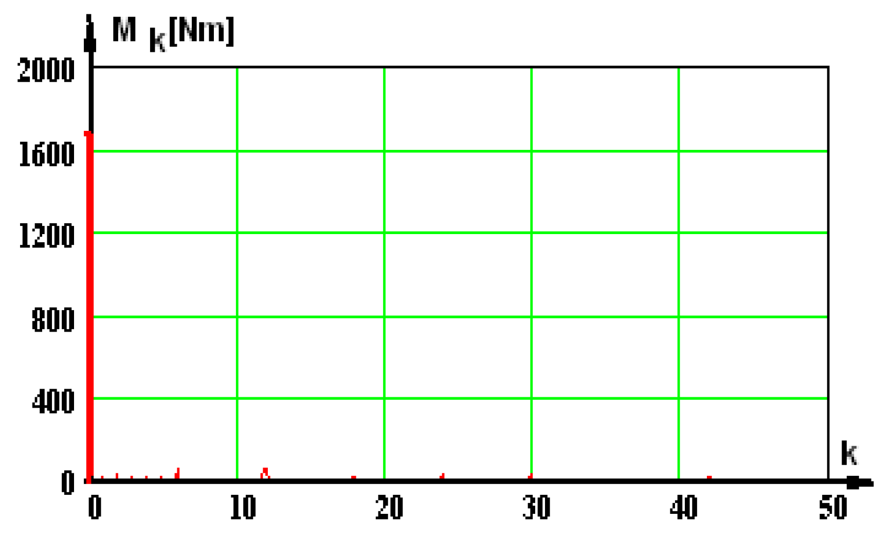
It is noticed that there is a very low distortion degree of the electromagnetic torque, which is caused by insignificant harmonics such as magnitude and amplitude. The affirmation is justified by k_dis.M = 5.67%—distortion factor.

Figure 28. The electromagnetic torque values. M_cs—the electromagnetic torque at the supply from the static converter in stationary mode; M_0cs—continuous component.

Figure 28. The electromagnetic torque values. M_cs—the electromagnetic torque at the supply from the static converter in stationary mode; M_0cs—continuous component.

Figure 29. Harmonic spectrum of the electromagnetic torque (k—harmonic order).

Figure 29. Harmonic spectrum of the electromagnetic torque (k—harmonic order).

4.1.4. Other Important Aspects of the Distorting Regime

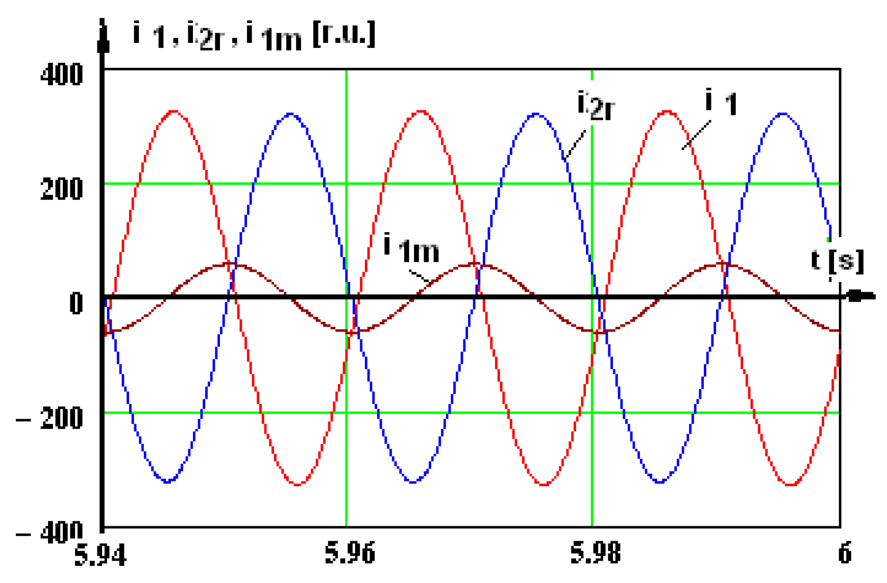
In the case of supplying via the three-phase source and in rated load, P_N = 250 kW, Figure 30 includes the plotted variation curves for the following: i₁—stator phase current, i_2r—rotor phase current in relative units, i_1m—magnetization current.

In Figure 31, we have the same curves, but in this case, the motor is supplied by a static converter. It is noticed that there is a sinusoidal magnetization in the two cases.

In the final part of the distorting regime analysis (Figure 32), we have the graphic with the three afferent curves: u—supply voltage; u₁/i₁—fundamental harmonics for voltage and current. It is possible to see the inductive character of the load produced by the voltage–current phase shift.

5. Conclusions

In the analysis of Figure 11, Figure 12, Figure 13, Figure 14, Figure 15, Figure 16, Figure 17 and Figure 18, we notice that, in the case of a three-phase sinusoidal power supply, we have small differences between the simulated curves and those determined experimentally.

This justifies definitively that the possibility of chaos arising from the solution of the system of coupled differential equations is very small.

The quality of the simulations and results presented must be noted, which enables us to extend the analysis to other types of traction motors, too, in order to establish whether they correspond to the exploitation requirements in order to increase sustainability.

The conclusion regarding the increased losses in the motor is as follows: the method of forming the voltage and the carrier frequency generates the harmonic distortions of the three-phase voltage supplied by the static converter of the asynchronous traction motor.

These results show us how the analyzed asynchronous traction motor behaves, from an energetic point of view, in operation.

The analysis of the stator phase current curve shows a small number of harmonics with no weight, the statement justified by k_dis.I = 9.23%—the distortion factor. These harmonics will also be found in the power supply network of the locomotives and determine a distorting regime and a decrease in the power factor.

Keeping the imposed rated data of the asynchronous motor, it can be redesigned and, based on the results obtained, new research is performed using the same static converter. In this way, after a wider activity, the optimal sustainable version of the asynchronous motor is obtained, which is fed from the imposed static converter, ensuring a more rational use of electricity.