Three-Dimensional Aerodynamics and Vortex-Shedding Characteristics of Wind Turbine Airfoils over 360-Degree Angles of Attack

Abstract

In this work, we present the first three-dimensional (3D) computational investigation of wind turbine airfoils over ${360}^{°}$ angles of attack to predict unsteady aerodynamic loads and vortex-shedding characteristics. To this end, static–airfoil simulations are performed for the FFA-W3 airfoil family at a Reynolds number of ${10}^7$ with the Improved Delayed Detached Eddy Simulation turbulence model. Aerodynamic forces reveal that the onset of boundary-layer instabilities and flow separation does not necessarily coincide with the onset of stall. In addition, a comparison with two-dimensional simulation data and flat plate theory extension of airfoil polars, suggest that, in the deep stall regime, 3D effects remain critical for predicting both the unsteady loads and the vortex-shedding dynamics. For all airfoils, the vortex-shedding frequencies are found to be inversely proportional to the wake width. In the case of slender airfoils, the frequencies are nearly independent of the airfoil thickness, and their corresponding Strouhal number $St$ is approximately $0.15$. Based on the calculated $St$, the potential for shedding frequencies to coincide with the natural frequencies of the International Energy Agency 15 MW reference wind turbine blades is investigated. The analysis shows that vortex-induced vibrations occur primarily at angles of attack of around $\pm {90}^{°}$ for all airfoils.

1. Introduction

With global offshore wind energy capacity expected to exceed 75 $\mathrm{G}$$\mathrm{W}$ in 2024 [1], larger machines with ratings between 11 $\mathrm{M}$$\mathrm{W}$ and 15 $\mathrm{M}$$\mathrm{W}$ are being deployed worldwide to help meet industry needs. As wind turbines become larger, the aerodynamic performance of their blades, including the individual airfoils, need to be reassessed. This is because an increased blade size introduces additional considerations and challenges, including the ability of existing models to predict phenomena associated with higher Reynolds numbers, as well as vortex-induced vibrations and three-dimensional (3D) flow separation at high, post-stall angles of attack, and $\alpha$ [2]. To this day, numerous wind tunnel tests have been conducted to investigate the aerodynamic performance of wind turbine airfoils [3,4,5,6]. These studies were instrumental in providing vital information regarding the lift, drag, and moment coefficients of wind turbine airfoils under normal operation ($\left|\alpha \right|<$ 20°), as well as at a Reynolds number on the order of ${10}^6$. The present work aims at numerically reassessing the aerodynamic coefficients of airfoils relevant to offshore wind turbines both over 360° angles of attack and at a higher Reynolds number: $Re={10}^7$. Due to the paucity of publicly available data from commercial blade airfoils, for this study, we have selected the nonsymmetric Flygtekniska Försöksanstalten Aeronautical Research Institute of Sweden (FFA) [7] airfoil family. The FFA airfoil family, while not fully representative of modern turbine airfoils, is amongst the most well-documented datasets, with some experimental data also being available for validation [6]. As such, the family has become increasingly popular within the wind energy research community and has been used in many reference turbines such as the International Energy Agency (IEA) Wind 10 MW [8], 15 MW [9], and 22 MW [10]. In this study, the adoption of the FFA-W3 family aligns with contemporary practices, aiming to furnish essential insights for design engineers and researchers.

Wind turbine blades are routinely subjected to high wind speeds and intense turbulence. Under these conditions, the effective angles of attack, ${\alpha }_{\mathrm{eff}}$, at multiple radial locations along a blade’s span can become large enough to trigger massive flow separation. In this flow regime, also known as the deep stall regime, the separated shear layer rolls up to form highly energetic vortices. These, in turn, cause strong boundary-layer separation and reattachment. As a result, the blades can experience significant levels of unsteady loading. Moreover, under extreme wind conditions, the turbines are put in shutdown mode with their blades feathered to ${90}^{°}$ in an attempt to generate limited rotor torque. In this configuration, known as “idling”, ${\alpha }_{\mathrm{eff}}$ can reach $\pm {90}^{°}$ when experiencing a high mean yaw angle [11]. Consequently, the modern horizontal axis wind turbines fitted with large and flexible blades are susceptible to aeroelastic excitation, such as stall-induced vibrations (SIVs) and vortex-induced vibrations (VIVs). These phenomena occur when the vortex-shedding frequency of a blade approaches its natural frequency, resulting in large vibration amplitudes of the blade structure, which can trigger blade fatigue or even structural failure. A wide range of technologies for use in the flow control devices have been proposed in order to identify and damp the nonlinear vibrations [12].

Prior work in the literature includes studies of the Darrieus vertical axis wind turbine, where $\alpha$ approaches ${180}^{°}$ for low tip–speed ratios and operates at negative $\alpha$ as the blades rotate about the vertical axis [13]. In their study, Sheldahl and Klimas reported experimental data for the aerodynamic performance of NACA airfoils for $0^{°}\le \alpha \le {180}^{°}$ and Reynolds numbers ($Re$) ranging from ${10}^4$ to ${10}^7$. Similarly, Swalwell et al. [14] performed experiments on the NACA 0021 airfoil at $Re=2\times {10}^5$ to investigate the vortex-shedding frequency characteristics in the post-stall region. The study showed the frequencies based on both the lift and drag coefficients decline with an increase angle of attack; however, the Strouhal number ($St$), which is calculated based on the chord length normal to the freestream, remained nearly the same for all angles of attack when the flow was fully separated. In general, the airfoils considered in both the experimental studies are symmetric, where the magnitude of polars at negative $\alpha$ are identical to those at positive $\alpha$. However, wind turbine airfoils are typically nonsymmetric, and as such, their performance outcomes in deep stall and across all $\alpha$ values have not yet been investigated experimentally. The only experimental data available in the literature are for the FFA-W3-211 airfoil [15] at $Re=1.8\times {10}^6$, as well as FFA-W3-241 and FFA-W3-301 airfoils [6] at $Re=1.5\times {10}^6$. For all three airfoils, experiments were performed for $\alpha$ values between $0^{°}$ and ${20}^{°}$. This was well before the onset of the deep stall regime.

For the aviation airfoils, previous studies have demonstrated flat plate characteristics in the deep stall regime [16,17,18]. In general, the flow past an inclined flat plate has been extensively studied due to its wide range of practical engineering applications. Fage and Johansen [19] performed experiments at $\alpha$ values between ${12}^{°}$ and ${90}^{°}$ and showed that the shedding frequency decreased with an increase in the $\alpha$ value; however, the $St$ post $\alpha ={30}^{°}$ values remained approximately constant at $0.15$. Experiments by Chen and Yang [20] for flat plates with different beveled edges and for $\alpha$ values between $0^{°}$ and ${90}^{°}$, and $Re$ ranging from $3.5\times {10}^3$ to $3.2\times {10}^4$ also showed the frequency decrease. Furthermore, the frequencies at high $\alpha$ values were found to be independent of $Re$. The other well-known representative of bluff body flows is the circular cylinder. Flow past cylinders is of interest in the wind energy community due to the aerodynamics of the cylindrical shape blade sections at the blade root, as well as the aerodynamics of supporting structures, such as towers, monopiles, and certain parts of floating platforms. The effect of varying $Re$ between $2.3\times {10}^4$ and $7.1\times {10}^6$ on the mean and unsteady force coefficients, as well as the $St$, was investigated experimentally by Schewe [21]. The wakes behind bluff bodies have also been extensively investigated. Fage and Johansen [22] studied the vortex sheets in the wakes of several bluff bodies, including airfoils. The authors observed that the velocity distribution and the spread of turbulence in the sheets are highly dependent on the shape of the bluff body. Roshko [23], based on a semiemperical method, demonstrated that bluffer bodies tend to create wider wakes and that the wake width is inversely proportional to $St$.

With respect to vortex shedding, computational investigations of separated flows past bluff bodies, including aviation airfoils, have provided detailed insights into the mechanisms of flow separation across a wide range of operating conditions, which are otherwise difficult to obtain experimentally. Najjar and Vanka [24] performed 3D Direct Numerical Simulations (DNSs) of a flat plate held normal to the freestream at $Re=1000$ to study the 3D intrinsic instabilities. Resolving the instabilities was found to be crucial to correctly predict the mean and low-frequency variation of the drag coefficients ($C_d$) and to capture “rib-like” structures in the wake region. In the DNS study of a flat plate in deep stall, ref. [25] secondary instabilities present in 3D simulations generated smaller wake widths and lower $C_d$ than the corresponding two-dimensional (2D) simulations. For flow past cylinders, Mittal et al. [26] traced the overprediction of $C_d$ in 2D flows to higher $Re$ stresses in the wake.

The prohibitively high cost of DNS has restricted the method to low Re canonical flows. Alternately, Large Eddy Simulation (LES) methods, which model the computationally expensive smaller eddies, are also limited to low and moderate $Re$ flows. Therefore, Reynolds-averaged Navier–Stokes (RANS)-based methods, which model all turbulent scales, are still popular for a wide range of engineering applications; however, RANS models perform poorly for unsteady separated flows [18]. Hence, computational investigations of high-$Re$ massively separated flows have heavily relied on hybrid RANS/LES methods. The most popular are the family of eddy-resolving Detached Eddy Simulation (DES) methods. Originally developed by Spalart, ref. [27] the attached regions of the boundary layer are treated using a RANS model, and they only switch to the LES mode in the separated regions of the flow. Strelets [17] successfully demonstrated the method’s ability to accurately capture 3D-separated flows past NACA 0012 airfoils, circular cylinders, and landing gear trucks; however, the method is prone to model stress depletion, which causes spurious grid-induced separation and a log-layer match. Spalart et al. [28] proposed a model called Delayed Detached Eddy Simulation (DDES), which addressed the problem of model stress depletion by delaying the transition to the LES mode inside the boundary layer. Subsequently, Shur et al. [29] developed the Improved Delayed Detached Eddy Simulation (IDDES), which resolved both of the issues. Squires et al. [30] performed DES and DDES simulations of flow past a circular cylinder at $Re=8\times {10}^6$. The forces obtained with both models showed reasonable agreement with the experimental results [23]. Recently, Bidadi et al. [18] performed 3D computational investigations to study the effects of mesh resolution and IDDES turbulence models on the deep stall aerodynamics of NACA 0012 and 0021 airfoils at $Re=2.0\times {10}^5$ and $2.0\times {10}^6$. The authors showed that the IDDES model, together with appropriate spanwise mesh resolution, successfully captures both the deep stall aerodynamic coefficients, as well as the vortex-shedding frequency characteristics.

A large number of aerodynamic investigations in the literature have also focused on the linear and stall regions where the flow is not fully separated [9,31,32]. In the case of wind turbine airfoils, studies at high $\alpha$ values have so far focused on 2D flows. Bertagnolio et al. [32] conducted 2D simulations with a transition model for $\alpha <{30}^{°}$ of several wind turbine and NACA airfoils and compared the results with experiments and the XFOIL panel method data [31]. More recently, Gaertner et al. [9] conducted a 2D investigation of several FFA-W3 airfoils and $\alpha$ values between $-{180}^{°}$ and ${180}^{°}$. But, wind turbine airfoils are strongly influenced by 3D effects, such as boundary-layer separation and attachment, as well as vortex shedding from both the leading and trailing edges. The lack of resolving the 3D effects explains the absence of secondary peaks in the lift coefficients in deep stall. Therefore, in this work, for the first time, a 3D computational investigation was performed for seven FFA-W3 airfoils between $21\%$ and $50\%$ thickness with the IDDES hybrid RANS/LES turbulence model. For each airfoil, simulations were carried out for 59 angles of attack ranging from $-{180}^{°}$ to ${180}^{°}$. The aerodynamic polars generated from the static–airfoil simulation results were utilized to gain detailed insights into the impact of the nonsymmetric nature of the airfoils on the onset of 3D boundary-layer instabilities and stall. In the deep stall, the effects of varying the airfoil thickness and $\alpha$ values on the unsteady loads, vortex-shedding dynamics, and wake width were investigated. Subsequently, for each airfoil, the consequences of shear layer instabilities and flow separation on the amplitude of load oscillations, vortex-shedding frequencies, and Strouhal number ($St$) were discussed. Based on the frequency analysis, VIV lock-in regions onboard the IEA Wind 15 MW turbine blade were identified for airfoils operating at several wind speeds and $\alpha$ values.

The remainder of this paper is organized as follows. Section 2 discusses the governing equations and the discretization methods. Section 3 presents the problem setup, the simulation settings, and the meshing methodology. Section 4 discusses the effect of airfoil thickness on the aerodynamic loads, the vortex-shedding frequency characteristics, and the lock-in regions for the onset of the VIVs. Finally, Section 5 summarizes the main findings of this work.

2. Governing Equations and Discretization

The flow solver chosen for the present work is Nalu-Wind [33] (version 2.0.0), an open-source, unstructured grid, computational fluid dynamics solver designed for wind energy applications that is part of the ExaWind solver suite [34]. Nalu-Wind solves the incompressible form of the Navier-Stokes equations:

$$\begin{array}{cc}\hfill \mathrm{Continuity}\hspace{1em}\hspace{1em}\hspace{1em}\hspace{1em}\hspace{1em}\hspace{1em}\hspace{1em}\hspace{1em}\hfill & \hfill \hspace{1em}{\displaystyle \frac{\partial u_i}{\partial x_i}}=0,\end{array}$$

(1)

$$\begin{array}{cc}\hfill \mathrm{Momentum}\hfill & \hfill \hspace{1em}\hspace{1em}\rho {\displaystyle \frac{\partial u_i}{\partial t}}+\rho u_j{\displaystyle \frac{\partial u_i}{\partial x_j}}-{\displaystyle \frac{\partial \sigma }{\partial x_i}}=-{\displaystyle \frac{\partial p}{\partial x_i}},\end{array}$$

(2)

where $u_i$, p, and $\rho$ are the mean velocity in the $i^{th}$ direction, modified mean pressure, and density of the fluid, respectively. The equations are discretized using the second-order, node-centered, finite-volume method. Peclet blending and the implicit second-order backward difference scheme are used for advection stabilization and temporal discretization, respectively. For each time step solve, the time stepping algorithm consists of four Picard iterations. For each iteration, the momentum, Poisson pressure, and turbulence equations are solved. Next, the pressure projection algorithm is employed to calculate a divergence-free velocity field. For turbulent simulations, the diagonal portion of the advection and viscous terms are under-relaxed with the factor $\eta$ to improve the diagonal dominance of the linear system of equations. For the momentum and scalar equations, $\eta =0.7$, whereas for the pressure solve, $\eta =0.3$. Explicit relaxation of the variables are also performed using the same relaxation factors. The linear systems for all the equations are solved using the Generalized Minimal Residuals (GMRESs) iterative solver with the boomer Algebraic Multigrid (AMG) preconditioner in the Hypre library (version 2.31.0) [35]. For more details on the Nalu-Wind discretization and the use of linear solvers, the reader is referred to the papers by Domino [36] and Sharma et al. [37]. Turbulence is modeled with the IDDES hybrid RANS/LES method [38], which is based on the k-$\omega$ Shear–Stress (SST) model [39]. It solves equations for k and the specific dissipation rate $\omega$. In the RANS mode, k represents the total turbulent kinetic energy of the mean flow, whereas in the LES regions, k is a combination of total and sub-filter scale turbulent kinetic energy. The equations for k and $\omega$ are as follows:

$$\begin{array}{cc}\hfill {\displaystyle \frac{\partial k}{\partial t}}+U_j{\displaystyle \frac{\partial k}{\partial x_j}}\hfill & \hfill ={\displaystyle \frac{\partial }{\partial x_j}}\left(({\sigma }_k{\nu }_t+\nu ){\displaystyle \frac{\partial k}{\partial x_j}}\right)+\min \left(2{\nu }_t{S}_{ij}{S}_{ij},10{\beta }^{*}k\omega \right)-{\displaystyle \frac{\sqrt{k^3}}{l_d}},\hfill \\ \hfill {\displaystyle \frac{\partial \omega }{\partial t}}+U_j{\displaystyle \frac{\partial \omega }{\partial x_j}}\hfill & \hfill ={\displaystyle \frac{\partial }{\partial x_j}}\left(({\sigma }_{\omega }{\nu }_t+\nu ){\displaystyle \frac{\partial \omega }{\partial x_j}}\right)+{\displaystyle \frac{\alpha }{{\nu }_t}}\min \left(2{\nu }_t{S}_{ij}{S}_{ij},10{\beta }^{*}k\omega \right)\hfill \end{array}$$

(3)

$$\begin{array}{cc}\hfill \hfill & \hfill -\beta {\omega }^2+2{\sigma }_{\omega }{\displaystyle \frac{1-F_1}{\omega }}{\displaystyle \frac{\partial k}{\partial x_j}}{\displaystyle \frac{\partial \omega }{\partial x_j}},\hfill \end{array}$$

(4)

$$\begin{array}{cc}\hfill {\nu }_t\hfill & \hfill ={\displaystyle \frac{a_{1}k}{\max (a_1\omega ,2F_2{S}_{ij}{S}_{ij})}}.\hfill \end{array}$$

(5)

where $S_{ij}$ is the strain rate tensor, and $l_d$ is the destruction length scale, which is different for SST and IDDES models. The details on the constants and functions, ${\sigma }_k$, $F_1$, $F_2$, $a_1$, $\beta$, and ${\beta }^{*}$, can be found in [38,39].

3. Computational Setup

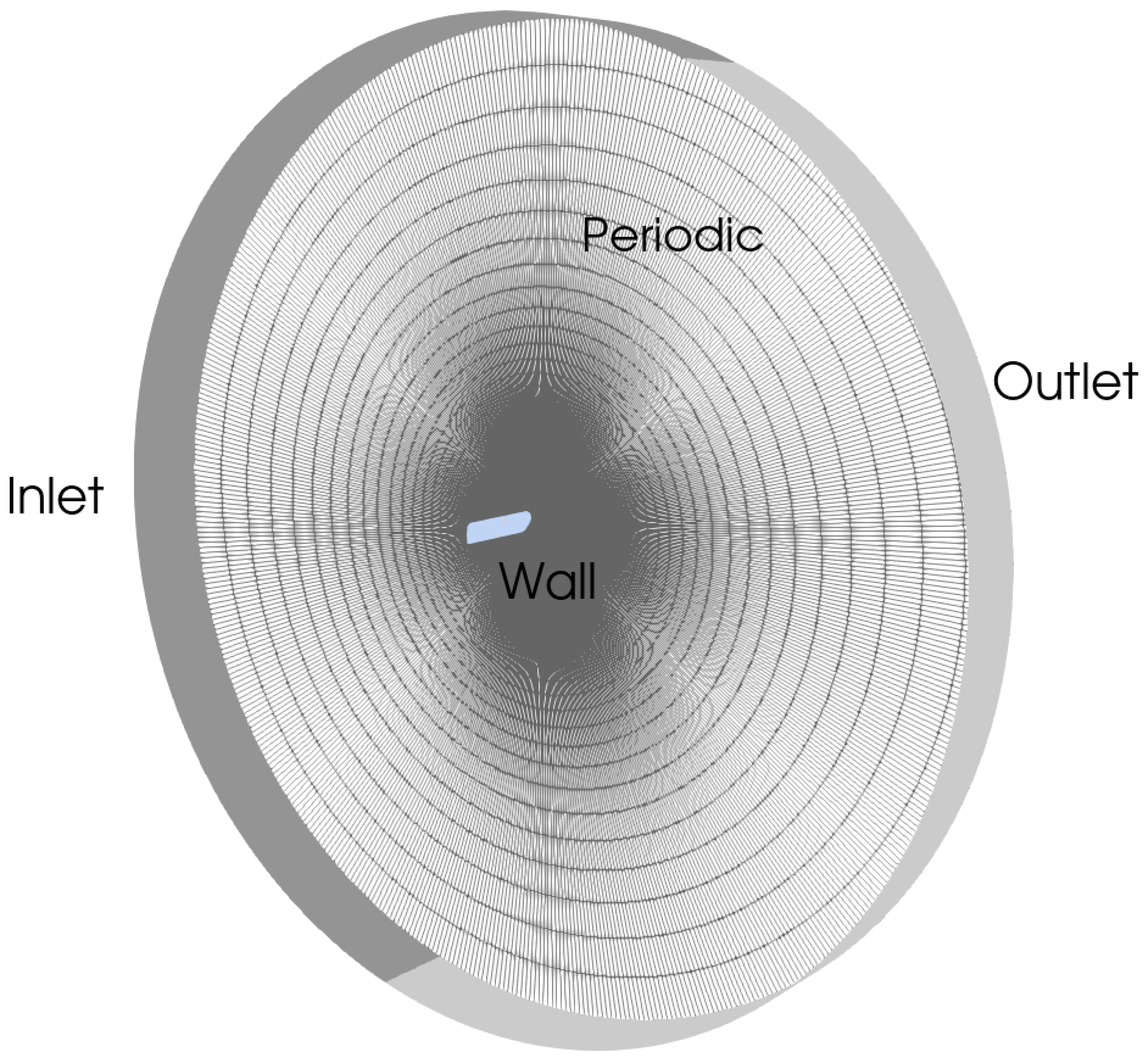
The computational domain, shown in Figure 1, consists of an O-grid, which extends 60 chord lengths, c, in the radial (x–y) directions and 4 chord lengths in the spanwise (z) direction. Roughly half of the outer boundary surface is treated as a velocity inlet, and the rest is treated as a zero-pressure outlet. The remaining boundary conditions are the no-slip wall on the bluff body’s surface, which is located at the center of the domain, and the translational periodicity in the z direction. The boundary conditions and their values are listed in

Table 1. Boundary conditions used in the simulations.

Region	Boundary Condition
Inflow	Velocity Inlet, $u_{inlet}=75$ m/s
Outflow	Pressure Outlet, $P_{outlet}=0$ Pa
Front/Back	Periodic Boundaries
Bluff body surface	No-Slip Wall, ${\mathbf{u}}_{wall}=0$ m/s

. Simulations were performed for all seven FFA-W3 airfoils, as well as the circular cylinder and the flat plate with the freestream velocity $u_{\infty }=$ 75 m s⁻¹, density ${\rho }_{\infty }=$ 1.2 kg/m³, and Reynolds number $Re={10}^7$. In all the simulations, the freestream turbulence was less than $0.05\%$, which is sufficiently small to not affect the aerodynamic load predictions.

Table 2. Physical properties of the flow.

Fluid Property	Value
Velocity	$u_{\infty }=75$ m/s
Density	${\rho }_{\infty }=1.2$ kg/m3
Reynolds number	$Re={10}^7$
Turbulent intensity	TI $<0.05\%$

presents the physical properties of the flow considered in the study.

Figure 2 shows 2D cross-section of the airfoils, the flat plate, and the circular cylinder. The flat plate has a thickness-to-chord ratio of $t/c=$0.02, with the radius of the rounded corners set to $0.01c$. Tian et al. [40] performed a LES study of a normal flat plate at $Re=1.5\times {10}^5$ for the radii of curvature $0.01c$ and $0.005c$ and showed that the smaller radius increased both the mean and fluctuations in the drag, as well as the complexity, of the flow downstream. Hence, a curvature of $0.01c$ has been chosen for the current study. Figure 3 presents the 3D meshes generated for FFA-W3-211, FFA-W3-500, and the flat plate at $\alpha =$ 32° and the circular cylinder. All grids were generated using a modified Pointwise glyph script [41]. The input parameters to the script include the first cell height, $\alpha$, the number of grid points in the chord and spanwise directions, and the cell growth rates in the wall normal direction. Two additional sets of parameters were specified to increase the mesh density near the leading and trailing edges. For all the runs, the first cell height based on $Re$ came out to 2.78 × 10⁻⁶ m, which corresponds to a wall distance of $y^{+}=1$. The number of cells per chord length in the spanwise direction was chosen to be 30. In the wall-normal direction, for accurate control of the mesh spacing near and away from the bluff body surface, a near-wall growth factor (NWGF) of $1.04$ and an off-wall growth factor (OWGF) of $1.09$ were chosen, which correspond to 288 wall-normal points. The number of spanwise and wall-normal points selected were based on our previous study on the NACA airfoils [18]. In the study, a comprehensive investigation on the effect of spanwise and wall-normal mesh resolutions combined with the k-$\omega$ SST RANS and IDDES hybrid RANS/LES turbulence model was performed. The spanwise mesh resolution investigated were 10, 24, and 30 cells per chord length, whereas in the wall-normal direction, 103, 143, and 251 points were chosen. This corresponds to NWGF and OWGF values of $1.12$ and $1.2$, $1.08$ and $1.15$, and $1.04$ and $1.09$, respectively. In the chordwise direction, nearly 250 points were chosen. The results of the aerodynamic polars and frequency analysis in deep stall show that a minimum of 24 cells per chord length in the spanwise direction, combined with 143 wall-normal points corresponding to NWGF and OWGF of $1.08$ and $1.15$, are necessary to obtain excellent agreement with the experimental results [13,14]. In this study, the wall-normal and spanwise grid resolution were finer than what is recommended in our previous study.

To determine the appropriate chordwise resolution, mesh resolution studies were performed for the FFA-W3-500 airfoil with 325, 525, and 725 chordwise points. The percentage differences in the lift and drag coefficients were compared for $\alpha$ values within the range ($\pm {30}^{°}$, $\pm {90}^{°}$). The wall-normal and spanwise resolutions were fixed at 288 and 121 points, respectively. The results show that the average percentage difference in the aerodynamic forces between the 325 and 725 meshes was greater than $8\%$, whereas the difference dropped to less than $2\%$ between the 525 and 725 meshes. Based on this study, and to minimize the computational cost, a resolution of 525 chordwise points was chosen for all the simulations. This is more than twice the resolution used for the NACA airfoil meshes [18]. Therefore, for all the simulations, a mesh resolution of $525\times 288\times 121$ has been chosen, corresponding to the chordwise, wall-normal, and spanwise directions, respectively.

For the flat plate and all seven airfoils, 59 static meshes corresponding to $-{180}^{°}\le \alpha \le {180}^{°}$ were generated. To minimize the number of total runs, we selected our cases using the following approach. For angles of attack, $0^{°}\le \left|\alpha \right|\le {33}^{°}$ we run one static simulation every $\Delta \alpha =3^{°}$, for ${40}^{°}\le \left|\alpha \right|\le {120}^{°}$ every $\Delta \alpha ={10}^{°}$, for ${128}^{°}\le \left|\alpha \right|\le {160}^{°}$ every $\Delta \alpha =8^{°}$, and for ${165}^{°}\le \left|\alpha \right|\le {180}^{°}$ every $\Delta \alpha =5^{°}$. This allowed us to obtain greater detail of the static polars in regions of large gradients (i.e., large $d{C}_L/d\alpha$) while running fewer simulations in regions where the aerodynamic coefficients exhibited milder changes over changes in the effective angle of attack. In addition, because manually generating all the meshes is time-consuming and prone to user error, the entire mesh generation process has been automated. For a given airfoil and $\alpha$, the procedure first consists of generating a 2D geometry. Then, a 2D mesh is created with the appropriate boundary layer parameters and mesh resolutions in the wall-normal and chordwise directions. Finally, the mesh is rotated and extruded for four chord lengths, and it is populated with 30 cells per chord length in the z direction.

Table 3. Mesh resolution in each direction and the total number of meshes generated.

Mesh Resolution			First Cell Height	Total Number of Meshes
Chordwise	Wall-Normal	Spanwise
525	288	121	2.78 × 10−6 m	473
	(NWGF $=1.04$, OWGF $=1.09$)	(24 cells per chord length)	($y^{+}=1$)

summarizes the number of points chosen in the chordwise, wall-normal and spanwise directions, first cell height, and the total number of meshes generated for the study. It also includes the NWGF and OWGF values in the wall-normal direction, as well as number of cells per chord length in the spanwise direction. All the simulations were performed using GPU nodes on a Frontier Cray EX supercomputer. For each run, 32 GPU nodes, with approximately 70,000 grid points per GPU, were utilized.

4. Results and Discussion

In this section, we investigate the 3D aerodynamics and vortex-shedding frequency characteristics of the FFA-W3-211, FFA-W3-241, FFA-W3-270, FFA-W3-301, FFA-W3-330, FFA-W3-360, and FFA-W3-500 wind turbine airfoils for $-{180}^{°}\le \alpha \le {180}^{°}$. The airfoils correspond to thickness-to-chord ratios of $t/c=0.21$, $0.241$, $0.301$, $0.33$, $0.36$, and $0.5$, respectively. The airfoil polars, amplitudes, and frequencies are compared with the results for the flat plate and the circular cylinder. All simulations were performed at $Re={10}^7$ for 160 flow-through times with a constant time step size of $\Delta t=0.01c/u_{\infty }$.

4.1. Mean Lift, Drag, and Moment Coefficients

Comparisons of the mean lift, $C_l$, drag, $C_d$, and moment, $C_m$, coefficients are presented in Figure 4 for all the geometries. The time averaging was performed for the last 80 flow-through times. The airfoils with $t/c<0.5$ generated finite lift at $\alpha =0^{°}$ (see Figure 4a). This is due to their nonsymmetric shape, which lowers the pressure on the upper surface as the flow gets diverted downward near the trailing edge. On the other hand, the less-cambered FFA-W3-500 airfoil, flat plate, and circular cylinder generate a negligible lift force. In the linear regime and positive $\alpha$ value, $C_l$ increases linearly for all the airfoils, with the slopes up to $t/c=0.36$ being nearly the same. This indicates the fully attached, 2D nature of the flow until $\alpha \approx {18}^{°}$. A further increase in the $\alpha$ value triggers 3D, high-frequency boundary-layer disturbances, which causes boundary-layer separation to occur near the trailing edge. This phenomenon coincides with the onset of stall. In contrast, $C_l$ for $t/c=0.5$ is smaller and peaks at $\alpha \approx {21}^{°}$. This is because the airfoil begins to experience flow separation at $\alpha \approx 6^{°}$. This discrepancy between the onset of 3D boundary-layer instabilities and stall was also observed for the flat plate. Here, the load fluctuations appeared at $\alpha \approx 6^{°}$ due to the sharp leading edge, whereas stall occurred at $\alpha \approx {15}^{°}$.

In the same regime, Figure 4b shows the $C_d$ profiles to be approximately the same across all airfoils; however, when plotted on a semilog scale (see Figure 4c), $C_d$ was found to increase marginally with the increase in the airfoil thickness. Both the flat plate and circular cylinder generate a much larger drag force due to greater trailing edge flow separation. For the latter, the separation is large enough for the shear layer to break down into organized vortices. The highly energetic vortices are then shed alternately from the top and bottom surfaces to form the Kármán vortex street. Figure 4d shows that the $C_m$ profiles for all airfoils and the flat plate increased linearly as a consequence of the increase in lift force. Figure 5 shows the temporal variation of $C_l$ for the last 10 flow-through times at $\alpha =6^{°}$, ${18}^{°}$, and ${21}^{°}$. It confirms the appearance of the 3D fluctuations for the FFA-W3-500 airfoil and the flat plate at $6^{°}$ and for the remaining airfoils between ${18}^{°}$ and ${21}^{°}$.

During stall, increasing the $\alpha$ value for airfoils with $t/c<0.5$ shifted the separation point farther upstream. At $\alpha \approx {33}^{°}$, the local minimum in $C_l$ coincided with the start of the deep stall, where the boundary-layer detachment occurred close to the leading edge. Here, the 3D instabilities were strong enough to break down the shear layer into leading edge vortices (LEV). Due to their strength and close proximity to the airfoil surface, $C_l$ slightly increased before peaking at $\alpha \approx {40}^{°}$. In the case of the FFA-W3-500 airfoil and the flat plate, the stall regime spanned only a few degrees, because the boundary layer at the onset of stall was already highly separated. Consequently, the deep stall for the two bodies began at $\alpha \approx {27}^{°}$ and ${21}^{°}$, respectively; however, the corresponding LEV-generated lift was spread across a wider range of $\alpha$, with the secondary peaks occurring at ${60}^{°}$ and ${40}^{°}$, respectively. In the same regime, the differences in $C_d$ increased, with the flat plate and FFA-W3-500 constituting the upper and lower bounds of the $C_d$ range. The $C_m$ profiles closely followed the corresponding $C_l$ curves in the stall and the early phase of the deep stall.

In the region past the secondary peak, $C_l$ decreased linearly for all the airfoils and the flat plate; however, only the low $t/c$ ratio airfoils exhibited flat plate characteristics. To examine the effect of airfoil thickness on $C_l$, Figure 6 presents the instantaneous vorticity contours of the flat plate, FFA-W3-211, FFA-W3-301, and FFA-W3-500 at $\alpha ={90}^{°}$ and the 130th flow-through time. In the case of the flat plate and the FFA-W3-211 airfoil, the high-curvature corners caused both the leading and trailing edge shear layer separation angles, with respect to the chord line, to exceed ${90}^{°}$. When the airfoil thickness was increased to $30\%$, the separation angle decreased due to its relatively smaller leading edge curvature. A further decrease in the angle occurred for the FFA-W3-500 airfoil. The contours reveal that increasing the airfoil thickness generated increasingly coherent and energetic vortices. In order to better understand the formation of such highly organized vortex structures and their impact on the loads, Figure 7 shows the 3D iso-surfaces of the Q-criterion colored by the velocity magnitude for the same geometries at $\alpha ={60}^{°}$. In the wake of the flat plate and the FFA-W3-211 airfoil, the vortical structures were highly chaotic due to the 3D instabilities originating from the corners; however, these fine-scale structures were interspersed by a few highly organized, counterrotating, longitudinal vortices, or rib-like structures [42]. Furthermore, the tendency of these shear-layer structures to roll up into larger vortices occurred several chord lengths downstream of the bodies and therefore had negligible effect on the loads. However, when the airfoil thickness was increased, the density of the ribs increased due to the decrease in the 3D disturbances. The FFA-W3-500 airfoil produced the maximum number of such coherent structures, which rolled up into large, coherent vortices very close to the airfoil. Hence, it is the formation of these large vortices that are responsible for the increase in $C_l$.

To study the effect of varying $\alpha$ values on the wake width, Figure 8 presents the instantaneous vorticity contours for the FFA-W3-301 airfoil at $\alpha ={30}^{°}$, ${40}^{°}$, ${60}^{°}$, ${90}^{°}$, ${100}^{°}$, ${120}^{°}$, ${144}^{°}$, ${152}^{°}$, ${165}^{°}$, and ${175}^{°}$. Between ${30}^{°}$ and ${90}^{°}$, as $\alpha$ increased, the wake width, which is defined as the distance between the leading and trailing edge shear layers [43], also increased. The decrease in the wake pressure due to the increase in the wake width is responsible for the rise in $C_d$. Furthermore, as the effect of drag increased, $C_m$ became strongly influenced by the drag force and was weakly dependent on the airfoil thickness. For a given $\alpha$, $C_d$ decreases with the increase in thickness. This is a consequence of the increase in the downstream pressure due to the decrease in the wake width. In general, the 3D performance of the bodies is consistent with the modified Kirchhoff’s theory [43,44], which states that increasingly slender bodies generate more drag because they tend to increase the separation angles and create wider wakes.

For $\alpha$ values within the range (${90}^{°}$, ${140}^{°}$), $C_l$ continued to decrease due to the net increase in the magnitude of the pressure force on the pressure (upper) side of the airfoil. Between ${140}^{°}$ and ${150}^{°}$, the shear layer from the trailing edge began to reattach to the airfoil surface. The complex reattachment process increased the pressure force on the bottom surface in the y direction. This upward force was responsible for the local maximum. For $\alpha \gtrsim {150}^{°}$, the boundary layer separated again (see Figure 8h), which caused $C_l$ to decrease to a local minimum. Finally, a further increase in $\alpha$ reattached the shear layer from the trailing edge. As the attachment strengthened and the separation point moved closer to the leading edge, $C_l$ increased back to zero at $\alpha ={180}^{°}$. In the experimental study by Sheldahl and Klimas [13], NACA airfoils exhibited similar behavior at approximately the same range of $\alpha$. In the case of $C_d$ and $C_m$, the decrease was nearly monotonic between ${90}^{°}$ and ${180}^{°}$, and it can be attributed to the decrease in the wake width.

Turning to the negative range of $\alpha$, the upper and lower surfaces of the geometries became the pressure and suction sides, respectively. For $t/c<0.5$, the boundary layer remained attached to the lower surface up to $\alpha$ between $-12$ and $-{15}^{°}$. When $\alpha$ was decreased further, 3D instabilities and flow separation occurred near the trailing edge. The boundary layer detached at a slightly lower magnitude of $\alpha$ than the positive $\alpha$ due to the concave nature of the suction side near the trailing edge; however, the airfoils entered the stall regime at $\alpha \approx -{24}^{°}$ when the separation point had moved sufficiently upstream. The onset of stall is reflected by the trough in the $C_l$ profiles. Due to the nonsymmetric shape of the airfoils, the magnitude of $C_l$ at this $\alpha$ was smaller relative to the magnitude observed at positive $\alpha$. In the case of the FFA-W3-500 airfoil, the trailing edge flow separation occurred at $\alpha \approx -3^{°}$. This caused upward pressure force near the leading edge and a net increase in $C_l$. A further decrease in $\alpha$ decreased $C_l$ until $\alpha =-{33}^{°}$, which was when the airfoil entered the stall regime. For the flat plate, the separation and the onset of stall occurred at roughly the same magnitude of $\alpha$ as on the positive side due to the the symmetric nature of the geometry. The drag coefficients, $C_d$, shown in Figure 4b are nearly identical to the corresponding profiles at positive $\alpha$ values. As before, the $C_m$ profiles were dominated by the corresponding lift forces.

In the stall regime, the increase in $C_l$ for $t/c<0.5$ was smaller than the corresponding decrease observed at positive $\alpha$ values, because the boundary layer was highly separated from the airfoil. In deep stall, the secondary trough due to the LEV-generated lift occurred at approximately $-{40}^{°}$. In the case of FFA-W3-500 and the flat plate, the trends during stall and the early phase of deep stall were similar to those observed at positive $\alpha$ values. The trough during deep stall for the two geometries occurred at $\alpha \approx -{70}^{°}$ and $-{40}^{°}$, respectively. When $\alpha$ was decreased further, the airfoils and the flat plate experienced a monotonic increase in $C_l$. Because the airfoils are strongly influenced by the extent of the flow separation and the vorticity dynamics in the near-wake region, increasing the thickness decreased $C_l$ due to the corresponding decrease in the wake width. As $\alpha$ was reduced further, $C_l$ continued to increase before reaching a maximum at $\alpha \approx -140$. This was followed by the complex reattachment and detachment of the shear layer before $C_l$ decreased to zero at $\alpha ={180}^{°}$. The profiles of $C_d$ and $C_m$ for all airfoils and the flat plate are similar to those observed at positive $\alpha$ values. As before, the local maximum in $C_d$ at $\alpha \approx -{90}^{°}$ was due to the wake width reaching a maximum.

4.2. Comparison between 2D and 3D Polars

This section presents comparisons of the mean lift, $C_l$, drag, $C_d$, and moment, $C_m$, polars between the current 3D simulations and the 2D results from Gaertner et al. [9]. The 2D simulations were performed for $\alpha$ values between $-{32}^{°}$ and ${32}^{°}$ with the k-$\omega$ SST model [39] together with a transition model, ref. [45] and the results were subsequently extrapolated to higher $\alpha$ values using a ${360}^{°}$ extrapolation technique [46]. The method necessitates that the extrapolated results agree with the flat plate theory. Furthermore, the 2D data were obtained at $Re={10}^7$ and $8.1\times {10}^6$ for $t/c\le 0.36$ and $0.5$, respectively. Figure 9 compares the $C_l$ profiles between the two simulations. For $t/c<0.5$, the 3D results in the linear regime are in excellent agreement with the 2D results, which confirms that the boundary layer in this region displays 2D characteristics and remains fully attached. When $\alpha \gtrsim {10}^{°}$, both simulations predicted a further increase in $C_l$. This is possibly due to the higher freestream $Re$ chosen for the simulations. In the case of negative $\alpha$ values, 3D simulations near the onset of stall consistently predict a higher magnitude of $C_l$ than the 2D flows. This means that the 3D boundary layer exhibits a stronger attachment to the airfoil surface, which could be attributed to the absence of a transition model in the current simulations. In the case of the FFA-W3-500 airfoil, the 3D results consistently predicted a lower magnitude of $C_l$ and experienced delayed stall due to the higher degree of flow separation than the 2D flows.

In deep stall, as the boundary layer became increasingly separated and fully turbulent, 2D simulations failed to predict the LEV lift. Additionally, in the region past the secondary peak, the 2D airfoils predicted the same $C_l$ due to the flat plate theory assumption in the extrapolation technique. In contrast, the 3D simulations accurately predicted the LEV lift at the start of the deep stall. For higher $\left|\alpha \right|$, the good agreement in $C_l$ observed between the two simulations for slender airfoils provides further confirmation that such airfoils exhibit flat plate characteristics. For $t/c\ge 0.301$, the 3D results predict an increase in the magnitude of $C_l$ with an increase in the airfoil thickness. As discussed in Section 4.1, this is due to the the decrease in the separation angle, which strengthens the LEVs being shed. For $\left|\alpha \right|>{140}^{°}$, the complex shear layer reattachment and detachment observed for the 3D flows were not captured by the 2D simulations.

Figure 10 compares the $C_d$ profiles between the 2D and 3D simulations. As before, in the linear regime, the simulation results are in good agreement with each other. Within the range ${40}^{°}\le \left|\alpha \right|\le {90}^{°}$, the 3D flows for the slender airfoils correctly predicted a higher mean drag force than the 2D flows. In particular, for the FFA-W3-211 airfoil at $\alpha ={90}^{°}$, the $C_d$ was closest to the flat plate result of $2.0$ (see Figure 4b). Indeed, the current flat plate results are in good agreement with the corresponding experimental [19] and DNS [24] results. In contrast, the 2D simulations significantly underpredicted $C_d$, even though the extrapolation method employed the flat plate theory. As the airfoil thickness increased, the $C_d$ from the 3D simulations decreased and got closer to the 2D results. This means that as the wake width decreases with the increase in the thickness, the 3D shear layer instabilities become increasingly damped. Consequently, the shed vortices are more organized.

Figure 11 compares the $C_m$ profiles predicted by the two simulations. The differences in the results in the linear and stall regimes were not large due to good agreement with the lift force predictions (see Figure 9); however, in deep stall, the 2D simulations significantly overpredicted the $C_m$ compared to the corresponding 3D results. Overall, based on these comparisons, only the 3D simulations can accurately predict the physics at extreme angles of attack.

4.3. Vortex-Shedding Frequency, Oscillation Amplitude, and Strouhal Number

The effects of the 3D instabilities and flow separation were investigated on the oscillation amplitudes, shedding frequencies ($f_s$), Strouhal numbers ($St$), and power spectral densities (PSDs) for the geometries. Figure 12 shows the time-averaged oscillation amplitudes based on $C_l$, with the averaging performed over the last 80 flow-through times. In the linear regime, the amplitudes were nearly zero for $t/c<0.5$ due to the strong boundary-layer attachment. In the case of FFA-W3-500, low amplitudes developed as a result of the boundary-layer separation near the trailing edge. Conversely, the flat plate experienced significant oscillations and exhibits a local maximum at $\alpha \approx {10}^{°}$ mainly because the sharp curvature near the leading edge, combined with the blunt nature of the body, caused a higher degree of fluctuations. In the case of the cylinder, the separation point was sufficiently upstream for the Kármán vortex street to appear in its wake. Due to the alternate shedding of the vortices, the amplitude of the oscillations was higher than the airfoils and the flat plate.

During stall and the early phase of deep stall, the oscillation amplitudes of the airfoils increase due to the increase in the shear layer separation and its breakdown into LEVs. The flat plate experiences a sharp decrease during stall due to its relatively large wake width. In deep stall, the local maximum observed for all the geometries except FFA-W3-500 is an indication of the maximum strength of the LEVs; however, for higher $\left|\alpha \right|$, the amplitudes decrease due to the increase in the wake width. Therefore, the oscillations past the secondary peak in $C_l$ are inversely proportional to the wake width. In the case of FFA-W3-500, the wake width was small enough such that the highly energetic shed vortices exerted the maximum load fluctuations on the airfoil. For the range ($\pm {90}^{°}$, $\pm {145}^{°}$), as the wake width decreased, the proximity of both the LEVs and trailing edge vortices to the surface increased, resulting in greater load fluctuations. As a result, the amplitudes dramatically increased for all the geometries. Post $\left|\alpha \right|>{145}^{°}$, as the shear layer reattached back to the airfoil, the amplitudes steeply decreased.

Figure 13 presents a comparison of the vortex-shedding frequencies in the deep stall regime. The frequencies are identified as peaks in the corresponding $C_l$-based PSD curves. For $\alpha$ values within the range ($\pm {40}^{°}$, $\pm {90}^{°}$), the $f_s$ for all airfoils and the flat plate decreased with the increase in the wake width. The decline in $f_s$ with the increase in the $\alpha$ value indicates that the transition from the shear layer to turbulent eddies, due to the 3D disturbances, occurred less frequently near the airfoil surface. Consequently, the decrease in the shear layer instabilities generated increasingly coherent vortices further downstream. Additionally, since the wake width is inversely proportional to bluff body thickness, the $f_s$ profiles of the flat plate and the FFA-W3-500 constitute the lower and upper bounds, respectively. This is further indication that the proximity of the separated flow to the surface increases the disturbances of the vortex sheets due to the highly turbulent nature of the near-wake region. Interestingly, at $\alpha =-{40}^{°}$, the $f_s$ for airfoils with $t/c\ge 0.27$ were marginally higher than the corresponding $f_s$ at positive $\alpha$ values. This is likely due to the flow being less separated from the bottom surface of these airfoils. Further, the profiles at this $\alpha$ show good agreement with $f_s$ of the circular cylinder. In the case of the slender airfoils, the frequencies are nearly the same and show good agreement with the flat plate profile. This is consistent with the computational investigation of the NACA 0012 and 0021 airfoils [18]. The results show that the increasingly slender airfoils generate nearly the same wake widths, and the frequencies are independent of the thickness. Between ${90}^{°}\le \left|\alpha \right|\le {165}^{°}$, $f_s$ increased exponentially for all airfoils, which coincides with the decrease in wake width. Around $\alpha \approx \pm {150}^{°}$, $f_s$ decreased marginally for all airfoils, which is probably due the to complex interaction of the leading and trailing edge shear layers. A further increase in the frequencies for $\left|\alpha \right|>{165}^{°}$ suggests an alternate shedding of vortices from the frontal section of the airfoil (see Figure 8).

The $St$ profiles based on the normalized chord length as a function of $\alpha$ are shown in Figure 14. In the case of the flat plate and the slender airfoils ($t/c<0.27$), $St\approx 0.15$ was nearly independent of the $\alpha$ and the airfoil thickness. The results are consistent with the experimental studies of the flat plate [19], the NACA 0021 airfoil [16], and the computational investigation of the NACA 0012 and 0021 airfoils; [18] however, for $t/c\ge 0.3$ and $\left|\alpha \right|\le {90}^{°}$, St decreased with an increase in $\alpha$. For $\left|\alpha \right|>{90}^{°}$, the gap in the $St$ profiles decreased because $f_s$ was approximately the same for all airfoils. For $\alpha >{140}^{°}$, the profiles exhibited oscillations as the flow reattached to the airfoil.

To better understand the strength of the vortices being shed, Figure 15 shows the deep stall PSD profiles, which represent primary peaks in the corresponding energy spectra. As shown, the energy of the shed vortices from the flat plate was low and remained nearly constant for all $\alpha$ values. For airfoils with $t/c<0.5$ and $\alpha <{90}^{°}$, the energy content was higher than the flat plate and stayed roughly the same across all angles; however, for FFA-W3-500, the PSD was the highest and increases with $\alpha$. Similar trends were observed for negative $\alpha$ values. The results further confirm that increasing the airfoil thickness suppresses the 3D instabilities, which, in turn, generates increasingly coherent and energetic vortices (see Figure 6 and Figure 7). Post $\left|\alpha \right|={90}^{°}$, the vortices for all the airfoils gathered more energy and exceeded that of the cylinder, with the maximum at $\left|\alpha \right|\approx {140}^{°}$. Therefore, in this regime, the high energy content of the vortices, combined with the decrease in the wake width, was responsible for the higher load fluctuations, as shown previously in Figure 12.

4.4. Comparison of Vortex-Shedding and Natural Frequencies of IEA Wind 15 MW Offshore Turbine

In deep stall, the periodic vortex shedding from a bluff body disturbs the velocity field in the near-wake region. This, in turn, causes the fluctuating pressure forces to act on the surface, with the frequency of the load fluctuations matching that of the vortex-shedding frequency [47]. In situations where the shedding frequencies approach the body’s natural frequency, the possibility of lock-in increases. This phenomenon is referred to as vortex-induced vibration (VIV). In the previous section, the shedding frequencies and $St$ calculated are based on the unit chord length of the geometries; however, in practice, the chord length of the airfoil sections onboard the wind turbine blades vary along the blade’s span. In the case of the IEA Wind 15 MW offshore reference turbine, Gaertner et al. [9] provided the blade platform design variables, including the chord length variation and the span of each FFA-W3 airfoil. To estimate the probability of VIV for the IEA Wind 15 MW airfoils with the correct chord length, shedding frequencies were computed at seven spanwise locations: $r/R=0.14,0.24,0.32,0.44,0.53,0.63$, and $0.77$. Each location corresponds to the transition from one FFA-W3 airfoil to the next. The frequencies for the selected wind speeds and angles of attack were calculated based on the unit chord length, $St$. This can be considered reasonable, because $St$ remains nearly independent of $Re$ [17,18].

Figure 16 shows the contours of the percentage differences between the shedding and natural frequencies of the the FFA-W3 airfoils corresponding to the seven spanwise stations and chord lengths of the IEA Wind 15 MW turbine blade. The wind speeds ranged from 5 to 30 m s⁻¹, and the $\left|\alpha \right|$ of interest was between ${40}^{°}$ and ${165}^{°}$, because the regime was associated with a high degree of 3D unsteadiness and vortex shedding. Additionally, the percentage differences greater than $20\%$ were categorized as lock-out states. These criteria were based on a computational study of periodically forced wakes behind a cylinder [48] that showed the possibility of lock-in being high when the difference is less than $20\%$. The contour plots on the left and right columns show comparisons with the blade’s flapwise and edgewise natural frequencies of $0.555$ Hz and $0.642$ Hz, respectively. For $\left|\alpha \right|<{90}^{°}$, the region with less than $20\%$ difference covered an increasingly large portion of wind speeds for both modes before reaching a maximum at $\alpha ={90}^{°}$. A further increase in $\left|\alpha \right|$ narrowed the range of wind speeds across which the the two frequencies were close to each other. Comparing the contours of the flapwise and edgewise motions, it is clear that the lock-in region for the edgewise mode covers a slightly wider range of wind speeds at all spanwise locations. Further, for thicker airfoils, the lock-in region shifts to higher wind speeds, and the regions covering a percentage difference of less than $10\%$ and $5\%$ increase across a wider range of $\left|\alpha \right|$.

5. Conclusions

A comprehensive 3D computational investigation of the FFA-W3 family of wind turbine airfoils was performed to examine their aerodynamic performance and vortex-shedding characteristics over ${360}^{°}$ angles of attack. The entire range of angles of attack was investigated, as wind turbines may operate under a wide range of atmospheric conditions, where the effective angles of attack can far exceed the normal operation limits (|α| < 20°). In addition, the airfoils considered have been used in designing reference offshore wind turbines, including the IEA Wind 10 MW, 15 MW and 22 MW turbine blades. Therefore, understanding their 3D characteristics and the circumstances, which can trigger VIV, can help us predict a turbine’s performance under extreme wind idling rotor conditions. Simulations were also performed for a flat plate and a circular cylinder to better understand and interpret the differences between the individual airfoils in regard to thickness and shape.

Starting with the mean aerodynamic loads, we focused on the effects of varying the airfoil thickness and angle of attack, $\alpha$, on the unsteady loads, as well as the dynamics of the shed vortices. For $t/c<0.5$ and positive $\alpha$ values, $C_l$ profiles showed that the onset of stall coincided with the development of 3D boundary layer instabilities and flow separation at the trailing edge. On the other hand, the FFA-W3-500 airfoil and the flat plate experienced load fluctuations at low $\alpha$ values, but the onset of stall occurred at a much higher $\alpha$. The same discrepancy was observed for all the geometries at negative $\alpha$ values. In the linear regime, $C_d$ increased with airfoil thickness. Furthermore, both the flat plate and the cylinder generated larger $C_d$ values than the airfoils due to a greater degree of trailing edge flow separation.

In deep stall, only the slender airfoils exhibited flat plate characteristics. The vortices shed from such airfoils and the flat plate were found to be highly chaotic due to the large 3D shear layer instabilities generated by the high curvature corners. As a result, the wake width was found to be the largest for such geometries. Increasing the airfoil thickness, however, reduced the wake width and resulted in the formation of increasingly organized and energetic vortices. Therefore, the strengthening of the vortices was responsible for the increase in the magnitude of $C_l$. In contrast, $C_d$ decreased with the increase in thickness. For all cases, increasing $\left|\alpha \right|$ increased the wake width up to ${90}^{°}$. When $\left|\alpha \right|>{90}^{°}$, the slope of the $C_l$ profiles for all the airfoils remained approximately the same up to $\pm {144}^{°}$ before exhibiting a local maximum followed by a local minimum due to the complex shear layer reattachment and detachment up to $\pm {180}^{°}$. However, $C_d$ reached a maximum at $\left|\alpha \right|$≈${90}^{°}$ before it decreased for a further increase in $\left|\alpha \right|$. Hence, $C_d$ is directly proportional to the wake width.

To further demonstrate the significance of resolving the 3D effects on the aerodynamic performance, the 3D polars were compared with the 2D computational results from a previous study for all $\alpha$ values. The comparison of the polars showed that the 3D effects—such as the vortex-generated lift, the effect of the airfoil thickness on the wake width, and the post-stall vorticity dynamics—could not be captured by the 2D airfoils. Additionally, the complex shear layer instabilities for $\left|\alpha \right|>{144}^{°}$ could only be resolved by the 3D flows.

The amplitude of the load oscillations in deep stall for $\left|\alpha \right|<{90}^{°}$ decreased with the increase in wake width. In the same regime, increasing the airfoil thickness increased the oscillations due to the strengthening of the vortical structures. Between ($\pm {90}^{°}$, $\pm {145}^{°}$), the amplitudes increased as the wake width decreased, with the maximum observed at $\left|\alpha \right|\approx {145}^{°}$. Like the oscillation amplitudes, the vortex-shedding frequencies in the deep stall were found to be inversely proportional to the wake width. For slender airfoils and the flat plate, the frequencies were nearly independent of the airfoil thickness. This result is in good agreement with prior experimental and numerical studies of flat plate and NACA airfoils. Hence, the corresponding $St$ profiles remained nearly constant at $0.15$ for all $\alpha$ values. For thicker airfoils, $St$ decreased with $\alpha$ values up to $\left|\alpha \right|\approx {90}^{°}$. For higher magnitudes of $\alpha$, $St$ was weakly dependent on $\alpha$ and airfoil thickness.

Finally, we examined the flow conditions that can potentially trigger VIV onboard the IEA Wind 15 MW turbine blade. For this, based on the unit chord length $St$, a new set of shedding frequencies were estimated at various wind speeds for the same airfoils but with the actual chord lengths used on the turbine blade. The contour plots of the percentage differences between the shedding frequencies and the natural frequencies based on the flapwise and edgewise blade motions showed that the lock-in region primarily occurred around $\pm {90}^{°}$ for all airfoils. When the airfoil thickness increased, the region spread across a wider range of $\alpha$ and shifted to higher wind speeds. Finally, the overlap of the shedding frequencies and natural frequency with respect to the edgewise mode occurred at slightly higher wind speeds compared to the flapwise mode.

In future studies, we plan to investigate the vortex-shedding frequencies at different Reynolds numbers. The effects of flexible airfoils on the shedding frequencies and $St$ will also be investigated. We are also interested in performing 3D studies of the dynamic edgewise and flapwise motions of the airfoils to improve the current state-of-the-art unsteady blade aerodynamic models commonly employed in aero-elastic codes.