Machine Learning Approaches for Short-Term Photovoltaic Power Forecasting

Abstract

A photovoltaic (PV) power forecasting prediction is a crucial stage to utilize the stability, quality, and management of a hybrid power grid due to its dependency on weather conditions. In this paper, a short-term PV forecasting prediction model based on actual operational data collected from the PV experimental prototype installed at the engineering college of Misan University in Iraq is designed using various machine learning techniques. The collected data are initially classified into three diverse groups of atmosphere conditions—sunny, cloudy, and rainy meteorological cases—for various seasons. The data are taken for 3 min intervals to monitor the swift variations in PV power generation caused by atmospheric changes such as cloud movement or sudden changes in sunlight intensity. Then, an artificial neural network (ANN) technique is used based on the gray wolf optimization (GWO) and genetic algorithm (GA) as learning methods to enhance the prediction of PV energy by optimizing the number of hidden layers and neurons of the ANN model. The Python approach is used to design the forecasting prediction models based on four fitness functions: R², MAE, RMSE, and MSE. The results suggest that the ANN model based on the GA algorithm accommodates the most accurate PV generation pattern in three different climatic condition tests, outperforming the conventional ANN and GWO-ANN forecasting models, as evidenced by the highest Pearson correlation coefficient values of 0.9574, 0.9347, and 0.8965 under sunny, cloudy, and rainy conditions, respectively.

1. Introduction

In recent years, several intriguing forms of renewable energy, such as PV, wind, and geothermal, have been utilized with the power grid to provide green energy and compensate for the load demand [1,2]. However, solar PV energy is characterized by the highest development ratio in the world due to its lowest operation cost. Despite this, to address discrepancies between energy demand and production, specifically for large-scale PV systems, there is still a need for accurate forecast of PV power generation when it is connected to the power grid [3,4,5]. The predictive capability will reduce the impact of PV fluctuations on the power grid by enhancing stability, guaranteeing energy quality, and facilitating efficient management [6].

Many scientific studies have been conducted on forecasting PV production, which includes a range of methodologies, classified as long-term, medium-term, short-term, and very-short-term forecasts. One of these techniques is ANFIS, which is a hybrid system combining the learning skills of the NN and the logicizing capabilities of the fuzzy model [7], which is highly capable of measuring complex data and improving its accuracy in different situations and different weather conditions. Based on this, the researchers in [8] combined FFNN, GA, and ANFIS to foresee the PV energy in the Ios island, southern Greece. They discovered that combining FFNN, GA, and ANFIS in one model leads to reducing the absolute error compared to using GA/ANFIS or FFNN only, the MAE of which was 0.4425%. In another study, the scholars in [9] combined GA, PSO, and ANFIS to predict the PV power in Beijing, and the MAE value obtained from the model reached 3.98. At the same time, the authors in [10] analyzed a new model combining PSO and ANFIS for about nine months. Their findings showed that the model proposed is better than other strategies and the MAE was 3.47. In 2020, the researchers in [2] suggested a PV forecasting model using the ANFIS system and its comparison with the PSO-ANN model to predict the PV power from a PV station in Thailand. Their findings proved that the PSO-ANN model has larger draft power compared with the actual PV power generation, where the MAE was 1.1952 compared with 8.8233 from the PSO-ANN model.

In 2021, the authors in [11] used several techniques based on the factors of the input data, such as a structural data, time series, and combination approach, to evaluate the validation of ANN and multiple regression models in forecasting PV power. The data are sourced from a PV station located in Hungary that is connected to the electrical grid. The performance comparison revealed that ANN prediction models show higher coefficient of determination values and lower MAE, MSE, and RMSE values compared to MR models. Furthermore, the utilization of a hybrid input approach greatly developed the prediction of the MR and ANN methodologies, leading to an RMSE of 29.57. Next, several studies also predicted seasonal changes by dividing the data into rainy and dry seasons, as proved by the researchers in [12], who enhanced the initial model of a daily PV power prediction, incorporating a multilayer perceptron NN using the PV preprocessing data algorithm technique. The model was constructed using data obtained from the lower Osoma Dam PV power plant situated near Abuja, Nigeria. The model achieved nRMSE values of 6.09% during the rainy season and 6.12% under dry conditions. Meanwhile, the authors in [5] proposed a simple methodology to reinforce the prediction of PV stations using the wavelet NN and GA. The GA proved to be highly effective in significantly enhancing prediction performance, specifically on rainy days by achieved nRMSE values of 1.8%. Additionally, the hourly data collected in 2019 were utilized in another study [13], which compared ANN, variational mode decomposition, and external optimizations to predict the performance of a 100 kW PV plant installed in Beijing, China. The PV energy forecasted using this proposed algorithm exhibited an RMSE value of 0.0232. It was observed that combining the algorithms enhanced the performance of the ANN. Therefore, in [14], researchers employed predictive model improvement algorithms that combined ANN with SVR to achieve superior results. The PV data were gathered from a rooftop PV plant installed in Riyadh, Saudi Arabia. The proposed models in this work demonstrated enhanced accuracy in PV forecasting production specifically for SSO-BPNN1 and CSO-BPNN2 to achieve RMSE values of 4.8460 kW and 4.5692 kW, respectively.

In Limburg, Belgium, researchers in [15] developed a hybrid deep learning methodology using the convolutional NN and the LSTM to predict the output power of 451.82 MW power plant. The PV data had a resolution of 15 min, and the model exhibited an MAE value of 1.028. The efficacy of this methodology was most clear during summer. Conversely, in a separate study [16], the authors proposed a technique that integrated the GA and DNN to improve the efficiency of DL prediction models in Fez, Morocco. Recently, hourly resolution data demonstrated notable improvements for the LSTM-GA model, with an MAE of 0.027 during the summer season. Hence, a new prediction strategy was proposed in [17] that combines NN and SSA to predict PV power production and was tested on a 500 kW power system in Taiwan. The NN-SSA model outperformed the SVM-SSA and LSTM-SSA methods, capturing the actual generation pattern accurately to achieve the lowest MAPE value, 5.34%, for sunny days and the highest MAPE value, 42.55%, for rainy days. Furthermore, the authors of [18] endeavored to minimize the MAPE ratio by employing the enhanced sparrow search algorithm to optimize the LSTM and NN models at a PV facility situated in northern China. The SSA-CLSTM method surpassed individual neural network predictions for gradual climate changes and extreme weather changes, yielding MAPE values of 1.02% and 2.19%, respectively.

The SVM model exhibits a superior accuracy and computational efficiency based on nonlinear data [19]. Meanwhile, in [20], the authors improved the ACO approach to optimize SVM model parameters to show superior predictive accuracy and consistency across several seasons. The ACO-SVM forecasting model achieved an MAE value of 0.1569. Similarly, researchers in [21] introduced the IMWOA algorithm to enhance the SVM model for PV energy prediction to exhibit its exceptional predictive capability on both sunny and cloudy days. Hence, it achieved an MAE of 0.212 under clear skies and sunlight.

As noticed, the most published research for this topic concentrates on the prognostic of PV production in relation to the irradiance of various areas. However, previous studies have not explored the energy forecasting specifically within the southern region of Iraq, particularly concerning the effects of irradiance and temperature on PV power output. This study takes a critical gap in the literature by offering new insights into the distinctive climatic conditions of this region and their implications for PV generation. Consequently, the current study delves into the development of a PV model that integrates machine learning techniques to forecast the PV energy in Iraq. Within this paper, real and recent data for various seasons of 2024 were obtained from the location of University of Misan in the south of Iraq for 3 min intervals based on the PLC data acquisition system, which is considered the most accurate system to collect PV data. Thus, the applied time period enables monitoring of rapid fluctuations in PV energy production caused by atmospheric changes such as cloud movement or sudden changes in sunlight intensity. In addition, two ANN optimization algorithms are utilized to compare between them. Further, they are implemented for the first time in the PV data collected from a 1400 W PV system installed at the University of Misan, Department of Electrical Engineering, Iraq. Those PV forecasting models are tested across various seasons for three various weather states: sunny, cloudy, and rainy circumstances. Based on the results, the developed predictive forecasting models show the efficacy of the PV forecasting models at three-minute intervals to diverse weather scenarios. However, the comparative analysis between the ANN integrated with the two algorithms and the conventional ANN revealed that the GWO-ANN is closer to the GA-ANN. Notably, the GA-ANN forecasting model shows the highest performance across all weather conditions, with accurate predictive capability even during rainy periods and the highest efficiency on sunny days owing to increasing solar radiation availability. This study can assist national grid operators in estimating the potential energy output from solar panels, thereby improving the planning and management of solar energy resources. The remaining parts of this paper are presented as follows. Section 2 presents the effect of solar power production. Section 3 presents the principal work of ANN, GA, and GWO techniques, highlighting its main concepts and their importance to the current study. In Section 4, a data acquisition system is explained. The methodological framework of the proposals is implemented in Section 5. Section 6 discusses and analyzes the major results. Finally, Section 6 includes the conclusions and contributions of this study.

2. Background

Wind and solar energy are considered the most reliable and sustainable renewable energy sources due to their huge potential and widespread accessibility. The sun is commonly a celestial body that emits and radiates solar energy to provide solar power of 1367 W/m² above the Earth’s atmosphere [22,23]. As a result, PV systems have garnered global acknowledgment to assume a critical role in providing environmentally friendly and renewable energy [24]. Hence, the installation of PV systems has experienced significant expansion in recent years [25]. Although, the principal work of the PV cell is to transform solar radiation of the sun into electricity based on the theory of the photon voltage [26]. Variable weather factors influence its PV generation, such as temperature, wind, and humidity. Thus, researchers in [27] discovered the outcome of humidity on the surrounding temperature around the PV system. However, it primarily relies on the solar radiation received by the panels, which is not consistent [25]. Hence, the variable properties of energy sources that cause the instability and inability to predict solar energy supplies can be attributed to the fundamental factors that contribute the prediction difficulty to ensure the reliability of the energy system [28]. Therefore, researchers in [29] have demonstrated that ANNs are capable of dealing with the uncertainty problems related to solar radiation.

Accurate prediction of energy generation in solar power plants is crucial for enhancing control, optimizing the efficiency of these PV stations, and guaranteeing the stable performance of the utilized grid [30,31]. Hence, predicting an accurate forecasting of PV energy will assist independent energy producers or energy authorities in enhancing energy planning and management [31]. Furthermore, the precision of predicting diminishes as the horizontal forecasting increases, even using the same prognosing technique. Therefore, it is essential to choose an appropriate time frame when creating a prognosing model to ensure that the accuracy of PV forecasting remains at a suitable level. Basically, the PV forecasting prediction is categorized into four kinds regarding the collection time of data and their training processing: very-short-term, short-term, medium-term, and long-term, as presented in Figure 1 [32]. The very short term is the first prediction type that is processed and is the data collected from 1 s to 1 h, whereas the short-term prediction time is from 1 to 24 h, in which data are utilized to enhance the PV system security. Meanwhile, the medium-term prognostication has a prediction time from 1 week to 1 month to improve the future availability of electric power by maintaining the power planning schedule. Next, the long-term forecasting is used to span from one month to one year to design a beneficial planning generation, as well as transmission and distribution authorities. It also aids in energy bidding and enhances security operations. This study aims to employ machine learning approaches to develop a PV generation forecasting model for different scenarios, focusing specifically on short-term prediction.

3. Machine Learning Forecasting Model

In this section, the ANN forecasting model based on GA and GWA optimization methods are explained in detail.

3.1. ANN Approach

An ANN is a reckoning model that emulates the learning and adaptation technicality observed in the human brain. It was introduced as the first neural model by McCulloch-Bates in 1943 [33]. The system has interconnected neural units to assess input to derive conclusions. Hence, the progress in deep learning techniques allows the ANN model to improve its ability based on combining the information of the input collected data, resulting in enhancing their accuracy [34]. The architecture of the ANN model can be classified into two distinct types: feedforward and feedback networks [35]. However, the feedforward classification is commonly employed due to its lower memory consumption during implementation. Furthermore, it has effectively addressed nonlinear systems, such as a PV array.

The ANN consists of three layers, an input layer, hidden layers, and an output layer [36]. The rectified linear unit (ReLU) function is commonly used in feedforward NNs to determinate the gradient issue, which is typically assigned a value of 0 in practical scenarios. In this work, the ANN model is trained by input irradiance and surrounding temperature using the Keras library in Python approach. The model is compiled with Adam optimizer and MSE as the loss function. Figure 2 illustrates the creation of the ANN, while Tabel 1 shows the fixed parameter configuration utilized in the models. In addition, the connectivity between neurons in each layer is generated using the multiplication of the weights (w) from other neurons with the input (x) and bias terms (b) from the previous layers [37]. The weights of the nodes of ANN are randomly assigned to improve the model’s performance. Equation (1) provides the arithmetical determination of this disseminating processing system.

$$y_i={\sum }_{i=1}^m{w}_{ij}{x}_i+b_i$$

(1)

3.2. GA Optimization

The GA is a technology inspired by nature and genetics that was initially proposed by John Holland and later gained fame through research conducted by David Goldberg in 1989 [38]. The algorithm has shown success in solving optimization problems and has proven effective in intelligently exploring a vast and complex search space [39]. The major objective of the GA in this work is to modify the architecture of the ANN using suitable genetic operators in order to find the most optimum solution. Hence, the GA is categorized as a global search algorithm that depends on the notion of amalgamating several answers rather than depending on a solitary solution [40,41]. This approach has demonstrated efficacy in solving optimization issues and it is proven to be successful in the adaptive exploration of a wide and intricate research domain [39].

The GA commences by initializing the population, which comprises the collection of solutions represented by chromosomes. Firstly, the population size is set to 10 chromosomes for the purpose of genetic enhancement. Then, a new population is created by selecting solutions from a pre-existing population [42]. Subsequently, the probability of crossing is established. A pair of individuals serve as parents to generate children by the exchange of a portion of the maternal DNA, with a mutation chance of 0.1. Next, a mutation stage refers to the process of changing or altering certain genes within a chromosome to produce different chromosomes as new input solutions for the subsequent generation [41]. Finally, the steps are repeated until the high number of repetitions is scoped.

3.3. GWO Estimation

The optimization algorithm of the GWO is designed to replicate the social structure and hunting observed behaviors [43]. The GWO algorithm was introduced by Mirjalili et al. in 2014 to handle optimization problems through the simulation of the hunting behavior of gray wolves. In this model, the position of each wolf is considered as a prospect value to the optimal issue [3]. The population can be categorized into four different factors, namely alpha (α), which represents the main and dominant leader who is responsible for the final decision based on the best management, while beta (β) is an alpha’s adviser who is the first candidate for leadership if the alpha dies or becomes older. Meanwhile, omegas and subordinates (delta) are the lowest level in the hierarchy, which represent the third and fourth factors in the GWO algorithm [44]. The three most optimal solutions for the alpha, beta, and delta are selected based on the assumption that these wolves have superior knowledge about their prey’s location. The GWO adjusts its position in a two-dimensional search space based on the values of the alpha, beta, and delta, as illustrated in Figure 3. The final position will be randomly located within a circle with processing determined by the positions of these three factors in the search space [45]. The wolves use their sensory input to approximate the location of the prey, while the remaining wolves adjust their positions in the vicinity of the prey randomly. These processes are performed using the following equations [3].

Equations (2) and (3) are utilized to represent the prey-surrounding behavior exhibited by gray wolves [45].

$$\overrightarrow{D}=\left|\overrightarrow{C}·{\overrightarrow{x}}_p\left(t\right)-\overrightarrow{x}\left(t\right)\right|$$

(2)

$$\overrightarrow{x}\left(t+1\right)={\overrightarrow{x}}_P\left(t\right)-\overrightarrow{A}·\overrightarrow{D}$$

(3)

where $\overrightarrow{A}$ and $\overrightarrow{C}$ represent the degree vectors of the present iteration. Meanwhile, the position vectors of the prey and grey wolf are represented by ${\overrightarrow{x}}_p$ and $\overrightarrow{x}$, respectively. The vectors $\overrightarrow{A}$ and $\overrightarrow{c}$ are computed using Equations (4) and (5), with $\overrightarrow{a}$ linearly lowered from 2 to 0 during iteration and ${\overrightarrow{r}}_1$ and ${\overrightarrow{r}}_2$, which are chosen randomly between [0, 1]. The function of “Initialize Wolf” is created and “Update Position” represents modified wolf positions using the GWO equations based on Equations (4) and (5).

$$\overrightarrow{A}=2\overrightarrow{a}·{\overrightarrow{r}}_1-\overrightarrow{a}$$

(4)

$$\overrightarrow{c}=2·\overrightarrow{r_2}$$

(5)

where ${\overrightarrow{x}}_a$ represents the best search agent of the optimal solutions, while ${\overrightarrow{x}}_{\beta }$ and ${\overrightarrow{x}}_{\delta }$ represent the second and third best search agent, respectively, which are chosen to simulate gray wolf hunting behavior. In the next iterations, the additional search agent adjusts their positions based on the optimal search agent’s position using Equations (6)–(8):

$${\overrightarrow{D}}_a=\left|{\overrightarrow{C}}_1·{\overrightarrow{x}}_a-\overrightarrow{x}\right|,{\overrightarrow{D}}_{\beta }=\left|{\overrightarrow{C}}_2·{\overrightarrow{x}}_{\beta }-\overrightarrow{x}\right|,{\overrightarrow{D}}_{\delta }=\left|{\overrightarrow{C}}_3·{\overrightarrow{x}}_{\delta }-\overrightarrow{x}\right|$$

(6)

$${\overrightarrow{x}}_1={\overrightarrow{x}}_a-\overrightarrow{A_1}·{\overrightarrow{D}}_a,{\overrightarrow{x}}_2={\overrightarrow{x}}_{\beta }-\overrightarrow{A_2}·{\overrightarrow{D}}_{\beta },{\overrightarrow{x}}_3={\overrightarrow{x}}_{\delta }-\overrightarrow{A_3}·{\overrightarrow{D}}_{\delta }$$

(7)

$$\overrightarrow{x}\left(t+1\right)={\displaystyle \frac{{\overrightarrow{x}}_1\left(t\right)+{\overrightarrow{x}}_2\left(t\right)+{\overrightarrow{x}}_3\left(t\right)}{3}}$$

(8)

4. Data Acquisition System

To collect the experiential data of PV power regarding weather conditions, a data acquisition system is employed, as shown in Figure 4. This component includes the solar panels, inverter, sensors, and PLC. Firstly, four Euronet EU-M 350W solar panels were used from EURONET Company, with each panel evaluated as having a maximum power output of 350 watts, as shown in Figure 5. The specifications of the solar panel appear in

Table 1. Specifications of the practical PV module.

Values	Characteristics
90	Cell Number
41.07 V	Open circuit voltage
34.23 V	Maximum power voltage
11.25 A	Short circuit current
10.23 A	Maximum power current
350 W	Maximum power point
19 KG	Weight
1755 × 1038 × 35 mm	Dimension (mm)
−40 °C to +80 °C	Operating Temperature
30	Tilt angle
180	Azimuth angle
EU-M350W	PV cell model

. Secondly, sensors are utilized, such as a pyranometer, which is a device to measure the irradiance of the surface that is usually expressed in W/m², which works on the principle of thermal fountain technology. Thermal fountains are a device that generates a current when exposed to thermal radiation. Meanwhile, the thermocouple sensor (RTD Sensor) is employed to measure the surrounding temperature around the PV panels, which is usually expressed in Celsius. To measure the PV electrical parameters consequently, a current sensor ACS758LCB-050B-PFF-T was utilized. This sensor provides accurate and linear current measurements using Hall effect technology, while voltage sensors ARD774 are used to collect the PV voltage. Thirdly, a Siemens Automation S7-1200 PLC is designed and programmed carefully to ensure accurate data collection in the meteorological station. Then, a Euronet 5.5k gold inverter is used to convert the DC power into AC power from EURONET Company. The key feature of this device is its ability to seamlessly transition to battery power in the event of a power outage, ensuring continuous operation of devices even in the absence of the AC power grid.

Finally, the electricity is sourced from solar panels with the initial portion of the energy being allocated to the load, while the remaining energy is applied to the batteries. The batteries are connected in series with the supplied power to provide the offline mode of the system during the night subsequently. Experimental data were recorded in this research to predict the daily performance of the PV model associated with an independent PV facility located in the campus of University of Maysan in Iraq. The data are recorded for variable temperatures and solar radiations that are measured by the dedicated temperature and radiation sensors. To record the parameters of the PV power production, the current and voltage sensor within its transfer registers is utilized. Then, the PLC system is accessed via the directive of a data register generation. Lastly, a communication approach between the data acquisition system and the computer terminal is facilitated through the web server interface to ensure a reliable and fast means of communication.

5. NN-GA and NN-GWO Prediction Model

Determining the parameters of ANN model is an important step for implementing the accurate ANN model because the low MSE value of ANN training can be learned quickly. Therefore, in this work, the number of layers and neurons was determined based on the GA and the GWO algorithms. Figure 6 and Figure 7 show the framework of proposed models for the GA optimization and GWO optimization, respectively, which are used to find the optimized structure of ANN. These algorithms consisted of three steps as follows.

5.1. Processing Data

In the first stage of training, the collected data are loaded using the Pandas library in Python approach and then undergo preprocessing using a straightforward approach to remove the unavailable radiations and missing data. Data processing aims to obtain high-quality datasets, which is a prerequisite for building an accurate prophetic model, while the purpose of training is to provide the system with the ability to apply its knowledge of new data to predict it. The data samples are then classified into three labels based on atmosphere patterns: cloudy, rainy, and sunny, distributed over various seasons from the year 2024. Data samples were taken for two days of each season to classify each type of weather. During the data division, the alternating indices’ function is defined. This function takes the number of samples, denoted as n, and the training ratio, referred to as train ratio. In this case, 60% of the value is selected for the training ratio. Next, the array of indices is generated, which includes indices ranging from 0 to n − 1. Subsequently, two lists of train indices and test indices are initialized to store the indices for training and testing purposes. Ultimately, the data are iterated over time in increments of 20 steps, and the indices are appended to the two lists according to the computed blocks.

During the testing phases, the most current PV and weather data are utilized, as depicted in Figure 8. The obtained datasets are analyzed and categorized to ascertain the specific meteorological conditions relevant to the given day. Sampling occurs at a time resolution of 3 min for around 13-hours every day and varies in response to the level of radiation received or the amount of sunshine hitting the solar panels. It should be noted that there is a reduction in the duration of daylight hours on certain days, particularly in January. During the heavy rainfall case, the data readings become unavailable due to the radiation being very low and the radiation sensor being unable to read it. Therefore, in the absence of solar radiation data, these measurements are removed from the dataset. The input variables are subsequently inputted into the corresponding ANN model, depending on the weather type. The forecast model’s outcome is subsequently assessed using R², MAE, RMSE and MSE. The results are subsequently enhanced by the algorithm methods employed in this study.

5.2. ANN-GA and ANN-GWO Optimization Model

In the second stage, GA and GWO optimization are used to find the parameters of the ANN model using Python code. Initially, the population size is set to 10. The alteration ratio is determined by selecting the value of 10% for the occurrence of a mutation in the model. Subsequently, the crossover rate is established at 80%, representing the likelihood of hybridization taking place between the two models. Finally, the number of iterations is defined and a total of five iterations are selected. The permissible range for the number of hidden layers in the ANN is between 1 and 5 layers, while the range for the number of neurons in each layer is between 10 and 128 neurons to avoid overfitting. Then, the performance measures of R², MAE, RMSE, MSE, and RE are utilized as the fitness function.

Table 2. The constant parameter settings of a GA algorithm.

Parameters	Description
Activation function	ReLU
Number of inputs	Solar radiation and Temperature
Number of outputs	1
Maximum epochs	1000
Number of Iteration	5
Number of populations	10
Optimization method	Adam
Layer Number of NN	1
Hidden Neurons Number of NN	10
Mutation rate	0.1
Crossover rate	0.8
loss function	MSE

illustrates the major parameters of the GA algorithm based on the ANN model. To check the accomplishment of the GA algorithm, several individual tests are selected to be genetically transmitted directly to the next generation. Then, crossing and mutation operations are performed with the current population to generate the next step. Finally, after obtaining the number of hidden layers and the optimal neuron, the network is applied to the training data and prediction simulations until the number of iterations is completed and the final results are printed.

Secondly, the GWO algorithm is utilized with the ANN model to compare with the previous method. The ANN-GWO method is set, namely the number of wolves and the number of steps, while the rest of the elements were implemented randomly. The suggested idea depends on two main steps. In the first stage, the specific factors known as “Initialize Wolf” and “Update Position” are created and modified for the next wolf positions using GWO Equations (4) and (5). These procedures perform a fixed number of iterations and evaluate the performance, also taking into account the ranges of hidden layers and neurons of ANN model. Meanwhile, the second step involves the training processing of the ANN model based on developing the next number of layers and neurons from the optimized GWO algorithm. Finally, its performance for the next position is evaluated using testing data based on Equations (6)–(8). To address the performance of training data for each iteration, a stop condition is designed. In the final step of the training PV data, the GA and GWO algorithms are adopted to address the execution of the ANN based on the fitness functions of R², MAE, RMSE, and MSE. Because of that, the GA has a robust ability and good execution to determine the best ANN topology accurately when compared with the GWO-ANN and conventional ANN algorithms. In the next stage, the fitness functions of the ANN model are tested to assess the execution of PV prediction under various weather conditions.

5.3. Evaluation Indicators

In the last stage, the appropriate evaluation metrics of the ANN model are chosen to examine the prediction and effectiveness of the PV generations. These metrics test the model’s accuracy, thus enhancing the credibility of the predictive results and their applicability. In this work, four fitness functions are used, such as evaluation metrics, R², MAE, RMSE, and MSE, which can be called using the Sklearn library in Python. It is worth noting that the accuracy of the model shows an inverse relationship with the values of these evaluation metrics. At the same time, the level of accuracy of the model shows a direct relationship with R².

• MSE is determined as Equation (9):

$$MSE={\displaystyle \frac{1}{M}}{\sum }_{m=1}^M{\left(\text{P\_actual}-\text{P\_prediction}\right)}^2$$

(9)

where m is the training data sample from 1 to M, based on actual and predicted power values.

• RMSE is calculated based on Equation (10):

  $$RMSE=\sqrt{{\displaystyle \frac{{\sum }_{m=1}^M{\left(\text{P\_actual} - P\_prediction\right)}^2}{M}}}$$

  (10)
• MAE is defined as Equation (11):

  $$MAE={\displaystyle \frac{1}{M}}{\sum }_{m=1}^M\left(\text{P\_actual}-\text{P\_prediction}\right)$$

  (11)
• R² measures the model’s predictive ability, as demonstrated in Equation (12):

  $$R^2=1-\sqrt{{\displaystyle \frac{{\sum }_{m=1}^M{\left(\text{P\_actual}-\text{P\_prediction}\right)}^2}{{{\displaystyle \sum }}_{m=1}^M{\left(\text{P\_actual}-mean\left(\text{P\_actual}\right)\right)}^2}}}$$

  (12)

The value of R² approaches 1 as the degree to which the statistical model successfully predicts an outcome.

• The relative error is calculated through Equation (13):

  $$RelativeError\left(\%\right)={\displaystyle \frac{\text{P\_actual}-\text{P\_prediction}}{\text{P\_actual}}}\times 100$$

  (13)

6. Results and Discussion

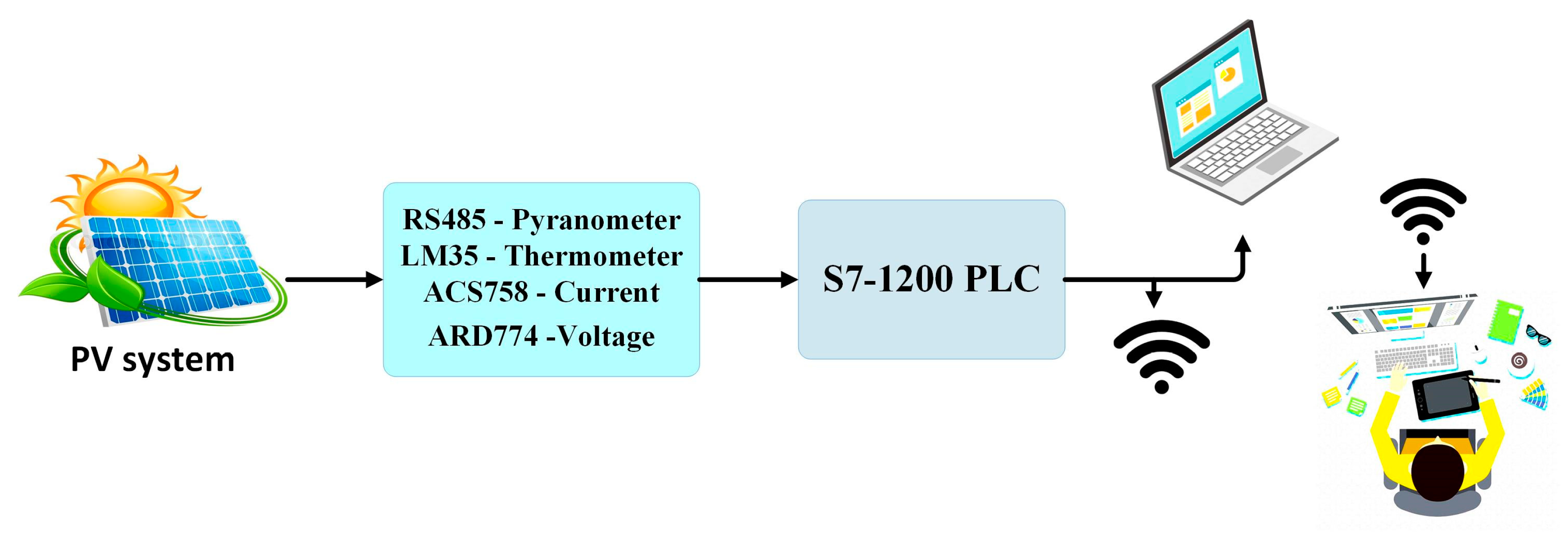
This study utilizes real data obtained from the PV power system situated within the College of Engineering building at the University of Misan, Iraq. The PV data were taken randomly based on six days for each condition state from different seasons of 2024. They were collected at three-minute intervals, spanning from 6 a.m. to 5 p.m. PV generation is influenced by several external elements, including sun radiation, ambient temperature, and cloud cover. Ultimately, the Matplotlib and Seaborn libraries in the Python approach library were utilized to create the visual depictions of the outcomes.

6.1. Sunny Days

The objective of this categorization test is to address the validation of the PV forecasting model in sunny weather circumstances. Precisely, a total of 1158 samples were recorded from 6 days that had clear skies. These samples were uniformly spread among various seasons to depict sunny weather circumstances. In total, 361 samples were taken on the 17th and 22nd of January to represent the winter season. Then, the 12th and 21st of March were chosen to represent the spring season, with a total of 384 samples, while the 7th and 8th of June were selected to represent the summer season, with 413 samples. The number of samples fluctuated due to the incidence of sunlight on the solar panels.

Figure 9 depicts the MAE values, comparing the predicted and actual power generation. The X-axis shows time divided into intervals of 3 min, while the Y-axis represents the MAE in watts. Figure 9a demonstrates that the MAE function of the ANN-GA forecasting model is occasionally the lowest compared to the ANN and ANN-GWO models, as indicated in

Table 3. Summarized prediction results of sunny days for PV model.

Days	Method	RMSE (Watts)	MSE (Watts)	MAE (Watts)	R2
Sunny	ANN	21.5097	462.6680	17.3919	0.9532
	ANN-GA	20.5089	420.6154	16.0403	0.9574
	ANN-GWO	21.8529	477.5520	17.0240	0.9516

. On days with clear skies, the MAE values recorded by the ANN-GA, ANN, and ANN-GWO are 16.0403 W, 17.3919 W, and 17.0240 W, respectively. Meanwhile, the MSE associated with ANN-GA is generally the lowest compared to the ANN and ANN-GWO, as indicated in Figure 10a and Table 3, which refers to the difference between the predicted and actual power generation of the PV system reducing to about 420.6154 W, 462.6080 W, and 477.552 W, respectively. According to the previous values, it is clear that the conventional ANN has a good MAE in sunny weather circumstances compared to the ANN-GWO model. However, it has failed to reach the required values of MSE and RMSE; as periods shift, certain patterns may emerge that impact the performance of each model in distinct ways. Nevertheless, it has been verified that the ANN-GWO model outperforms the ANN model in various conditions characterized by cloudiness and rainfall.

Figure 11a illustrates a comparison test between the theoretical PV power and the actual PV power for the three models during the periods of sunny days. It can be notable that there are fluctuations in the real capacity at various time intervals, with a peak occurring on January 17th at 12:03 p.m. and a trough on 3rd March at 8:25 a.m. Generally, the models are enhanced through the utilization of the GA and the GWO algorithm to exhibit a superior performance and accuracy, as they closely track the actual power levels in both high and low scenarios. In contrast, the basic ANN model drifts away from the standard generation of the PV test. Therefore, employing the optimization methods, such as the GA and GWO algorithm in the NN model, is essentially to enhance the precision of predictions in related applications for energy management and stability of the utilized power grid when it is connected with a PV plant.

6.2. Cloudy Days

In this categorization test, the PV prediction model is proposed for cloudy weather circumstances regarding various seasons. A total of 1063 samples were collected from six evenly distributed cloudy days across various seasons. Specifically, 330 samples were taken on the 2nd and 18th of January to represent the winter season, 356 samples were taken on 11th and 14th of March to represent the spring season, and 377 samples were taken on 22nd and 24th of June to represent the summer season. In overcast weather, the total number of samples is lower compared to bright weather due to the obstruction of sunlight by clouds, which prevents the solar panels from receiving sufficient light. Additionally, the sensor employed may not be sensitive enough to accurately measure the amount of radiation reaching it, resulting in some readings not being recorded.

The findings presented in Figure 9b and Figure 10b indicate the decline in MAE and MSE values for the suggested ANN-GA model. However, it is worth noting that ANN-GA initially exhibited the biggest percentage error during the 18th of January. Nevertheless, the model’s performance improves, subsequently surpassing both ANN and ANN-GWO. Hence, the MAE values range from 0 to 80 W throughout time is determined by computing the mean value of the ANN-GA, ANN, and ANN-GWO models, which are 17.8099 W, 21.8080 W, and 18.1780 W, respectively. Meanwhile, the MSE values for the models are 615.0131 W, 774.8360 W, and 629.6826 W, respectively.

Figure 11b introduces a rapprochement case between the anticipated and actual power generation using the ANN, ANN-GA, and ANN-GWO models in a short term with cloudy weather. Regarding reduction in solar radiation during cloudy weather tests, the production of PV electrical energy decreases throughout these time intervals. Significant spikes in the power consumption can be detected at specific intervals, for instance the day of 1/18 at 4:19 p.m. and during the specific period of day 3/14 at 8:36 a.m. These times occur as a consequence of reduced activity caused by cloud cover obstructing the sun’s radiation. Therefore, it may be inferred that the stable power predictions closely align with the actual capacity of the PV system. Hence, the three models demonstrate accurate prediction during calm periods but, during quick fluctuations, the ANN-GA and ANN-GWO algorithms exhibit superior performance with higher accuracy and more adaptability to the changes in weather conditions. Hence, the R² values for the GA-ANN, ANN, and ANN-GWO are 0.9347, 0.9209, and 0.9332, respectively, as indicated in

Table 4. Summarized prediction results in cloudy days for PV model.

Days	Method	RMSE (Watts)	MSE (Watts)	MAE (Watts)	R2
Cloudy	ANN	27.2917	744.8360	21.8080	0.9209
	ANN-GA	24.7995	615.0131	17.8099	0.9347
	ANN-GWO	25.0934	629.6826	18.1780	0.9332

.

6.3. Rainy Days

In this case, rainy weather circumstances are utilized to assess the proposed PV forecasting prediction model. A total of 809 samples of a rainy state were collected over 6 days distributed across various seasons. To represent the winter season, the heaviest rain days were chosen, which were 11th and 30th of January, to collect 212 samples of these days. Moreover, there were 210 samples on the 19th and 24th of March that represent the spring season and 387 samples on the 20th and 10th of June that represent the summer season. Notably, during January, the duration of daylight hours is decreased in the heavy rainy weather states, which was not recorded in the PV data due to rain-laden clouds blocking radiation. Meanwhile, In June, there was a light rainfall on the 10th owing to the rising temperature. Additionally, a cloudy day was included to make up for the shortage of days with both sunny and cloudy weather. This is because June typically experiences intense sunlight and high temperatures in southern Iraq.

Figure 9c illustrates the MAE observed between forecasted and actual power generation during rainy weather conditions. Based on the data in this figure, it can be shown that the MAE associated with the ANN-GA is occasionally lower than that of both ANN and ANN-GWO, as indicated in

Table 5. Summarized prediction results of rainy days for PV model.

Days	Method	RMSE (Watts)	MSE (Watts)	MAE (Watts)	R2
Rainy	ANN	29.0796	845.6225	16.4599	0.8250
	ANN-GA	22.3597	499.9573	14.3067	0.8965
	ANN-GWO	25.4140	645.8738	15.8127	0.8663

, specifically on the rainfall days. As a result, the MAE values of the suggested models for three proposals were recorded as 14.3067 W, 16.4599 W, and 15.8127 W, respectively.

Figure 10c shows the discrepancy in MSE between predicted and observed power generation during rainy weather conditions that are closer to zero. On one side, the MSE value of the ANN-GWO reaches 30,000 watts during the period from 8 a.m. to 12 noon on 11 January, as well as during the period of 10 to 11 a.m. on 10 June. There is an increase up to 50,000 in the ANN power prediction due to the excessive energy used during these periods, where the peak solar radiation level was recorded at 467.5926 W/m² on 10 June at 10:32 a.m. On the other side, the solar irradiance level was recorded as 193.8658 W/m² and 133.9699 W/m², between this point, in 3 min intervals. In this case, the fluctuation in the ANN prediction happens due to this rapid change in the solar irradiance. This sudden fluctuation in the input irradiance indicates a limitation in its ability to handle rapid variations in the input data of ANN model.

In general, it is noticed that the GA-ANN prediction is the lowest compared to the ANN and ANN-GWO models, as explained in Table 5. Notably, the GA optimization shows consistently the superior performance across different scenarios when the MSE values of the proposed model, ANN, and ANN-GWO are 499.9573 W, 845.6225 W, and 645.8738 W, respectively. Furthermore, Table 5 displays the R² of the proposed model, NN, and NN-GWO, which are reported as 0.8965, 0.8250, and 0.8663, respectively, as shown in Figure 12b, due to a slightly lower correlation compared to clear-sky conditions.

Figure 11 displays the temporal variations in electrical power among the three models during the three-period tests. Figure 11a shows that the values between the real PV power and estimative PV power match roughly when the irradiances are clear on sunny days. Meanwhile, Figure 11b shows less matching between the two power tests on a cloudy day. However, Figure 11c addresses the significant spikes in power levels, namely on 6/10 at 10:18 a.m. This is because of the higher fluctuation recordings for the input irradiance during this time of year when the rain was very heavy and fast, leading to cloud cover blocking the sun’s rays at intervals. Hence, the graph shows sharp fluctuations in power generation on those days. Furthermore, the output energy was diminished compared to sunny and cloudy days due to the presence of rain and clouds, which might obstruct the irradiance reaching the PV panels. This reduction can lead to lower solar energy productivity during rainy days. Nevertheless, the projected values produced by the suggested model continue to closely align with the real energy measurements.

In Figure 12, comparisons of MAE and R² performance measurements across different meteorological seasons are presented. It is provided that the GA-ANN forecasting algorithm accommodates the most accurate PV generation pattern in three different climatic condition tests when compared with the outperformed ANN and ANN-GWO models, as it achieved the highest values of R² under sunny, cloudy, and rainy conditions at about 0.9516, 0.95332, and 0.8663, respectively, when it approached 1 as the degree to which the statistical model successfully predicts the outcome. Meanwhile, it is shown that the MAE values are closer to zero to refer to better prediction performance during the sunny, cloudy, and rainy days at about 17.0240 W, 18.1780 W, and 15.8127 W, respectively.

Figure 13 shows the relative error value between the power prediction and the power generation for the three-day cases. As noticed from Figure 13a, the ANN-GA forecasting model demonstrates the greatest stability compared with the ANN-GWO and the ANN prediction models. In addition, the ANN approach exhibits larger and more pronounced swings, particularly during the periods of days 1/22 and 6/8, where the relative error exceeds 100% and falls below −100%. Hence, the ANN-GA forecasting model achieves the lowest relative percentage error of about 4.5%, while the ANN-GWO and ANN prediction models reach 5.5% and 6%, respectively. Figure 13b exhibits several abrupt changes characterized by significant increases and decreases in the relative inaccuracy when the actual PV power and the predicted PV power of cloudy days are compared. It is noticed that some error rates exceed 400%, while others fall below −100%, indicating the presence of significant flaws in prediction. Hence, it can be provided that the ANN-GA approaches exhibit the highest accuracy and stability in the PV predicting generation as compared to the ANN-GWO and ANN methods. Consequently, the ANN-GA forecasting model acquires the lowest relative percentage error of about 6.5%, while the ANN-GWO and ANN prediction models reach 7% and 12.5%, respectively.

Finally, Figure 13c illustrates a consistently constant relative error around zero for long periods in rainy weather. However, there is a specific period, namely 3/24 at 9:24 a.m., during which significant and abrupt negative fluctuations occur. These fluctuations result in a substantial decrease in relative error, reaching values as low as −5000% for all methods. This is because the PV system is influenced by fluctuations in weather conditions, as its performance is closely tied to the level of solar radiation that is significantly low and varies on rainy days. As a results, the ANN-GA forecasting model acquires the lowest relative percentage error of about 40%, while the ANN and ANN-GWO prediction models reach 44% and 56.5%, respectively.

Lastly,

Table 6. Relative percentage error for sunny, cloudy, and rainy days.

Method	Sunny Days	Cloudy Days	Rainy Days
ANN-GA	4.5%	6.5%	40%
ANN-GWO	5.5%	7%	56.5%
ANN	6%	12.5%	44%

summarizes the comparison of PV energy regarding relative percentage errors for three categorization tests. It is demonstrated that enhancing PV prediction is a crucial objective to increase the unpredictability of weather conditions on rainy and overcast days. As a result, the ANN has been developed by using two different algorithms. Hence, the ANN-GA prediction model outperforms the other approaches in all-weather circumstances, since the measured values of the fitness functions were significantly lower than those of the other methods, indicating the commendable performance of this model. On the other hand, the main limitation of this research is that the PV data have been used as specific to a particular region, and only temperature and solar radiation were considered as inputs for the proposed models. It will be better to collect the PV data from various regions, with potential improvements by incorporating additional inputs such as humidity, dust, and other meteorological factors that could influence the accuracy of PV prediction.

Finally, the previous studies that have been mentioned in this paper focused on designing the PV power prediction models based on different techniques. Meanwhile, our research used very recent data collected from the year of 2024, which set it apart from previous works. In addition, two different NN optimization methods were implemented to compare between them. The results showed almost similar performance when compared to the research conducted by researchers in [46], which used a 5 min time resolution. The study reported an RMSE of 19.87%, while our research yielded an RMSE of 20.5089 for sunny weather conditions, despite the differences in the proposed methodologies. Furthermore, the study that was conducted by researchers in [47], North China, which focused on the winter period from 2016 to 2018, showed an RMSE of 6.23 MWh for clear days. In comparison, we found an RMSE of 20.5089 watts for clear days that indicates the accuracy and effectiveness of the proposed methods, even when considering different weather conditions and data ranges.

7. Conclusions

This study has designed a PV forecasting model based on machine learning approaches to assess the effective production of PV power in the geographic areas of Iraq for the first time. To summarize, real data of the PV system installed at the University of Misan/college of Engineering are collected at intervals every three minutes of daily production to analyze the PV effectiveness based on the ANN model. This model combines two different advanced optimization algorithms, GA and GWO techniques, to regulate the elements of the ANN model. Rainy, cloudy, and sunny days for different seasons are tested to address the performance of the forecasting models under various weather conditions. Finally, they have been evaluated based on four statistical measures: R², MAE, RMSE, and MSE. The methodology of training the ANN model using the GA optimization has shown that it is efficient to determine the ideal number of layers and neurons of the ANN model, resulting in adjusting the lower fitness functions. Consequently, the relative percentage error value between the PV prediction and the PV generation is the lowest at about 4.5%, 6.5%, and 40% for sunny, cloudy, and rainy days, respectively. In addition, the findings showed that the MAE value of the ANN-GA model was 14.3067, 17.8099, and 16.0403 watts for rainy, cloudy, and sunny weather, respectively. Hence, the GA-NN forecasting model has achieved remarkable precision, more reliability, and excellent performance in predicting the actual PV power under various weather conditions. It is imperative in future research to explore more suitable methodologies in different scenarios to enhance the accuracy of PV predictions.

References

1. Ting, D.S.-K. Green Illusions: The Dirty Secrets of Clean Energy and the Future of Environmentalism. Int. J. Environ. Stud. 2013, 70, 832–835. [Google Scholar] [CrossRef]
2. System, P.; Adaptive, U.; Dawan, P.; Sriprapha, K.; Kittisontirak, S.; Boonraksa, T. Comparison of Power Output Forecasting on the Inference Systems and Particle Swarm. Energies 2020, 13, 351. [Google Scholar] [CrossRef]
3. Colak, M.; Yesilbudak, M.; Bayindir, R. Daily Photovoltaic Power Prediction Enhanced by Hybrid GWO-MLP, ALO-MLP and WOA-MLP Models Using Meteorological Information. Energies 2020, 13, 901. [Google Scholar] [CrossRef]
4. Al-Messabi, N.; Li, Y.; El-Amin, I.; Goh, C. Forecasting of Photovoltaic Power Yield Using Dynamic Neural Networks. In Proceedings of the 2012 International Joint Conference on Neural Networks (IJCNN), Brisbane, QLD, Australia, 10–15 June 2012; IEEE: New York, NY, USA, 2012; pp. 1–5. [Google Scholar] [CrossRef]
5. Almonacid, F.; Pérez-Higueras, P.J.; Fernández, E.F.; Hontoria, L. A Methodology Based on Dynamic Artificial Neural Network for Short-Term Forecasting of the Power Output of a PV Generator. Energy Convers. Manag. 2014, 85, 389–398. [Google Scholar] [CrossRef]
6. Antonanzas, J.; Osorio, N.; Escobar, R.; Urraca, R.; Martinez-de-Pison, F.J.; Antonanzas-Torres, F. Review of Photovoltaic Power Forecasting. Sol. Energy 2016, 136, 78–111. [Google Scholar] [CrossRef]
7. Hussein, A.R.; Dakhil, A.M.; Rashed, J.R.; Othman, M.F. Intelligent Expert System for Diagnosing Faults and Assessing Quality of Power Transformer Insulation Oil by DGA Method. Misan J. Eng. Sci. 2022, 1, 47–57. [Google Scholar] [CrossRef]
8. Panapakidis, I.P.; Christoforidis, G.C. A Hybrid ANN/GA/ANFIS Model for Very Short-Term PV Power Forecasting. In Proceedings of the 2017 11th IEEE International Conference on Compatibility, Power Electronics and Power Engineering (CPE-POWERENG), Cadiz, Spain, 4–6 April 2017; IEEE: New York, NY, USA, 2017; pp. 412–417. [Google Scholar] [CrossRef]
9. Semero, Y.K.; Zhang, J.; Zheng, D. PV Power Forecasting Using an Integrated GA-PSO-ANFIS Approach and Gaussian Process Regression Based Feature Selection Strategy. CSEE J. Power Energy Syst. 2018, 4, 210–218. [Google Scholar] [CrossRef]
10. Semero, Y.K.; Zheng, D.; Zhang, J. A PSO-ANFIS Based Hybrid Approach for Short Term PV Power Prediction in Microgrids. Electr. Power Compon. Syst. 2018, 46, 95–103. [Google Scholar] [CrossRef]
11. AlShafeey, M.; Csáki, C. Evaluating Neural Network and Linear Regression Photovoltaic Power Forecasting Models Based on Different Input Methods. Energy Rep. 2021, 7, 7601–7614. [Google Scholar] [CrossRef]
12. Adeyemi, K.O.; Eniola, V.; Kalu-Uka, G.M.; Zarmai, M.; Uthman, M.; Bala, E. Forecasting Photovoltaic Energy Generation Using Multilayer Perceptron Neural Network. Int. J. Renew. Energy Res. 2022, 12, 1742–1753. [Google Scholar] [CrossRef]
13. Netsanet, S.; Zheng, D.; Zhang, W.; Teshager, G. Short-Term PV Power Forecasting Using Variational Mode Decomposition Integrated with Ant Colony Optimization and Neural Network. Energy Rep. 2022, 8, 2022–2035. [Google Scholar] [CrossRef]
14. Alrashidi, M.; Rahman, S. Short-Term Photovoltaic Power Production Forecasting Based on Novel Hybrid Data-Driven Models. J. Big Data 2023, 10, 26. [Google Scholar] [CrossRef]
15. Li, G.; Xie, S.; Wang, B.; Xin, J.; Li, Y.; Du, S. Photovoltaic Power Forecasting with a Hybrid Deep Learning Approach. IEEE Access 2020, 8, 175871–175880. [Google Scholar] [CrossRef]
16. Bendali, W.; Saber, I.; Bourachdi, B.; Boussetta, M.; Mourad, Y. Deep Learning Using Genetic Algorithm Optimization for Short Term Solar Irradiance Forecasting. In Proceedings of the 2020 Fourth International Conference on Intelligent Computing in Data Sciences (ICDS), Fez, Morocco, 21–23 October 2020; IEEE: New York, NY, USA, 2020; pp. 1–8. [Google Scholar] [CrossRef]
17. Aprillia, H.; Yang, H.T.; Huang, C.M. Short-Term Photovoltaic Power Forecasting Using a Convolutional Neural Network-Salp Swarm Algorithm. Energies 2020, 13, 1879. [Google Scholar] [CrossRef]
18. Li, S.; Li, R.; Yang, J.; Wu, F.; Rashed, G.I. Combined Prediction of Photovoltaic Power Based on Sparrow Search Algorithm Optimized Convolution Long and Short-Term Memory Hybrid Neural Network. Electronics 2022, 11, 1654. [Google Scholar] [CrossRef]
19. Li, L.L.; Zhao, X.; Tseng, M.L.; Tan, R.R. Short-Term Wind Power Forecasting Based on Support Vector Machine with Improved Dragonfly Algorithm. J. Clean. Prod. 2020, 242, 118447. [Google Scholar] [CrossRef]
20. Pan, M.; Li, C.; Gao, R.; Huang, Y.; You, H.; Gu, T.; Qin, F. Photovoltaic Power Forecasting Based on a Support Vector Machine with Improved Ant Colony Optimization. J. Clean. Prod. 2020, 277, 123948. [Google Scholar] [CrossRef]
21. Liu, Y.W.; Feng, H.; Li, H.Y.; Li, L.L. An Improved Whale Algorithm for Support Vector Machine Prediction of Photovoltaic Power Generation. Symmetry 2021, 13, 212. [Google Scholar] [CrossRef]
22. Gueymard, C.A. The Sun’s Total and Spectral Irradiance for Solar Energy Applications and Solar Radiation Models. Sol. Energy 2004, 76, 423–453. [Google Scholar] [CrossRef]
23. Gordillo, G. Photoluminescence and Photoconductivity Studies on ZnxCd1-XS Thin Films. Sol. Energy Mater. Sol. Cells 1992, 25, 41–49. [Google Scholar] [CrossRef]
24. Jacobson, M.Z.; Delucchi, M.A. Providing All Global Energy with Wind, Water, and Solar Power, Part I: Technologies, Energy Resources, Quantities and Areas of Infrastructure, and Materials. Energy Policy 2011, 39, 1154–1169. [Google Scholar] [CrossRef]
25. Das, U.K.; Tey, K.S.; Seyedmahmoudian, M.; Mekhilef, S.; Idris, M.Y.I.; Van Deventer, W.; Horan, B.; Stojcevski, A. Forecasting of Photovoltaic Power Generation and Model Optimization: A Review. Renew. Sustain. Energy Rev. 2018, 81, 912–928. [Google Scholar] [CrossRef]
26. Al-Majidi, S.D.; Abbod, M.F.; Al-Raweshidy, H.S. A Particle Swarm Optimisation-Trained Feedforward Neural Network for Predicting the Maximum Power Point of a Photovoltaic Array. Eng. Appl. Artif. Intell. 2020, 92, 103688. [Google Scholar] [CrossRef]
27. Kaplanis, S.; Kaplani, E.; Kaldellis, J.K. PV Temperature Prediction Incorporating the Effect of Humidity and Cooling Due to Seawater Flow and Evaporation on Modules Simulating Floating PV Conditions. Energies 2023, 16, 4756. [Google Scholar] [CrossRef]
28. Sedai, A.; Dhakal, R.; Gautam, S.; Dhamala, A.; Bilbao, A.; Wang, Q.; Wigington, A.; Pol, S. Performance Analysis of Statistical, Machine Learning and Deep Learning Models in Long-Term Forecasting of Solar Power Production. Forecasting 2023, 5, 256–284. [Google Scholar] [CrossRef]
29. Roumpakias, E.; Stamatelos, T. Prediction of a Grid-Connected Photovoltaic Park’s Output with Artificial Neural Networks Trained by Actual Performance Data. Appl. Sci. 2022, 12, 6458. [Google Scholar] [CrossRef]
30. Mojumder, J.C.; Ong, H.C.; Chong, W.T.; Izadyar, N.; Shamshirband, S. The Intelligent Forecasting of the Performances in PV/T Collectors Based on Soft Computing Method. Renew. Renew. Sustain. Energy Rev. 2017, 72, 1366–1378. [Google Scholar] [CrossRef]
31. Zhang, C.; Zhang, M. Wavelet-Based Neural Network with Genetic Algorithm Optimization for Generation Prediction of PV Plants. Energy Rep. 2022, 8, 10976–10990. [Google Scholar] [CrossRef]
32. Akhter, M.N.; Mekhilef, S.; Mokhlis, H.; Shah, N.M. Review on Forecasting of Photovoltaic Power Generation Based on Machine Learning and Metaheuristic Techniques. IET Renew. Power Gener. 2019, 13, 1009–1023. [Google Scholar] [CrossRef]
33. Pang, Z.; Niu, F.; O’Neill, Z. Solar Radiation Prediction Using Recurrent Neural Network and Artificial Neural Network: A Case Study with Comparisons. Renew. Energy 2020, 156, 279–289. [Google Scholar] [CrossRef]
34. Singla, P.; Duhan, M.; Saroha, S. A Comprehensive Review and Analysis of Solar Forecasting Techniques. Front. Energy 2021, 16, 187–223. [Google Scholar] [CrossRef]
35. Al-majidi, S.D.; Dawood, H.; Altai, S.; Lazim, M.H.; Al-nussairi, M.K.; Abbod, M.F.; Al-raweshidy, H.S. Bacterial Foraging Algorithm for a Neural Network Learning Improvement in an Automatic Generation Controller. Energies 2023, 16, 2802. [Google Scholar] [CrossRef]
36. Radhi, S.M.; Al-majidi, S.D.; Abbod, M.F.; Al-raweshidy, H.S. Predicting Solar Power Generation Utilized in Iraq Power Grid Using Neural Network. Misan J. Eng. Sci. 2024, 3, 38–62. [Google Scholar] [CrossRef]
37. Wu, Z.; Wang, B. An Ensemble Neural Network Based on Variational Mode Decomposition and an Improved Sparrow Search Algorithm for Wind and Solar Power Forecasting. IEEE Access 2021, 9, 166709–166719. [Google Scholar] [CrossRef]
38. Dawood, H.; Altai, S.; Lpizra, A.; Saleh, A.L.; Tuama, H.; Lazim, M.H. Solving Unit Commitment Including Wind Power Generation Using PSS® E. Misan J. Eng. Sci. 2022, 1, 69–93. [Google Scholar] [CrossRef]
39. Saadaoui, D.; Elyaqouti, M.; Assalaou, K.; Ben Hmamou, D.; Lidaighbi, S. Parameters Optimization of Solar PV Cell/Module Using Genetic Algorithm Based on Non-Uniform Mutation. Energy Convers. Manag. X 2021, 12, 100129. [Google Scholar] [CrossRef]
40. Sivanandam, S.N.; Deepa, S.N. Introduction to Genetic Algorithms; Springer: Berlin/Heidelberg, Germany, 2008; pp. 1–442. ISBN 9783540731894. [Google Scholar] [CrossRef]
41. Hassanat, A.B.; Prasath, V.B.S.; Abbadi, M.A.; Abu-Qdari, S.A.; Faris, H. An Improved Genetic Algorithm with a New Initialization Mechanism Based on Regression Techniques. Information 2018, 9, 167. [Google Scholar] [CrossRef]
42. Gupta, D.; Ghafir, S. An Overview of Methods Maintaining Diversity in Genetic Algorithms. Int. J. Emerg. Technol. Adv. Eng. 2012, 2, 56–60. [Google Scholar]
43. Mirjalili, S.; Mirjalili, S.M.; Lewis, A. Grey Wolf Optimizer. Adv. Eng. Softw. 2014, 69, 46–61. [Google Scholar] [CrossRef]
44. Mosavi, S.K.; Jalalian, E.; Gharahchopog, F.S. A Comprehensive Survey of Grey Wolf Optimizer Algorithm and Its Application. Int. J. Adv. Robot. Expert Syst. (JARES) 2018, 1, 23–45. [Google Scholar]
45. Lawah, A.I.; Ibrahim, A.A.; Salih, S.Q.; Alhadawi, H.S.; Josephng, P.S. Grey Wolf Optimizer and Discrete Chaotic Map for Substitution Boxes Design and Optimization. IEEE Access 2023, 11, 42416–42430. [Google Scholar] [CrossRef]
46. Pan, X.; Zhou, J.; Sun, X.; Cao, Y.; Cheng, X.; Farahmand, H. A Hybrid Method for Day-Ahead Photovoltaic Power Forecasting Based on Generative Adversarial Network Combined with Convolutional Autoencoder. IET Renew. Power Gener. 2023, 17, 644–658. [Google Scholar] [CrossRef]
47. Meng, M.; Song, C. Daily Photovoltaic Power Generation Forecasting Model Based on Random Forest Algorithm for North China in Winter. Sustainability 2020, 12, 2247. [Google Scholar] [CrossRef]
Figure 1. The classification of PV power prediction.
Energies 17 04301 g001
Figure 2. The block diagram of a neural network.
Energies 17 04301 g002
Figure 3. Graphical processing of a GWO algorithm.
Energies 17 04301 g003
Figure 4. The system architecture of a data acquisitor system.
Energies 17 04301 g004
Figure 5. The outdoor PV system combined at the Engineering campus of University Misan, Iraq.
Energies 17 04301 g005
Figure 6. The framework of ANN-GA for PV power forecasting.
Energies 17 04301 g006
Figure 7. The framework of ANN-GWO for PV power forecasting.
Energies 17 04301 g007
Figure 8. The methodology of training stages.
Energies 17 04301 g008
Figure 9. The result of MAE based on ANN, ANN-GA, and ANN-GWO for (a) sunny days, (b) cloudy days, and (c) rainy days.
Energies 17 04301 g009
Figure 10. The result of MSE based on ANN, ANN-GA, and ANN-GWO for (a) sunny days, (b) cloudy days, and (c) rainy days.
Energies 17 04301 g010
Figure 11. The relationship between actual power and prediction power based on ANN, ANN-GA, and ANN-GWO for (a) sunny days, (b) cloudy days, and (c) rainy days.
Energies 17 04301 g011
Figure 12. Comparison of MAE and R2 performance measurements across different meteorological seasons. (a) Sunny days, (b) cloudy days, and (c) rainy days.
Energies 17 04301 g012aEnergies 17 04301 g012b
Figure 13. Relative error (%) with ANN, ANN-GA, and ANN-GWO on (a) sunny days, (b) cloudy days, and (c) rainy days.
Energies 17 04301 g013