Whale Optimization Algorithm BP Neural Network with Chaotic Mapping Improving for SOC Estimation of LMFP Battery

Abstract

The state of charge (SOC) is a core parameter in the battery management system for LMFP batteries. Accurate SOC estimation is crucial for ensuring the safety and reliability of energy storage applications and new energy vehicles. In order to achieve better SOC estimation accuracy, this article proposes an adaptive whale optimization algorithm (WOA) with chaotic mapping to improve the BP neural network (BPNN) model. The SOC estimation accuracy of the BPNN model was improved by utilizing WOA to find the optimal target weight values and thresholds. Comparative simulation experiments (including constant current and working condition discharge experiments) were conducted in Matlab/Simulink R2018a to verify the proposed algorithm and the other four algorithms. The experimental results show that the proposed algorithm had higher SOC estimation accuracy than the other four algorithms, and its prediction errors were less than 1%. This indicates that the proposed SOC estimation method has better prediction accuracy and stability, and has certain theoretical research significance.

1. Introduction

The rapid development of industry has brought prosperity to the economy. At the same time, the global energy crisis and environmental pollution problems have also accelerated. As a substitute for traditional fuel, novel energy storage solutions and new energy vehicles have attracted attention from both industry and academia in recent years. LMFP batteries have become the preferred power source for energy storage and new energy vehicles due to their high energy density, long cycle life, low self-discharge rate, and lack of memory effect [1,2]. As an upgrade of LFP, LMFP theoretically improves battery energy density by 15–20%, and its safety performance is better than that of NCM/NCA Li-ion batteries. In addition, LMFP batteries have a low dependence on rare metals and pose a significant cost advantage. The SOC of the LMFP battery is used to measure the power stored in the current battery, and a key parameter in the battery management system of energy storage and new energy vehicles. Accurate battery SOC estimation can avoid over-charge or over-discharge of the battery, extend the service life of the battery, and improve the use safety of the battery system [3,4]. However, due to the complex electrochemical nature of LMFP batteries, the SOC cannot be directly measured, and can only be estimated.

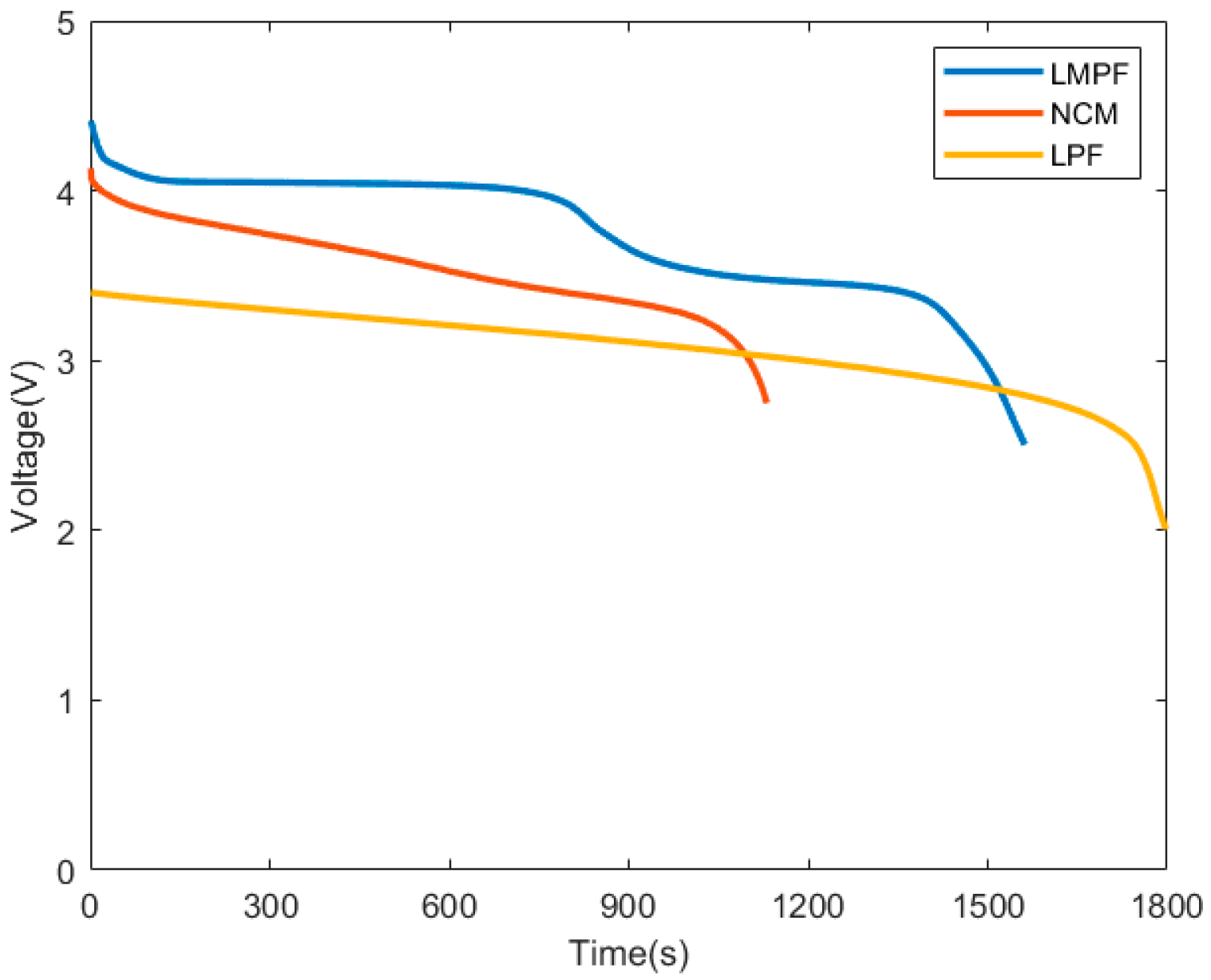
The LMFP battery has become a research hotspot for olivine type cathode materials due to its significant advantages of high specific energy, high safety, and low cost. From the perspective of energy density, LMFP battery material has the characteristic of dual voltage platforms. It can be seen from Figure 1 that when comparing LMFP, LFP, and NCM batteries, there is a significant decrease in the voltage plateau of the LMFP battery in the middle of the discharge process, which makes it hard to estimate the SOC.

At present, there are four methods that are usually used for estimating the SOC of Li-ion batteries. These include direct measurement, the model-driven method, the data- driven method, and the combination-optimization method.

(i)

Direct measurement: methods for direct measurement include ampere hour integration, open circuit voltage, and discharge testing. Ampere hour integration estimates battery SOC based on the integration of the current value flowing through the battery and time. This method is simple and reliable. However, it requires high measurement accuracy for the initial SOC measurement value of the battery and the measurement value of the battery current, and is prone to accumulated errors during the continuous integration of the estimation process [5]. Open circuit voltage estimates SOC by searching for the corresponding functional relationship between the open circuit voltage of a battery and the SOC. This method is simple and easy to implement, but it requires long rest periods for the battery to obtain the open circuit voltage. It is also limited by working environment conditions and is not suitable for online real-time calculation [6,7]. The discharge test calculates the battery SOC by multiplying the constant discharge current and discharge time. This method has the advantages of simplicity and reliability, but it cannot meet the requirements of online SOC estimation due to its long measurement time [8].

(ii)

Model-driven method: these methods need to first establish a battery model, such as an electrochemical model, equivalent circuit model, etc. Then, the battery model is combined with adaptive filtering algorithms (such as the Kalman filter algorithm, extended Kalman filter (EKF) algorithm, particle filter algorithm, etc.) to estimate the battery SOC [9,10,11]. This method can achieve online measurement and has good self-correction ability and adaptability, but it is often difficult and time-consuming to establish a detailed and well described battery model representing the external characteristics of the battery. Moreover, the performance of these methods is limited by inaccurate battery models, and the computational complexity of identifying the dynamic external parameters of the battery model also limits their online application [12,13].

(iii)

Data-driven method: these methods usually need to learn and train a large number of sample data of battery-related measurable variables to find the nonlinear mapping relationship between them and battery SOC [14,15]. The most frequently used methods include artificial neural networks (ANN) [16,17,18,19], support vector machines (SVM) [20], RNN, LSTM [21,22,23,24], GRU [25], fuzzy logic, Gaussian process regression, etc. These are extensively used as they accurately map nonlinearity, enabling short-term forecasting. Salkind et al. [26] applied fuzzy logic to estimate the SOC and SOH of Li-ion batteries. Anton et al. [27] employed a SVM to estimate battery SOC from current, voltage, and temperature. ANNs have been widely used due to their strong nonlinear fitting ability to simulate the complex structure inside batteries. Kang et al. [28] proposed an ANN to estimate the SOC of Li-ion batteries under varying aging levels. The main advantage of information fusion-based models is that they appropriately represent the nonlinear behavior of the battery charging and discharging process due to the training process [29].

(iv)

Combination optimization method: these methods use several advancements and improvements that have made the conventional ANN more effective [30]. In [31], in order to solve easy to fall into the local maximum optimal solution of the traditional NN, a fireworks elite genetic (FEG) algorithm was adopted to improve the BPNN. The effect of the combination algorithm was enhanced, the result error was reduced, and the spread speed was faster. In [32], in order to optimize the weights and thresholds of BPNN, Levy’s flight combined with a particle swarm optimization (PSO) algorithm was proposed, which would make the SOC more accurate. In [33], a BPNN combined with a multi-population genetic algorithm (MPGA) was used to compensate for nonlinear errors and to avoid the immature genetic algorithm (GA) phenomenon. In [34], optimization of the BPNN using the tuna swarm optimization algorithm was adopted to improve the EKF algorithm for accurate SOC estimation. In [35], an improved sparrow search algorithm optimized BPNN was proposed for Li-ion battery SOC estimation in order to improve the accuracy and the global optimal solution. In [36], the PSO algorithm was adopted to improve RBFNN estimation, which improved the accuracy of the estimation results.

Many artificial intelligence and machine learning methods are also widely used. Hang et al. [37]’s extreme learning machine was proposed to address the slow training and local minima convergence of traditional ANNs. In [38], an improved firefly algorithm model combined with Gaussian process regression was used and compared with a conventional method and swarm intelligence algorithms. In [39], a chaotic firefly-particle filtering algorithm was presented, which used chaotic mapping to find a new optimal solution in a group of particles and realize high-precision estimation. In [40], a metaheuristic algorithm, namely, the evolutionary mating algorithm (EMA) was proposed to optimize deep learning (DL) parameters for estimating the battery SOC. In [41], a grey wolf optimization (GWO) algorithm with a fast convergence strategy for the co-estimation of battery capacity and SOC was proposed. The presented algorithm optimized the initial noise covariance of the EKF algorithm by using GWO. In [42,43], an improved extreme learning machine (ELM) based on the SOC estimation model is proposed. Because ELM performance is extremely dependent on network hidden layer biases and weights, a salp swarm algorithm (SSA) was adopted to look for the coefficients, and chaotic mapping was adopted to make the initialized individuals uniformly distributed. In [44], a resistance-capacitance model combined with a Gaussian PSO particle filter was proposed for SOC estimation. It exploited the strong optimality-seeking ability of the PSO, suppressing algorithm degradation and particle impoverishment by improving the importance distribution. In [45], a self-adaptive PSO differential evolution algorithm was proposed, using an optimizing objective function to minimize errors. In [46], the author provides a detailed overview of various types of algorithms currently used for SOC estimation in Li-ion batteries and makes reasonable classifications.

However, data-driven and combination optimization methods still have shortcomings, such as poor robustness and insufficient accuracy. BPNN has disadvantages such as slow learning speed, easy falling into local minima, limited network layers, and over-fitting [47].

In response to the above issues, this article will optimize and improve the standard BPNN through the whale optimization algorithm with chaotic mapping in order to improve the performance (such as slow convergence speed, poor robustness, and being prone to falling into local minima) of the network model and further improve the accuracy of the estimation results.

The remainder of this paper is organized as follows. Section 2 describes the standard BPNN and whale optimization algorithm. Section 3 describes the whale optimization algorithm combined with the BPNN algorithm. Section 4 describes the use of chaotic mapping in improving the whale optimization algorithm. The simulation and experimental results are discussed in Section 5. Finally, the main conclusions of this work are summarized.

2. Standard BPNN and WOA

2.1. Standard BPNN

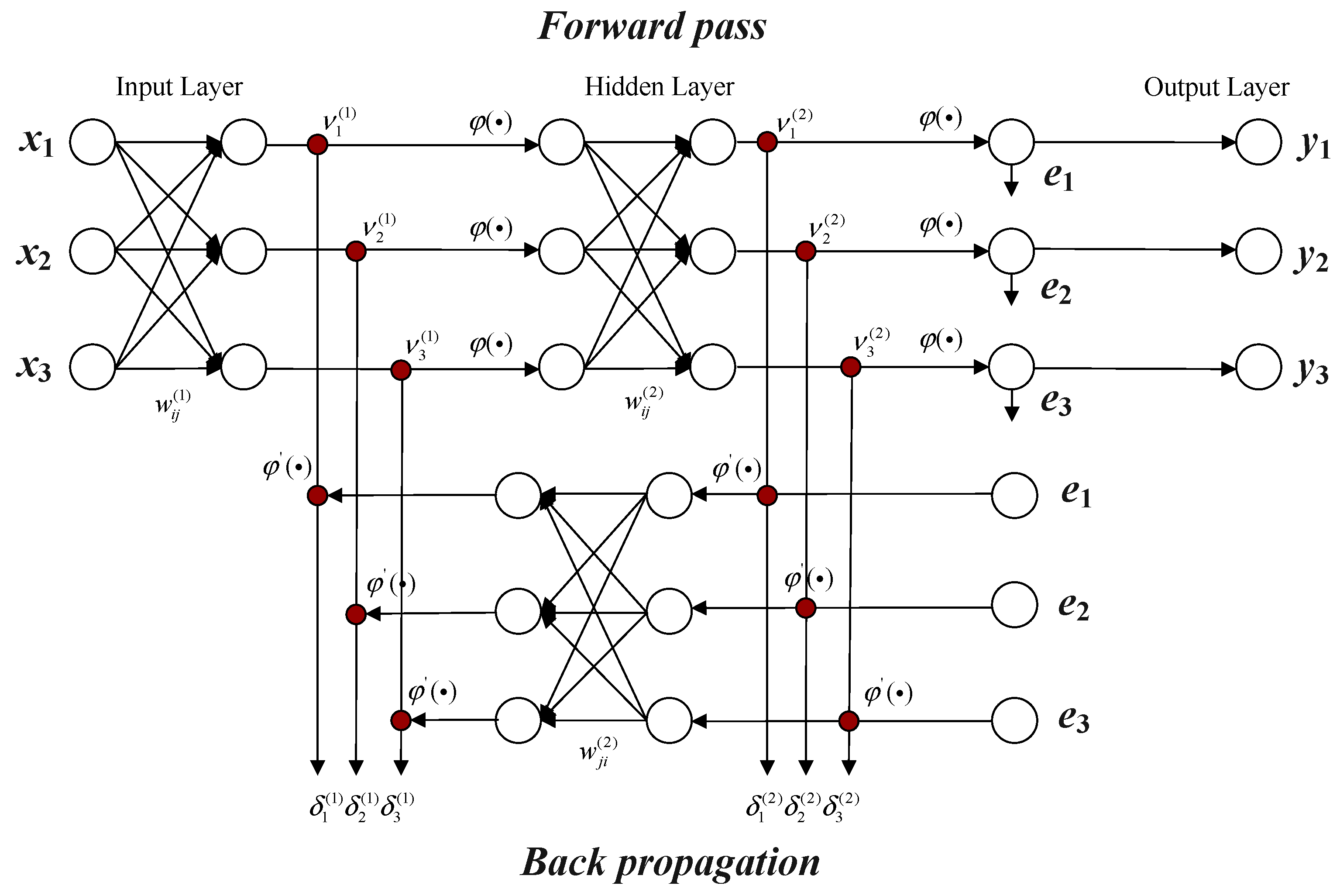
BPNN is a multi-layer feed forward neural network trained according to the error backpropagation algorithm. Its main characteristics are input signal forward propagation and error backpropagation. In forward propagation, input data is fed into the input layer and processed through the hidden layer to obtain the output layer’s results. At this stage, the signal from the input layer is passed to the hidden layer through weighted sum operation. The neurons in the hidden layer receive the signal from the previous layer, process it through the activation function, and then pass it on to the next layer until it finally reaches the output layer. The output of each layer is the source of input for the next layer. If the output layer cannot obtain the expected output, it enters the backpropagation stage. By calculating the error of the output layer, the error is propagated forward layer by layer, and the weight and threshold of each neuron are updated to minimize the error function, so that the predicted output of the BPNN continuously approaches the expected output. The core of the backpropagation stage is the chain rule, which calculates the partial derivatives of errors on weights and thresholds to achieve updates. BPNN can have multiple hidden layers, and an increase in the number of hidden layers can further improve the complexity and expression ability of the model, thereby better adapting to complex data distribution and patterns. In practical applications, while ensuring network and generalization capabilities, the selection of the number of hidden layers should strive to make the entire network structure more compact [48,49].

The topology structure of a standard three-layer BPNN is shown in Figure 2.

2.2. Standard WOA

WOA is an intelligent swarm-based metaheuristic optimization algorithm, inspired by the behavior of humpback whales hunting prey. Figure 3 shows the classical hunting method of humpback whales. The standard WOA simulates the classical hunting method and surrounding or attacking mechanism of humpback whales, including three stages: hunting prey, bubble net hunting, and random hunting of prey. In WOA, the position of each whale represents a potential solution, and the position of the prey captured by the whale is the global optimal solution. Compared with other algorithms, WOA has the advantages of simple structure, fewer parameter settings, and strong search ability.

(i)

Hunting prey

The search scope of the WOA algorithm is the entire solution space, and the algorithm initially assumes that the location of the current prey is the global optimal solution location. Then, the humpback whales in the population will gather towards the prey. When the humpback whales gather towards the prey, their position will change. At this time, the mathematical model of the humpback whale’s position is represented by Equations (1) and (2):

$$\mathrm{D}=\left|\mathrm{C}·{\mathrm{X}}^{\ast }(\mathrm{t})-\mathrm{X}(\mathrm{t})\right|$$

(1)

$$\mathrm{X}(\mathrm{t}+1)={\mathrm{X}}^{\ast }(\mathrm{t})-\mathrm{A}·\mathrm{D}$$

(2)

where D represents the distance between a humpback whale and its prey, ${\mathrm{X}}^{\ast }(\mathrm{t})$ represents the position vector of the current optimal solution, $\mathrm{X}(\mathrm{t})$ represents the current position of the humpback whale, t represents the current number of iterations, and A and C represent coefficient vectors, as seen in Equations (3) and (4):

$$\mathrm{A}=2\mathrm{a}\ast {\mathrm{r}}_1-\mathrm{a}$$

(3)

$$\mathrm{C}=2\ast {\mathrm{r}}_2$$

(4)

where ${\mathrm{r}}_1$ and ${\mathrm{r}}_2$ represents random vectors in intervals $[0,1]$, and a represents a linear convergence factor that linearly decreases from 2 to 0 during the iteration process.

(ii)

Bubble web hunting

Humpback whales mainly hunt through two mechanisms: surrounding prey and executing bubble net attacks. During hunting, humpback whales approach their prey in a spiral upward motion, which in turn feeds on them. The position update between humpback whales and prey is represented by a logarithmic spiral equation, and its mathematical model is shown in Equations (5) and (6):

$$\mathrm{X}(\mathrm{t}+1)={\mathrm{D}}^{\prime }\ast {\mathrm{e}}^{\mathrm{b}\mathrm{l}}\ast \mathrm{c}\mathrm{o}\mathrm{s}(2\mathsf{\pi }\mathrm{l})+{\mathrm{X}}^{\ast }(\mathrm{t})$$

(5)

$${\mathrm{D}}^{\prime }=\left|{\mathrm{X}}^{\ast }(\mathrm{t})-\mathrm{X}(\mathrm{t})\right|$$

(6)

where, D represents the distance between the current humpback whale and its prey, b represents the spiral shape parameters, and l represents a random number in $\left[\mathrm{0,1}\right]$.

There are two hunting behaviors of humpback whales when approaching their prey. Assuming that the probability of each humpback whale randomly choosing two hunting behaviors is 50%, the updated mathematical model of the position of humpback whales can be obtained as Equation (7):

$$\mathrm{X}(\mathrm{t}+1)=\left\{\begin{array}{c}{\mathrm{X}}^{\ast }(\mathrm{t})-\mathrm{A}\ast \mathrm{D} \mathrm{p}\le 0.5\\ {\mathrm{D}}^{\prime }\ast {\mathrm{e}}^{\mathrm{b}\mathrm{l}}\ast \mathrm{c}\mathrm{o}\mathrm{s}(2\mathrm{\pi }\mathrm{l})+{\mathrm{X}}^{\ast }(\mathrm{t}) \mathrm{p}\ge 0.5 \end{array}\right.$$

(7)

where p represents the probability of a hunting mechanism, and p is a random number in $[0,1]$.

(iii)

Random search for prey

As the number of iterations (t) increases, the parameter A in Equation (2) will gradually decrease. When $\left|\mathrm{A}\right|<1$, each humpback whale will gradually surround the current optimal solution; at this point, the algorithm is in the local optimization stage. To ensure that all humpback whales can search adequately in the solution space, the algorithm updates the position based on the distance between each humpback whale in order to achieve the goal of random search. Therefore, when $\left|\mathrm{A}\right|\ge 1$, The current position of a humpback whale will be randomly selected as a reference to update the positions of other humpback whales, allowing the humpback whale population to conduct a global search and avoid being in local optimization. The mathematical model of the position of the humpback whale is obtained using Equations (8) and (9):

$${\mathrm{D}}^{″}=\left|\mathrm{C}\ast {\mathrm{X}}_{\mathrm{r}\mathrm{a}\mathrm{n}\mathrm{d}}(\mathrm{t})-\mathrm{X}(\mathrm{t})\right|$$

(8)

$$\mathrm{X}(\mathrm{t}+1)={\mathrm{X}}_{\mathrm{r}\mathrm{a}\mathrm{n}\mathrm{d}}(\mathrm{t})-\mathrm{A}\ast \mathrm{D}$$

(9)

where ${\mathrm{D}}^{″}$ represents the distance between the currently searched and a random humpback whale, and ${\mathrm{X}}_{\mathrm{r}\mathrm{a}\mathrm{n}\mathrm{d}}(\mathrm{t})$ represents the position of a random humpback whale in the current population.

In [50], WOA is discussed, covering its algorithmic background, possible hybrids, constraints, traits, and application. Deng et al. [51] initialized the population using chaotic mapping to prevent the WOA deviating away from the optimal value. The authors modified the population and combined the pheromones of the black widow algorithm and an adversarial learning strategy to improve the overall performance and convergence speed of WOA. They designed an adaptive coefficient and a new update mode to replace the original mode, making the WOA simpler and more accurate. Yang et al. [52] improved the algorithm by using adaptive strategies and a Lévy flight strategy, achieving a dynamic balance between global exploration and local development, and enhancing the search area of the algorithm. Liu et al. [53] introduced a roulette wheel selection mechanism to address the shortcomings of the original WOA, in order to eliminate inferior solutions and improve convergence speed. It used a dual population interactive evolution strategy with a quadratic interpolation optimization mechanism to balance and adjust the global search and local development capabilities of the algorithm, while also accelerating the convergence of the algorithm. Yang et al. [54] proposed an improved WOA that introduces a highly randomized chaotic logic mapping strategy, an adaptive weights and dynamic convergence factor strategy, a Lévy flight mechanism, and an evolutionary population dynamics mechanism, generating high-quality initial populations, enhancing development and exploration capabilities, maintaining population diversity in each iteration, and improving the optimization efficiency of search agents. Ma et al. [55] used tent mapping to initialize the population, ensuring the diversity of the population during each iteration process. It integrated the replication stage of the bacterial foraging algorithm in the WOA optimization process, improving the convergence accuracy, convergence speed, and stability of the algorithm. Zhou et al. [56] introduced competitive selection strategies and adaptive position weights in niche technology, which not only solved the shortcomings in basic WOA, but also improved the convergence speed and optimization accuracy of the algorithm.

In short, WOA iteratively searches for the optimal solution in the solution space to find the optimal parameter configuration. BPNN has strong nonlinear modeling ability and adaptability as it continuously adjusts the weights and biases in the network to minimize prediction errors, and can effectively handle multivariate and nonlinear relationships. The combination of two algorithms for SOC estimation has many merits: firstly, WOA can help BPNN avoid getting stuck in local optima and improve the model’s generalization ability. Secondly, WOA has good global search ability and fast convergence speed, which can quickly find the optimal parameter configuration and improve the real-time performance of SOC estimation. Finally, SOC is influenced by multiple input variables and has nonlinear characteristics, and BPNN can effectively address these issues, thereby improving the accuracy of data prediction.

If traditional backpropagation algorithms are used to adjust BPNN, there are some inherent limitations that make this method perform poorly in practical applications. The following analysis illustrates the advantages of using metaheuristic algorithms compared to traditional backpropagation algorithms:

(i)

Local optimal solution: the backpropagation algorithm relies on gradient descent to adjust network weights, which makes it prone to getting stuck in local optima. Due to the fact that gradient descent only considers the direction of the current gradient, it may not be able to find the global optimal solution, especially in high-dimensional spaces with complex loss functions.

(ii)

Initial weight sensitivity: the backpropagation algorithm is highly sensitive to the selection of initial weights. Unreasonable initial weights may result in a slow training process, or even inability to converge. Even if the initial weights are adjusted through multiple experiments, it is difficult to ensure finding the optimal network configuration. The metaheuristic algorithm can effectively avoid this problem through global search and multi-point search mechanisms.

(iii)

Slow convergence speed: in some complex problems, the convergence speed of backpropagation algorithms may be very slow, especially when approaching the optimal solution. Met heuristic algorithms can accelerate the convergence process and find acceptable solutions faster by introducing randomness and global search capability.

(iv)

Difficulty in tuning hyperparameters: backpropagation algorithms typically require manual adjustment of hyperparameters such as learning rate, momentum, etc. The selection of these hyperparameters has a significant impact on training effectiveness and is difficult to optimize. Metaheuristic algorithms have stronger automation adjustment capabilities, which can reduce human intervention and improve the robustness of the model.

(v)

Adaptation to complex and multimodal problems: when it comes to complex nonlinear and multimodal optimization, traditional BPNNs are difficult to effectively solve. Metaheuristic algorithms have stronger adaptability and flexibility, which can effectively handle complex problems and avoid getting stuck in local optima.

Figure 4 shows the results and errors of using traditional backpropagation algorithms and WOA-BPNN optimization.

As shown in Figure 4, the BPNN has a large fluctuation range of errors, and there is still a huge error between the estimated values and the true values in the network. The BPNN optimized by WOA has smaller error fluctuations.

The specific error analysis data is detailed and compared in

Table 1. Error comparison table.

Type	MAE	MSE	RMSE	MAPE
Standard BPNN	0.0539	0.0036	0.0060	0.0087
WOA-BPNN	0.0135	0.0025	0.0016	0.0047

.

Prediction results were compared using four indicators: mean absolute error (MAE), mean square error (MSE), root mean square error (RMSE), and mean absolute percentage error (MAPE). As shown in Table 1, the MAE, MSE, RMSE and MAPE of the WOA-BPNN algorithm were 1.35%, 0.25%, 0.16%, and 0.47%, respectively. All indicators displayed that WOA-BPNN is better than standard BPNN.

3. WOA-Optimized BPNN

In response to the problems of easy falling into local minima and the insufficient global search ability of BPNN, WOA was used to optimize the initial weights and thresholds of BPNN. This optimized combination was named WOA-BPNN. The fitness function is shown in Equation (10):

$$\mathrm{e}\mathrm{r}\mathrm{r}\mathrm{o}\mathrm{r}={\displaystyle \frac{1}{2}}({\mathrm{M}\mathrm{S}\mathrm{E}}_{\mathrm{t}\mathrm{r}\mathrm{a}\mathrm{i}\mathrm{n}}+{\mathrm{M}\mathrm{S}\mathrm{E}}_{\mathrm{t}\mathrm{e}\mathrm{s}\mathrm{t}})$$

(10)

where ${\mathrm{M}\mathrm{S}\mathrm{E}}_{\mathrm{t}\mathrm{r}\mathrm{a}\mathrm{i}\mathrm{n}}$ is the mean square error of the training set, and ${\mathrm{M}\mathrm{S}\mathrm{E}}_{\mathrm{t}\mathrm{e}\mathrm{s}\mathrm{t}}$ is the mean square error of the testing set.

Choosing the average sum of MSE between the training and testing sets as the fitness function can comprehensively consider the performance of the model on both known and unknown data. This comprehensive evaluation helps balance the generalization ability of the model, and avoid over-fitting.

In the WOA algorithm, the position vector represents the candidate weights and thresholds of the current solution. The position vector is a point in the search space of the optimization algorithm, corresponding to a specific weight and threshold configuration. This position vector is continuously updated in each generation of WOA to find a better solution. The position vector x contains the following variables:

(i)

w1, input to hidden layer weight

(ii)

B1, threshold of hidden layer neurons

(iii)

w2, hidden to output layer weight

(iv)

B2, threshold of output layer neurons

The position vector x can be regarded as the complete parameter setting of a specific neural network, and WOA continuously updates the position vector to find the network parameter setting that can most accurately estimate SOC.

Figure 5 shows the flowchart of the WOA-BPNN algorithm.

The specific process is as follows:

(i)

Divide and normalize the sample data.

(ii)

Initialize the weights and thresholds of BPNN.

(iii)

Initialize the algorithm, and set iteration times, population size, position information, and the mean square error of BPNN training as the fitness function of WOA.

(iv)

Calculate the fitness of each humpback whale, identify and record the current optimal position of the humpback whale, and save it as the optimal position.

(v)

When $\mathrm{t}<{\mathrm{t}}_{\mathrm{m}\mathrm{a}\mathrm{x}}$, calculate and update parameters $\mathrm{A},\mathrm{C}, \mathrm{l}, \mathrm{p}\mathrm{and}\mathrm{a}$.

(vi)

When $p<0.5$, if $\left|\mathrm{A}\right|<1$, according to Equation (2), update the position of humpback whales, if $\left|\mathrm{A}\right|\ge 1$, according to Equation (9), update the position of humpback whales.

(vii)

When $p\ge 0.5$, according to Equation (5), update the position of humpback whales.

(viii)

Calculate the fitness of each humpback whale in the current population and compare it with the previously saved optimal humpback whale position to select the optimal position at this time and save it. Simultaneously determine whether $\mathrm{t}>{\mathrm{t}}_{\mathrm{m}\mathrm{a}\mathrm{x}}$ is valid, and if so, proceed to the next step; otherwise, set $\mathrm{t}=\mathrm{t}+1$, and repeat steps (5) to (8).

(ix)

Output the optimal position of humpback whale, and record the optimal weight and threshold.

(x)

Output the SOC value of WOA-BPNN.

In the search process of the standard WOA, there may be situations where the algorithm individuals exceed the predetermined search space boundaries. To ensure the effectiveness of the solution, standard WOA adopts a basic and direct approach. Specifically, the mechanism operates according to the following steps:

(i)

Dimensional boundary inspection: after updating the position of individual whales, the algorithm will perform boundary checks on each dimension to verify if it exceeds the predefined boundaries of the search space (i.e., the maximum and minimum values of each parameter).

(ii)

Boundary adjustment: if the update position of a certain dimension exceeds the maximum boundary value, the position of that dimension will be adjusted to its maximum boundary value. Similarly, if the update position is below the minimum boundary value, the position of that dimension is adjusted to its minimum boundary value.

Through the above strategies, the WOA algorithm ensures that the positions of all whale individuals are within the defined search space, thereby avoiding the generation of invalid solutions. The main advantage of this boundary handling strategy is its simplicity and intuitiveness in implementation. However, the method has potential clustering phenomenon of solutions at the edge of the search space, which may weaken the exploration efficiency of the algorithm and the diversity of solutions. In addition, this may also lead to the algorithm falling into local optima in advance, affecting the search process for global optima.

In order to analyze the complexity of the WOA-BPNN algorithm proposed in this article, it is assumed that the number of neurons in the input, hidden, and output layers are represented by N1, N2, and N3; that the training iterations of the BPNN is T; that the training set size is P; and that the WOA population size is N.

(i)

Computational complexity

The computational complexity mainly considers the computational operations involved in each iteration. For a three-layer BPNN, the computational complexity for each forward and backward propagation is approximately O (N1 * N2 + N2 * N3). If the entire training set is used for each training iteration, the complexity needs to be multiplied by the size of the training set P. Therefore, the computational complexity of the BPNN in one iteration is approximately O (P * (N1 * N2 + N2 * N3)). When optimizing the BPNN using WOA, each individual represents a set of parameters of the BPNN, and the fitness (i.e., network performance) of all individuals needs to be evaluated once in each iteration. Therefore, the computational complexity of WOA optimized BPNN is O (N * T * (P * (N1 * N2 + N2 * N3))).

(ii)

Time complexity

Hardware performance and the possibility of parallel computing also need to be considered. In the case of single threading, the time complexity is roughly the same as the computational complexity, but if parallel processing is possible, the time complexity may decrease. It depends on the implementation method and degree of parallelism.

(iii)

Number of fitness evaluations

The number of fitness evaluations depends on the population size and number of iterations, and each individual needs to evaluate their fitness once in each iteration. Therefore, the number of fitness evaluations is N*T.

In WOA-BPNN, the design of multiple population management strategies often has a significant impact on algorithm performance. Here are several common and diverse population management strategies and their potential impacts:

(i)

Initial population setting can affect the convergence speed and global search ability of the algorithm. An appropriate initial population setting can accelerate the convergence speed of the algorithm, while better exploring the global search space and improving the convergence accuracy of the algorithm.

(ii)

The individual selection mechanism affects the diversity and convergence speed of the algorithm. Different selection strategies can affect the diversity of individuals in the population, thereby affecting the exploration ability and convergence speed of the algorithm. For example, using roulette wheel selection may increase population diversity, while tournament selection may accelerate convergence speed.

(iii)

Cross-operation affects the local search ability of the algorithm, and the manner and probability of cross-operation will affect the local search ability of the algorithm. Appropriate crossover operations can promote information exchange between individuals in the population and help accelerate the local search process of the algorithm.

(iv)

Mutation operation affects the diversity and search ability of the algorithm. The manner and probability of mutation operation can affect the diversity of individual populations, thereby affecting the algorithm’s global and local search capabilities. Appropriate mutation operations can maintain population diversity and help overcome local optima.

(v)

The population update strategy affects the convergence speed and stability of the algorithm. The population update strategy determines how to update individuals in the population, directly affecting the convergence speed and stability of the algorithm. An appropriate update strategy can promote the diversity and convergence of the population, which helps accelerate the convergence process of the algorithm.

In WOA-BPNN, the design of evolutionary strategies has a significant impact on algorithm performance. Here are several common evolutionary strategies and their potential impacts:

(i)

The selection of the initial population (population initialization strategy) will affect the exploration ability and convergence speed of the algorithm. An appropriate initialization strategy can accelerate the convergence process of the algorithm and better explore the search space, thereby improving the optimization performance of the algorithm.

(ii)

The individual selection mechanism determines which individuals can enter the next-generation population, directly affecting the diversity and convergence speed of the algorithm. Different selection strategies will generate different selection pressures, thereby affecting the diversity and convergence speed of the population.

(iii)

Cross-operation is a key step in evolutionary algorithms which generates new offspring individuals by exchanging genetic information between two parent individuals. The design of cross-operation affects the degree of information exchange among individuals in the population, which in turn affects the algorithm’s local search ability and global search abilities. It has a significant impact on local search capabilities as they allow for deeper exploration within adjacent regions of the search space.

Enhanced local search capability can be achieved through crossover operations, in which excellent gene fragments between different individuals can be combined, effectively promoting the progress of individuals in the population and enabling the algorithm to quickly find local optimal solutions. This improves the efficiency of information exchange, thereby enhancing the search speed and accuracy of algorithms in specific areas.

The manner of crossover (such as single point, multi-point, or uniform) determines how gene fragments are exchanged, while the crossover probability determines the frequency of crossover operations. The appropriate probability not only avoids premature convergence (i.e., falling into local optima), but also accelerates the search process.

Algorithms can efficiently exchange useful information between individuals, improving the efficiency of local search. This improves the adaptability of individuals to the current search environment, thereby enhancing the overall search performance of the algorithm.

(iv)

Mutation operation introduces new genetic variations by randomly changing certain genes of individuals, thereby increasing population diversity. This is crucial for avoiding algorithms getting stuck in local optima and improving global search capabilities.

(v)

Mutation operations introduce new genes that do not exist in the population, increasing the genetic diversity of the population. This increase in diversity means that algorithms have a greater chance of exploring global optimal solutions, rather than just exploring near the current search path.

(vi)

Mutation operations can prevent algorithms from getting stuck in local optima and balance local and global search capabilities. By randomly modifying individual genes, algorithms can escape from local optima and continue to search for better solutions in the search space. Appropriate mutation probability can help algorithms maintain global search capability without causing excessive randomization, thus maintaining a certain level of stability. Furthermore, when individuals hover around local optima, mutation operations can provide a way to escape this dilemma, allowing individuals to explore other potential good solutions.

(v)

The population update strategy determines how to update individuals in the population, directly affecting the convergence speed and stability of the algorithm. An appropriate update strategy can promote the diversity and convergence of the population, which helps accelerate the convergence process of the algorithm.

4. Improving WOA-BPNN

WOA has the advantages of simple structure, few parameter settings, and strong search ability. However, in the algorithm implementation process, random selection of initial population positions and constant weights can easily lead to slow convergence speed and easily fall into local optima.

Weight is a key factor in balancing the global and local optimization abilities of an algorithm. In standard WOA, if the weight value is large, although it can ensure the algorithm’s global optimization ability, it is not conducive to later local optimization. If the weight value is too small, it is not conducive to the global optimization of the algorithm. This article will adopt an adaptive weight method to replace the original weight selection method in standard WOA, to ensure that the algorithm can obtain a suitable nonlinear weight. The adaptively adjusted WOA will maintain a relatively large weight at a slow speed during the initial iteration, improving the algorithm’s global search ability. After a certain number of iterations, the weight value rapidly decreases to improve the optimization accuracy in the later stage of the iteration, thereby achieving a balance between local and global optimization capabilities in the WOA algorithm.

The adaptive weights are introduced in Equation (11):

$$\mathsf{\omega }={\mathsf{\omega }}_{\mathrm{m}\mathrm{i}\mathrm{n}}+({\mathsf{\omega }}_{\mathrm{m}\mathrm{a}\mathrm{x}}-{\mathsf{\omega }}_{\mathrm{m}\mathrm{i}\mathrm{n}})\ast \mathrm{m}\ast \mathrm{e}(-{\displaystyle \frac{\mathrm{t}}{{\mathrm{g}\mathrm{e}\mathrm{n}}_{\mathrm{m}\mathrm{a}\mathrm{x}}}})$$

(11)

where ${\mathsf{\omega }}_{\mathrm{m}\mathrm{i}\mathrm{n}}$ represents the minimum weight, ${\mathsf{\omega }}_{\mathrm{m}\mathrm{a}\mathrm{x}}$ represents maximum weight, m represents a random number in $\left[\mathrm{0,1}\right]$, t represents current iterations, and ${\mathrm{g}\mathrm{e}\mathrm{n}}_{\mathrm{m}\mathrm{a}\mathrm{x}}$ represents the maximum number of iterations.

After introducing adaptive weights, new position update formulas in the stages of bubble net predation and random prey search can be obtained as Equations (12) and (13):

$$\mathrm{X}(\mathrm{t}+1)=\left\{\begin{array}{c}\mathrm{\omega }{\ast \mathrm{X}}^{\ast }(\mathrm{t})-\mathrm{A}\ast \mathrm{D} \mathrm{p}\le 0.5\\ {\mathrm{D}}^{\prime }\ast {\mathrm{e}}^{\mathrm{b}\mathrm{l}}\ast \cos (2\mathrm{\pi }\mathrm{l})+\mathrm{\omega }\ast {\mathrm{X}}^{\ast }(\mathrm{t}) \mathrm{p}\ge 0.5 \end{array}\right.$$

(12)

$$\mathrm{X}(\mathrm{t}+1)={\mathsf{\omega }\ast \mathrm{X}}_{\mathrm{r}\mathrm{a}\mathrm{n}\mathrm{d}}(\mathrm{t})-\mathrm{A}\ast \mathrm{D}$$

(13)

In addition, WOA’s initial population, like most swarm intelligence optimization algorithms, is generated randomly. However, the randomly generated initial population may have problems such as uneven individuals, low initial population quality, and inability to cover the entire solution space. In response to the shortcomings of generating initial populations randomly, this article proposes using chaotic mapping to improve the initial population generation method of the algorithm, in order to further improve the search performance of the algorithm.

Chaotic mapping originates from chaos theory, which is a nonlinear theory and a periodic phenomenon with asymptotic self-similarity and orderliness. It has characteristics such as randomness, ergodicity, and initial value sensitivity, and is often used as a global optimization processing mechanism to effectively avoid the dilemma of eventually falling into local extremum in the data search process of optimizing decision system design. Chaos theory believes that in a chaotic system, small changes in initial motion conditions, after continuous amplification, will have a huge impact on its future state development. Therefore, this article chooses cubic mapping to initialize the population, which can achieve better uniform traversal than other chaotic maps.

The basic cubic mapping definition is described in Equation (14):

$${\mathrm{z}}_{\mathrm{n}+1}=\mathsf{\alpha }{\mathrm{z}}_{\mathrm{n}}^3-\mathsf{\beta }{\mathrm{z}}_{\mathrm{n}}$$

(14)

where $\mathsf{\alpha }$ and $\mathsf{\beta }$ represent chaotic factors. When $\mathsf{\beta }\in (2.3,3)$, cubic mapping is chaotic; when $\mathsf{\alpha }=1$, cubic mapping sequence values are between $(-2,2)$; and when $\mathsf{\alpha }=2$, cubic mapping sequence values are between $(-1,1)$.

In addition, cubic mapping can also be represented as Equation (15):

$${\mathrm{z}}_{\mathrm{n}+1}=\mathsf{\rho }{\mathrm{z}}_{\mathrm{n}+1}(1-{\mathrm{z}}_{\mathrm{n}}^2)$$

(15)

where $\mathsf{\rho }$ represents control parameters and cubic mapping sequence values between $(0,1)$, and when $\mathsf{\rho }=2.595$, the generated chaotic variables have better ergodicity.

The parameters used in the above algorithm are described in

Table 2. Parameter descriptions.

Parameters	Description
$\mathrm{Adaptive} \mathrm{weight} \mathrm{parameters} \mathsf{\omega }$	Used for dynamically adjusting search strategies, balancing search and utilization, and improving algorithm convergence speed
$\mathrm{Chaotic} \mathrm{mapping} \mathrm{control} \mathrm{parameters} \mathsf{\rho }$	Used to adjust the dynamic range and distribution characteristics of the generated chaotic sequence
b and l	Calculation of spiral update position in WOA
p	Used to determine whether WOA uses a contraction enclosure mechanism or a spiral ascent mechanism
a and a2	Adjustment coefficient used to control the linear decrease in WOA

, and the parameter settings and descriptions are listed in

Table 3. Parameter settings and instructions.

Parameters	Settings	Instructions
epochs	1000	Training frequency
lr	0.01	Learning rate
goal	0.00001	Target minimum error
mc	0.01	Momentum factor
min_grad	1 × 10−6	Minimum performance gradient
ρ	2.595	Chaotic mapping control parameters
popsize	30	Population size
maxgen	50	Evolutional generation
a	2 − t * ((2)/maxgen)	Dynamic adjustment coefficient
a2	−1 + t * ((−1)/maxgen)	Dynamic adjustment coefficient

.

$\mathrm{Adaptive} \mathrm{weight} \mathrm{parameters} \mathsf{\omega }$$\mathrm{Chaotic} \mathrm{mapping} \mathrm{control} \mathrm{parameters} \mathsf{\rho }$

When using chaotic mapping and adaptive weights to optimize the WOA in order to affect population diversity and adapt to complex search spaces, the specific operations are as follows:

(i)

Impact on population diversity: chaotic mapping provides a non-linear, highly random numerical sequence. In the WOA, this means that every time the position is updated, the whale will adjust based on this random numerical sequence. Due to the characteristics of chaotic mapping, it can introduce high randomness in the search process, thereby promoting whales to explore more widely in the solution space and increasing population diversity. Individual weights can be dynamically adjusted by the population state. During the search process, the influence of certain individuals may be strengthened, in order to balance between global and local search. This dynamic adjustment helps to maintain population diversity and prevent premature falling into local optima.

(ii)

The ability to adapt to complex search spaces: due to the highly random search method provided by chaotic mapping, WOA can more easily jump out of local optima. In complex search spaces, this randomness helps algorithms explore the solution space more extensively, thereby improving their global search capabilities. Adaptive weights allow algorithms to dynamically adjust the weights between individuals based on the current state of the population. This means that the algorithm can adaptively adjust the exploration strategy based on the current search progress. When there are different local structures in the search space, adaptive weights can make the algorithm more flexible in adjusting search strategies to adapt to different search environments, thereby improving the algorithm’s adaptability.

This article uses chaotic mapping to improve the initial population of WOA-BPNN, named CIWOA-BPNN.

5. Experimental Simulation and Result Analysis

5.1. Experimental Setup

The experimental objects of this article were CR2032 coin-type half cells (240 mAh), with LMFP as the cathode and lithium as the body metal. Battery charging and discharging experiments were carried out at room temperature (25 °C). The charge/discharge experiments were carried out by using a Neware battery test system within a voltage range of 2.5–4.5 V. The battery was first charged at a constant current of 0.048 A and at a charging rate of 0.2 C. After the battery voltage reached 4.5 V, the constant voltage state was maintained until the charging current dropped to 0.012 A, which marked the end of the charging process. After the battery was allowed to stew for one hour, it was discharged at a constant current of 0.048 A and a discharge rate of 0.2 C until the discharge process was completed, from 4.5 V to the cut-off voltage of 2.5 V. This represented a charging and discharging cycle of the battery, and relevant data such as voltage, current, charging and discharging capacity, specific capacity, etc. were recorded every 10 s during the cycle.

The simulation experiment data were calculated and obtained using computer hardware and software. The hardware configuration comprised an Intel(R) Core(TM) i7-10870H CPU, 2.20 GHz; 16 GB RAM; a 512 GB SSD; a 1 TB HHD; and a Windows x64 operating system. The software used was Matlab R2018a.

5.2. Network Parameter Settings

Both the CIWOA-BPNN and WOA-BPNN algorithms had an initial population size of 30, a maximum evolution of 50, a learning rate of 0.01, a training frequency of 1000, a minimum training target error of 0.00001, and a momentum factor of 0.01. The Levenberg–Marquardt algorithm was used as the training method for the neural network, and all other parameters are default values.

The number of input layer nodes in the network model was determined by selecting the relevant parameters that mainly affect the battery SOC, namely, the battery voltage, current, and temperature. Therefore, the number of input layer nodes was three. The number of hidden layers is usually calculated using the empirical formula $\mathrm{H}=\sqrt{\mathrm{m}+\mathrm{n}}+\mathrm{a}$. $\mathrm{a}\mathrm{n}\mathrm{d}\mathrm{n}$ represent the number of neurons in the input layer and output layer, respectively, and a is a random number between 0 and 10. It is found that when the number of hidden layer nodes was 13, the network performance was the best. This was achieved by comparing the network performance with the number of hidden layer nodes taken under the empirical formula. The battery SOC served as the output of the network.

5.3. Analysis of the Experimental Results

In order to verify the superior performance of the CIWOA-BPNN algorithm for battery SOC estimation, this article selected four other types of simulation data, including standard BPNN, WOA-BPNN, grey wolf optimization-improved BPNN (GWO-BPNN), sparrow search algorithm-improved BPNN (SSA-BPNN), and experimental data for comparative analysis. The experimental data were obtained through LMPF battery testing. The above four types of BPNN simulation results were obtained through algorithm training and simulation using the same set of experimental data under the same conditions.

Figure 6a shows a comparison of results between the five algorithms for estimating the SOC of an LMPF battery using test data. The accuracy of several of the algorithms was relatively high, with small differences. The performance of the various optimization algorithms was excellent. From the enlarged image at the center of the curve, it can be seen that various algorithms were able to effectively track experimental data, and the algorithm proposed in the article had higher accuracy. The subsequent section will demonstrate the superior performance of the algorithm proposed in the article through analysis of the error curve.

Figure 6b shows the error plots of battery SOC estimation results using five types of algorithm. It can be seen that the error curve of the CIWOA-BPNN algorithm always remained stable and at a lower level. The estimation errors of the other four algorithms were high in the beginning and ending stages, and stable in the middle stages, but still higher than the algorithm proposed in this article. The error curve fully demonstrates the high accuracy of the algorithm proposed in this article, which can meet the needs of practical applications. The specific error analysis data is detailed and compared in

Table 4. Comparison table of prediction results.

Type	MAE	MSE	RMSE	MAPE
CIWOA-BPNN	0.0143	0.0018	0.0011	0.0034
Standard BPNN	0.0336	0.0074	0.0039	0.0087
WOA-BPNN	0.0183	0.0033	0.0014	0.0043
GWO-BPNN	0.0193	0.0037	0.0023	0.0050
SSA-BPNN	0.0251	0.0045	0.0029	0.0063

.

As shown in Table 4, the MAE, MSE, RMSE, and MAPE of the CIWOA-BPNN algorithm were 1.43%, 0.18%, 0.11%, and 0.34%, respectively. All of these error indicators for the CIWOA-BPNN algorithm were the best among the five algorithms. From the results, it can be seen that CIWOA-BPNN had higher accuracy, smaller error, and relatively more stable SOC prediction values for LMFP battery.

Intelligent optimization algorithms search for the optimal value through continuous iteration and optimization of individual fitness during the optimization process. Therefore, the optimal fitness of the algorithm can be used to reflect the performance of intelligent optimization algorithms. A higher optimal fitness means that the algorithm performs better in solving problems. Figure 7 shows the fitness curves of each intelligent algorithm during the optimization process. Figure 7a is the WOA-BPNN fitness curve, Figure 7b is the CIWOA-BPNN fitness curve, Figure 7c is the GWO-BPNN fitness curve, and Figure 7d is the SSA-BPNN fitness curve. It can be seen that the CIWOA-BPNN algorithm using chaotic mapping achieved optimal accuracy in a shorter number of iterations compared to the other three optimization algorithms, and the corresponding error value was relatively small when reaching the optimal accuracy. Thus, it can be proven that the optimization algorithm proposed in this article is superior to the other three methods.

5.4. Validity Analysis

(1)

CEC2017

CEC2017 is a standard benchmark testing suite widely used to evaluate the performance of optimization algorithms, covering different types of constrained global optimization problems, including thirty test functions. These test functions have different characteristics, such as multimodality, non-smoothness, high dimensionality, etc., and can comprehensively evaluate the performance of optimization algorithms in solving constrained global optimization problems. Test functions (1–30) can be divided into four groups, including unimodal functions (1–3), simple multimodal functions (4–10), mixed functions (11–20), and combination functions (21–30). We selected test functions 1, 4, 12, and 21 from CEC2017 to ensure a comprehensive evaluation of the algorithm. Unimodal functions are used to test the convergence of algorithms; they have only one global optimum and no local optimum. Simple multimodal functions are used to evaluate the ability of algorithms to escape from local optima, and the function contains multiple local optima, which increases the difficulty of optimization. Mixed functions solve various types of optimization problems and test the algorithm’s strong adaptability in complex and changing search spaces. A composite functions is a highly complex function that is used to evaluate the global search ability of an algorithm and its ability to find the optimal solution in complex environments. Selecting a test function from each group can cover various types of problems, ensuring the robustness and wide applicability of the evaluated algorithm in different optimization scenarios. Figure 8a–d show the algorithm performance test results for CEC2017 test functions 1, 4, 12, and 21, respectively.

(2)

CEC2021

CEC2021 is a combined, upgraded version of CEC2014 and CEC2017. It has 10 basic test functions that form the core of the test suite, and they can be used to obtain new test functions by adding rotation and translation. For reasons similar to the aforementioned, two representative functions, 1 and 9, from CEC2021 were selected for testing and analysis. Figure 9a,b show the algorithm performance test results for CEC2021 test functions 1 and 9, respectively.

5.5. DST and UDDS Verification

In the previous section, we verified the performance of the algorithm for an LMFP battery under constant current discharge conditions. However, in practical application scenarios, LMFP batteries do not always remain in a constant current discharge state. The state of the battery will constantly change under the different driving conditions of the vehicle. To further verify the performance of the algorithm, we estimated it under Dynamic Street Test (DST) and Urban Dynamometer Driving Schedule (UDDS) conditions and analyzed the estimation results of the algorithm to further evaluate the estimation accuracy and performance. The experimental environment and parameter settings were the same as in Section 5.1.

The DST operating condition is a simplified version of the Federal Urban Driving Schedule operating condition in the United States Federal Urban Driving Schedule in the Electric Vehicle Battery Test Manual of USABC. The battery under a single DST operating condition consists of three states: charging, discharging, and stationary. When dynamically simulating the actual application conditions of the battery through the back and forth switching between the three battery states and the different durations, the duration of a single DST condition is 360 s. The charging and discharging rate and duration of the battery within DST conditions are shown in

Table 5. Charge and discharge rate and duration of a single DST operating condition.

No.	C-Rate/C	Running Time/s	No.	C-Rate/C	Running Time/s
1	0	16	11	−1	12
2	−0.5	18	12	0.5	8
3	−1	12	13	0	16
4	0.5	8	14	−0.5	36
5	0	16	15	−4	8
6	−0.5	24	16	−2.5	24
7	−1	12	17	1	8
8	0.5	8	18	−1	32
9	0	16	19	2	8
10	−0.5	24	20	0	44

.

Charging and discharging experiments were performed on the experimental battery according to the charging and discharging rates and duration listed in the table, and relevant data on the battery were collected. When the battery was charged and discharged according to the DST working condition, we monitored in real-time whether the battery had reached the cut-off voltage. If it had reached the cut-off voltage, the experiment was stopped, the terminal voltage, current, temperature, and discharge amount of the battery during the experiment were recorded in real-time.

Based on the collected data, as the input vector of the model, the algorithm was used to estimate the SOC of the battery and compare it with the actual SOC value of the battery. The results are shown in Figure 10. The specific error analysis data is detailed and compared in

Table 6. Comparison of estimation results of different algorithms under DST.

Type	MAE	MSE	RMSE	MAPE
CIWOA-BPNN	0.0080	0.00012	0.0114	0.0298
Standard BPNN	0.0102	0.00020	0.0142	0.0585
WOA-BPNN	0.0082	0.00013	0.0116	0.0339
GWO-BPNN	0.0087	0.00015	0.0126	0.0365
SSA-BPNN	0.0083	0.00014	0.0118	0.0343

.

As shown in Table 6, the MAE, MSE, RMSE, and MAPE of the CIWOA-BPNN algorithm were 0.8%, 0.012%, 1.14%, and 2.98%, respectively.

The UDDS working condition simulation results between the five algorithms and test data are shown in Figure 11. Error comparison data are shown in

Table 7. Comparison of estimation results of different algorithms under UDDS.

Type	MAE	MSE	RMSE	MAPE
CIWOA-BPNN	0.0107	0.00230	0.0141	0.0416
Standard BPNN	0.0118	0.00244	0.0153	0.0508
WOA-BPNN	0.0110	0.00232	0.0150	0.0432
GWO-BPNN	0.0114	0.00233	0.0145	0.0454
SSA-BPNN	0.0112	0.00234	0.0146	0.0451

.

As shown in Table 7, the MAE, MSE, RMSE, and MAPE of the CIWOA-BPNN algorithm were 1.07%, 0.23%, 1.4%, and 4.16%, respectively.

From Table 6 and Table 7, it can be seen that while these algorithms were all able to complete SOC estimation for the LMFP battery under DST and UDDS conditions, the CIWOA-BPNN had better performance compared to the other algorithms, and the lowest incidence of error.

6. Conclusions

The accurate estimation of SOC in LMFP batteries is of great significance for the application of energy storage and new energy vehicles. This article adopts an adaptive whale optimization algorithm with chaotic mapping to optimize the parameters in the BPNN, and establishes an CIWOA-BPNN LMFP battery SOC estimation method. The simulation experiment results show that the CIWOA-BPNN estimation model established has higher SOC estimation accuracy and smaller error compared to standard BPNN and other optimization algorithms, making it an effective battery SOC estimation method for applications. However, some issues with the CIWOA-BPNN algorithm persist, such as its sensitivity to parameters and requirement of some experience in initial values and parameter tuning. Therefore, further optimization and exploration will be conducted.

Future work will focus on the impact of LMFP battery dual voltage platform conversion on algorithm stability and how to reduce estimation errors. Better performance of the SOC estimation algorithm can be derived from the data-driven method, for which a precise analytical model is not needed. In addition, according to the application characteristics, more battery experiments under specific conditions should be performed to enrich the research results and train algorithm models.