Evaluating the Effects of Proppant Flowback on Fracture Conductivity in Tight Reservoirs: A Combined Analytical Modeling and Simulation Study

Abstract

This work establishes an analytical model for determining the critical velocity for proppant flowback, and evaluates how proppant flowback affects fracture conductivity for tight reservoirs. The multiphase effects are considered for determining the critical velocity for proppant flowback before and after fracture closure, respectively. The model’s performance is demonstrated by comparing the results against previous models. A finite-element model is built to simulate the proppant flowback process for a hydraulic-fractured well completed in the Ordos Basin. The change in fracture conductivity caused by proppant flowback for several scenarios with varying saturation and net pressure in fractures is further quantitatively assessed. Our results highlight the importance of multiphase effects in determining the critical velocity for proppant flowback at relatively low water saturation in fractures. The critical velocity generally increases with increasing water saturation in fractures and net pressure in fractures. At a flowback velocity higher than the critical value, the loss in fracture conductivity becomes relatively more pronounced at a lower water saturation in fractures and a lower net pressure in fractures. The findings of this work are expected to provide insights into the mechanisms of proppant flowback and flowback drawdown management for field operations in tight reservoirs.

1. Introduction

The current energy situation urgently needs to be alleviated by the development of unconventional resources [1,2]. Hydraulic fracturing is the key technique to unlocking hydrocarbon resources from unconventional reservoirs. During hydraulic fracturing, proppants are pumped with fracturing fluids to resist fracture closure [3,4]. After fracturing treatment, the wells are put on flowback, which describes the operations of well cleanup for introducing gas and/or oil production. The flowback process is commonly associated with proppant production in unconventional fields [5,6,7,8]. Fu et al. [7] reported a more significant proppant production in fastback wells compared with slowback wells. Proppant flowback has been reported to cause loss in fracture conductivity [6,9,10,11], and also increases the risks of well-equipment damage. Proppant production has thus become one of the key considerations for flowback drawdown or choke management [8,12,13,14,15,16].

Studies have suggested a critical flow velocity beyond which proppant flowback occurs [17,18]. Experimental and simulation studies have reported the key factors affecting critical flow velocity, including fracture width, proppant size, and pressure gradient [17,19,20,21,22]. Based on force balance, several mechanical models have been proposed to determine the critical flow velocity for proppant flowback in hydraulic fractures [9,23,24,25,26]. However, most of these models assume a single-phase flow of water, and may thus not work for multiphase flow.

The multiphase effects also determine the stability of proppant in fractures [27,28,29,30]. Fu [31] proposed that the capillary force caused by multiphase effects also yields an equivalent capillary force acting on the particle. However, the current studies mainly consider the multiphase effects on proppant flowback in 2D space [32,33,34]. Assessing the multiphase effects on proppant flowback may thus require an examination on 3D space.

Theories of suspension and rheology have been developed to describe the proppant flowback in fractures after critical velocity is reached [35,36]. Several studies simulated the proppant flowback process and considered the effects of gravitational settling, confining stress, and proppant cohesion on proppant flowback [17,37,38,39,40]. The effects of proppant flowback on fracture conductivity [41] have been evaluated by simulation. Most current research works mainly focus on the effects of proppant embedment and deformation on fracture conductivity [42,43,44]. Analytical models are generally lacking to combine the effects of proppant flowback and proppant embedment and deformation after critical velocity being reached.

Overall, this study aims to (a) determine the critical velocity for proppant flowback considering the multiphase effects, and (b) assess how proppant flowback affects fracture conductivity after critical velocity is reached. Based on force balance, we modified the previous analytical models to determine the critical velocity for proppant flowback before and after fracture closure, respectively. We modified the previous models by considering the multiphase effects on proppant flowback. We demonstrated the model’s performance by comparing the results against previous models. It was found that the effect of the equivalent capillary force on the critical velocity plays an important role at a lower wetting phase saturation. We then built a finite-element model considering forces acting on proppants, which simulates the proppant flowback process for a hydraulic-fractured well completed in the Ordos Basin. Combined with the proppant flowback simulation and fracture conductivity analytical model, we further quantitatively assessed the adverse change in fracture conductivity caused by proppant flowback for several scenarios with varying saturation and net pressure in fractures.

This work is outlined in the following two sections: Section 2 describes the analytical models which determine the critical velocity for proppant flowback before and after fracture closure, respectively. In Section 2, we also describe the analytical model which quantifies the fracture conductivity considering proppant flowback, and the setups for finite-element simulation. In Section 3, we describe the field and well information for application. We then report the results of critical velocity with varying water saturation in fractures, and compare the critical velocity calculated by the new model against previous models. Section 3 also presents the simulation results of the proppant flowback and the change in fracture conductivity for scenarios with varying saturation and net pressure in fractures.

2. Methodology

In this section, we describe our proposed model which determines the critical velocity of proppant flowback. We improve Hu et al.’s [26] (2014) analytical model by considering the effect of equivalent capillary force for determining critical velocity. We then establish the analytical model which determines the fracture conductivity considering proppant flowback. In this section, we also present the finite-element model which simulates proppant migration during flowback (see Figure 1).

2.1. Analytical Models

Here, we develop the analytical model for the critical velocity of proppant flowback based on force balance, and then describe the analytical model for fracture conductivity considering flowback.

2.1.1. Critical Velocity

Physical Model and Assumptions

As illustrated in Figure 2, we describe the physical model and assumptions for proppant flowback as follows:

(1) The multifractured horizontal well is characterized by a wellbore intersecting multiple plane fractures (see Figure 2a). Inside the plane fractures, proppants are placed uniformly (see Figure 2b). The plane fractures are simplified into two arcs without considering the tortuosity of fracture.

(2) Proppants are arranged loosely inside fractures before closure pressure is reached and are tightly arranged after fracture closure (see Figure 2c).

(3) Proppants are mainly composed of quartz and are assumed to be particles in spherical shape with a uniform radius of R.

(4) Fractures are filled with water at the onset of flowback. Gas breakthrough from matrix into fracture occurs once after the pressure in fractures drops below reservoir pressure during flowback. Water saturation in fractures decreases with time after gas breakthrough.

(5) As shown in Figure 2d, forces acting on proppants during flowback mainly involve net gravity force (G), viscous dragging force ($F_{drag}$), friction force ($F_f$), down force ($F_{down}$), bonding force between proppants ($F_{bond}$), and equivalent capillary force ($F_c$). Figure 2e illustrates the concept of $F_c$.

(6) The movement of proppants is initiated under the condition that forces acting on proppants are unbalanced during flowback (see Figure 2d).

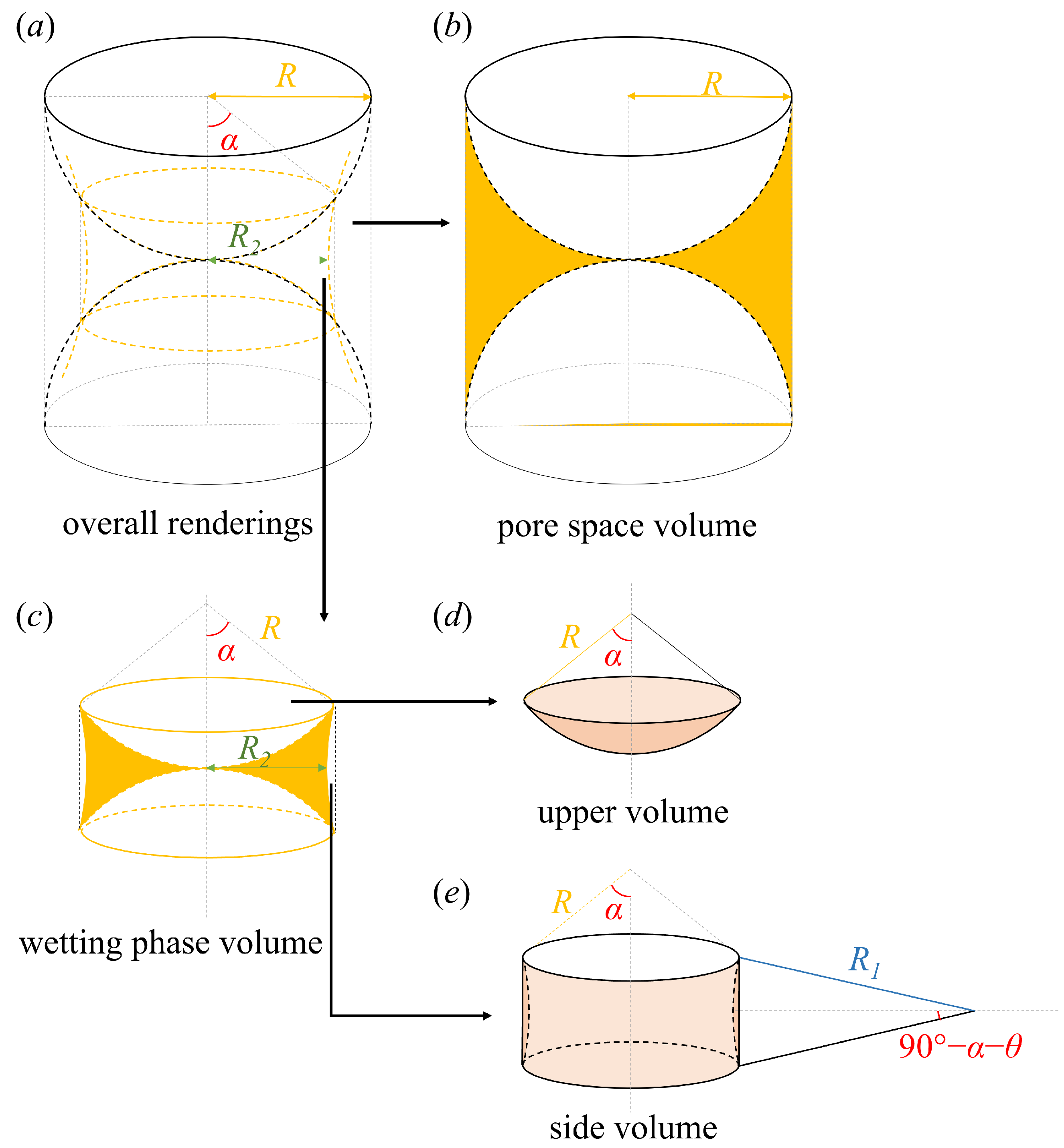
Equivalent Capillary Force

In this study, $F_c$ describes the force acting on proppants caused by multiphase flow, and $F_c$ is equal to the capillary force but in the opposite direction. $F_c$ is related to the parameters including interfacial tension, wetting angle ($\theta$), and included angle ($\alpha$). Fu [31] calculated these parameters by considering a 2D plane area. In this study, we determine $F_c$ by extending Fu’s [31] method to 3D space.

As illustrated in Figure 2e, proppants are surrounded by the wetting phase, and we determine the capillary pressure by the Young–Laplace Equation as follows [45]:

$$P_c=\sigma \left({\displaystyle \frac{1}{R_1}}-{\displaystyle \frac{1}{R_2}}\right)\times {10}^{-3}$$

(1)

where $\sigma$ is the interfacial tension, $\mathrm{m}\mathrm{N}/\mathrm{m}$; $R_1$ is the radius of the curved interface between wetting and non-wetting phases, m; and $R_1$ is related to the radius of proppant (R) and contact angle ($\theta$) by

$$R_1={\displaystyle \frac{R\left[\frac{1}{sin\left(\frac{\pi }{2}-\alpha \right)}-1\right]sin\left(\frac{\pi }{2}+\alpha \right)}{sin\left(\frac{\pi }{2}-\alpha -\theta \right)}}$$

(2)

where $\alpha$ describes the angle for the interface between fluids and proppant (see Figure 2e). $R_2$ is related to $R_1$ by

$$R_2=Rsin\alpha -R_1+R_{1}sin\left(\alpha +\theta \right)$$

(3)

Substituting $R_1$ and $R_2$ into Equation (1) determines $F_c$ as follows:

$$F_c=\sigma \left({\displaystyle \frac{1}{R_1}}-{\displaystyle \frac{1}{R_2}}\right)\times \pi {\left(Rsin\alpha \right)}^2$$

(4)

$\alpha$ is the primary unknown parameter in Equation (4). Below, we describe how to determine $\alpha$ in propped fracture in 3D space.

As shown in Figure 3b, in geometry, the volume of pore space $V_{pore}$ can be calculated by

$$V_{pore}={\displaystyle \frac{2}{3}}\pi R^3$$

(5)

The volume of the wetting phase in the pore space ($V_w$) is related to the porosity volume ($V_{pore}$) and saturation ($S_w$) by

$$V_w=V_{pore}\times S_w$$

(6)

$V_w$ can be determined by excluding the volume at the upper and lower cylinder ($V_2$) and the volume at the side of cylinder ($V_3$) from the cylinder volume ($V_1$) by

$$V_w=V_1-V_2-V_3$$

(7)

As illustrated by Figure 3c, $V_1$ is determined by

$$V_1=2\pi {\left(R·\sin \alpha \right)}^2{R}_1\sin \left({\displaystyle \frac{\pi }{2}}-\alpha -\theta \right)$$

(8)

$V_2$ is determined by the method of integration as follows (see Figure 3d):

$$V_2=2{\int }_{\alpha }^0\pi {\left(R\sin \beta \right)}^2\Delta h={\displaystyle \frac{4}{3}}\pi R^3-2\pi R^3\cos \alpha +{\displaystyle \frac{2}{3}}\pi R^3{\cos }^3\alpha$$

(9)

As illustrated by Figure 3e, $V_3$ is determined by the method of integration as follows:

$$\begin{array}{c}{V}_3={\int }_0^{{\displaystyle \frac{\pi }{2}}-\alpha -\theta }\Delta \pi {\left\{R-\left[R_1\cos \beta -R_1\cos \left({\displaystyle \frac{\pi }{2}}-\alpha -\theta \right)\right]\right\}}^2·h\hfill \\ =\pi R_1^2\left[R+R_1\cos \left({\displaystyle \frac{\pi }{2}}-\alpha -\theta \right)\right]\left[\pi -2\alpha -2\theta -\sin \left(\pi -2\alpha -2\theta \right)\right]-{\displaystyle \frac{4}{3}}\pi R_1^3{\sin }^3\left({\displaystyle \frac{\pi }{2}}-\alpha -\theta \right)\hfill \end{array}$$

(10)

Substituting Equations (8)–(10) into Equation (7) determines the volume of the wetting phase, and $\alpha$ is solved numerically through iterations. $F_c$ can be determined by substituting $\alpha$ and R into Equation (4).

Critical Velocity of Proppant Flowback

The proppant flowback is expected to occur at a critical flow velocity beyond which forces are no longer balanced. In other words, the proppant starts to move as the resisting forces acting on proppant become lower than dragging forces, which are expected to be a function of the fluids’ velocity. Here, we describe how to determine the critical velocity for proppant flowback before and after fracture closure, respectively.

(1)

Before fracture closure

During early flowback, the pressure in fractures may remain higher than closure pressure for wells with limited days of shut-in after fracturing treatment. The mainly acting forces include net gravity (G) and viscous dragging force ($F_{drag}$) considering the relatively loose arrangements of proppants before fracture closure (see Figure 2d). G is the property of proppants, and is quantified by

$$G={\displaystyle \frac{4}{3}}\pi R^{3}g\left({\rho }_s-{\rho }_l\right)\times {10}^{-12}$$

(11)

where ${\rho }_s$ is the proppant density, g/cm³, and ${\rho }_l$ is the fracturing fluid density, g/cm³.

The proppant is also subject to $F_{drag}$, which is caused by the difference in the velocity of the particles and fluid:

$$F_{drag}=C_d{\displaystyle \frac{\pi R^2{\rho }_l{v}^2}{2}}\times {10}^{-6}$$

(12)

where v is the flowback velocity, m/s; $C_d$ is the resistance coefficient, which is dimensionless; and $C_d$ is related to the Reynolds number (Re) by

$$C_d={\displaystyle \frac{24}{\mathrm{Re}}}\left(1+0.15{\mathrm{Re}}^{0.687}\right)\left(\mathrm{Re}\le 1000\right)$$

(13)

$$C_d=0.44\left(\mathrm{Re}>1000\right)$$

where Re is expressed by

$$\mathrm{Re}={\displaystyle \frac{{\rho }_l·2Rv}{\mu }}$$

(14)

where $\mu$ is the viscosity of the fracturing fluid, mPa·s.

Under the critical condition of proppant flowback, we thus mainly consider the torque equilibrium between G and $F_{drag}$ acting on proppants as follows:

$$G{L}_1=F_{drag}{L}_2$$

(15)

where $L_1$ and $L_2$ are determined by

$$L_1={\displaystyle \frac{1}{2}}R$$

$$L_2={\displaystyle \frac{\sqrt{3}}{2}}R$$

Combining the torque equilibrium and Reynold number results in the following expression for critical velocity:

$$v=\sqrt{{\displaystyle \frac{8·3^{\frac{1}{2}}Rg\left({\rho }_s-{\rho }_l\right)}{9C_d{\rho }_l}}\times {10}^{-6}}$$

(16)

(2)

After fracture closure

The pressure in fractures gradually drops below the closure pressure with pressure depletion during flowback. Considering the relatively tight arrangements of proppants in the fractures, we here include the bonding force ($F_{bond}$), friction force ($F_f$), down force of liquid ($F_{down}$), and $F_c$ in addition to G and $F_{drag}$ (see Figure 2d). $F_f$ is determined by

$$F_f={\displaystyle \frac{\sqrt{3}}{2}}{\mu }_f\pi R^2\Delta P\times {10}^{-9}$$

(17)

where $\Delta P$ is the net pressure in fractures, Pa, and ${\mu }_f$ is the friction coefficient, which is dimensionless.

$F_{down}$ is described by

$$F_{down}={\displaystyle \frac{\pi }{16}}{\rho }_{l}ghR\delta \times {10}^{-8}$$

(18)

where $\delta$ is the parameter describing the film formed between particles $\mathrm{c}\mathrm{m}$.

$F_{bond}$ is related to the radius of the proppant by

$$F_{bond}={\displaystyle \frac{\pi }{16}}R\epsilon \times {10}^{-6}$$

(19)

where $\epsilon$ is the coefficient of the bonding force, $\mathrm{d}\mathrm{y}\mathrm{n}/\mathrm{c}\mathrm{m}$.

The equilibrium of torque is then described by

$$\left(G+F_{down}+F_{bond}\right)L_1+F_f{L}_2=\left(F_{drag}+F_c\right)L_2$$

(20)

Combining the torque equilibrium and Reynold number results in the following expression for critical velocity:

$$v=\sqrt{{\displaystyle \frac{3^{\frac{1}{2}}{\mu }_f\Delta P\times {10}^{-3}-2\sigma {\sin }^2\alpha \left(\frac{1}{R_1}-\frac{1}{R_2}\right)\times {10}^6}{C_d{\rho }_l}}+{\displaystyle \frac{8·3^{\frac{1}{2}}Rg\left({\rho }_s-{\rho }_l\right)\times {10}^{-6}}{9C_d{\rho }_l}}+{\displaystyle \frac{3^{\frac{1}{2}}{\rho }_{l}gh\delta \times {10}^{-2}+3^{\frac{1}{2}}\epsilon }{24C_{d}R{\rho }_l}}}$$

(21)

2.1.2. Fracture Conductivity

According to the Carman–Kozeny formula, the fracture conductivity ($C_f$) is defined by

$$C_f=k_f{W}_f={\displaystyle \frac{\varphi r^2}{8{\tau }^2}}·W_f$$

(22)

where $k_f$ is the permeability of the propped fracture, ${\mathrm{m}}^2$; $W_f$ is the width of the propped fracture, m; $\varphi$ is the fracture porosity, which is dimensionless; r is the radius of the pore throat in the propped fracture, m; and $\tau$ is the tortuosity, which is dimensionless. In this study, we primarily modify Gao et al.’s [42] method to determine $\tau$ and r by considering the proppant flowback. Details about $W_f$, $\varphi$, $\tau$, and r are described below for the scenarios before and after fracture closure, respectively.

(1)

Before fracture closure

Before fracture closure, $W_f$ without any proppant embedment or deformation ($W_{f0}$) is related to R by

$$W_{f0}={\displaystyle \frac{2\sqrt{6}}{3}}\left(m-1\right)R+2R$$

(23)

where m corresponds to the total number of proppant layers, and m is related to the total number of proppants (N) by

$$m={\displaystyle \frac{N}{\left(\frac{L_f}{2R}\right)\left(\frac{H_f-2R}{\sqrt{3}R}+1\right)}}$$

(24)

where $L_f$ is the fracture half length, m, and $H_f$ is the fracture height, m.

Before fracture closure, the fracture porosity without any deformation and embedment (${\varphi }_0$) is 25.9%. The pore throat radius ($r_0$), which refers to the radius of the incircle between the particles, is related to R by $\left({\displaystyle \frac{2\sqrt{3}}{3}}-1\right)R$. The tortuosity (${\tau }_0$) refers to the ratio of the effective length of the curved channel to the shortest distance, and is set to ${\displaystyle \frac{\sqrt{6}}{2}}$.

(2)

After fracture closure

After fracture closure, the loss in fracture width ($\Delta W_f$) is mainly caused by proppant deformation and embedment as follows:

$$\Delta W_f=\Delta W_d+\Delta W_e$$

(25)

where $\Delta W_d$ and $\Delta W_e$ are the reduction in fracture width caused by proppant deformation and embedment, respectively. $\Delta W_d$ is related to the Poisson ratio and elastic modulus by

$$\Delta W_d=0.945W_{f0}{\left(\Delta P{\displaystyle \frac{1-{\nu }_1^2}{E_1}}\right)}^{{\displaystyle \frac{2}{3}}}$$

(26)

where $\Delta P$ is the net pressure in fractures, Pa; ${\nu }_1$ is the Poisson ratio of the proppant, which is dimensionless; and $E_1$ is the elastic modulus of the proppant, Pa.

Proppant embedment mainly occurs at the interface between the proppant and fracture surface, and $\Delta W_e$ is related to the Poisson ratio and elastic modulus by

$$\Delta W_e=1.89R\Delta P^{{\displaystyle \frac{2}{3}}}\left[{\left({\displaystyle \frac{1-{\nu }_1^2}{E_1}}+{\displaystyle \frac{1-{\nu }_2^2}{E_2}}\right)}^{{\displaystyle \frac{2}{3}}}-{\left({\displaystyle \frac{1-{\nu }_1^2}{E_1}}\right)}^{{\displaystyle \frac{2}{3}}}\right]$$

(27)

where ${\nu }_2$ is the Poisson ratio of formation, which is dimensionless, and $E_2$ is the formation elastic modulus, Pa. Substituting Equations (26) and (27) into Equation (25), we have

$$\Delta W_f=1.89R\Delta P^{{\displaystyle \frac{2}{3}}}\left[{\left({\displaystyle \frac{1-{\nu }_1^2}{E_1}}+{\displaystyle \frac{1-{\nu }_2^2}{E_2}}\right)}^{{\displaystyle \frac{2}{3}}}-{\left({\displaystyle \frac{1-{\nu }_1^2}{E_1}}\right)}^{{\displaystyle \frac{2}{3}}}+{\displaystyle \frac{W_{f0}}{2R}}{\left({\displaystyle \frac{1-{\nu }_1^2}{E_1}}\right)}^{{\displaystyle \frac{2}{3}}}\right]$$

(28)

By combining Equations (23) and (28), $W_f$ is expressed by

$$\begin{array}{c}{W}_f=\left({\displaystyle \frac{2\sqrt{6}R}{3}}+2R\right)\left[{\displaystyle \frac{N}{\left(\frac{L_f}{2R}\right)\left(\frac{H_f-2R}{\sqrt{3}R}+1\right)}}-1\right]\left[1-{\displaystyle \frac{1.89R\Delta P^{\frac{2}{3}}}{2R}}{\left({\displaystyle \frac{1-{\nu }_1^2}{E_1}}\right)}^{{\displaystyle \frac{2}{3}}}\right]\hfill \\ -1.89R\Delta P^{{\displaystyle \frac{2}{3}}}\left[{\left({\displaystyle \frac{1-{\nu }_1^2}{E_1}}+{\displaystyle \frac{1-{\nu }_2^2}{E_2}}\right)}^{{\displaystyle \frac{2}{3}}}-{\left({\displaystyle \frac{1-{\nu }_1^2}{E_1}}\right)}^{{\displaystyle \frac{2}{3}}}\right]\hfill \end{array}$$

(29)

In Equation (29), the fracture width decreases with decreasing N due to the proppant flowback.

By treating the pore throat as an ellipse transformed from a circle due to longitudinal compression, Gao et al. [42] approximately regarded the short radius of ellipse as r. As shown in Figure 4b, however, the pore throat between the ellipsoid is circular. We thus modify r by relating it to $\Delta W_e$ as follows:

$$r=\left(2-\sqrt{3}\right){\displaystyle \frac{R\sqrt{8{\left(R-\Delta W_d\right)}^2+R^2}}{\sqrt{3}R+2\sqrt{2{\left(R-\Delta W_d\right)}^2+R^2}}}$$

(30)

Similarly, we modify Gao et al.’s [42] expression for the tortuosity considering proppant deformation (see Figure 4c) by

$$\tau ={\displaystyle \frac{\sqrt{\frac{4}{3}{R}^2+\frac{1}{6}{\left(R-\Delta W_d\right)}^2}}{R}}$$

(31)

We assume that the decrease in pore space caused by deformation is proportional to the loss in proppant volume caused by proppant deformation, and thus assume negligible change in porosity $\varphi$. The fracture conductivity after considering deformation and embedment is further determined by substituting Equations (29)–(31) into Equation (22):

$$\begin{array}{c}{C}_f={\displaystyle \frac{21-12\sqrt{2}-12\sqrt{3}+7\sqrt{6}}{2}}{\displaystyle \frac{\varphi R^5\left(8R^{\prime 2}+R^2\right)}{{\left(\sqrt{3}R+2\sqrt{2R^{\prime 2}+R^2}\right)}^2\left(R^{\prime 2}+8R^2\right)}}\left[{\displaystyle \frac{N}{\left(\frac{L_f}{2R}\right)\left(\frac{H_f-2R}{\sqrt{3}R}+1\right)}}-1\right]\left[1-{\displaystyle \frac{1.89R\Delta P^{\frac{2}{3}}}{2R}}{\left({\displaystyle \frac{1-{\nu }_1^2}{E_1}}\right)}^{{\displaystyle \frac{2}{3}}}\right]\hfill \\ -{\displaystyle \frac{5.67{\left(2-\sqrt{3}\right)}^2}{4}}{\displaystyle \frac{\varphi R^5\Delta P^{\frac{2}{3}}\left(8R^{\prime 2}+R^2\right)}{{\left(\sqrt{3}R+2\sqrt{2R^{\prime 2}+R^2}\right)}^2\left(R^{\prime 2}+8R^2\right)}}\left[{\left({\displaystyle \frac{1-{\nu }_1^2}{E_1}}+{\displaystyle \frac{1-{\nu }_2^2}{E_2}}\right)}^{{\displaystyle \frac{2}{3}}}-{\left({\displaystyle \frac{1-{\nu }_1^2}{E_1}}\right)}^{{\displaystyle \frac{2}{3}}}\right]\hfill \end{array}$$

(32)

And $R^{\prime }$ is expressed by

$$R^{\prime }=R-\Delta W_d$$

(33)

2.2. Finite-Element Simulation

In this study, we build a finite-element model by COMSOL Multiphysics to simulate the process of proppant flowback in a single hydraulic fracture. We here describe the assumptions and modeling setups for the finite-element simulation.

2.2.1. Assumptions

(1) Considering a symmetrical fracture, we mainly simulate the process of proppant flowback in a half fracture plane.

(2) We mainly consider the proppants flowback in 2D space (see Figure 5) and ignore the tortuosity of propped fracture in this simulation.

(3) Fluid follows laminar flow in the fracture. We ignore the leak-off effects during the flowback process.

2.2.2. Mesh Geometry and Conditions

In this study, we simulate the proppant flowback process for a vertical well completed in a tight field.

Table 1. Key inputs for calculating the critical velocity for a well completed in a tight reservoir.

Parameters	Value
Half-length of the fracture, $L_f$ (m)	118.95
Fracture height, $H_f$ (m)	42
Volume of pumped proppant, $V_s$ (m3)	40
Proppant radius, R ($\mathsf{\mu }$m)	350
Proppant density, ${\rho }_s$ (g/cm3)	3.16
Volume density of proppant, ${\rho }_{vs}$ (g/cm3)	1.74
Fracturing fluid density, ${\rho }_l$ (g/cm3)	1.03
Fracturing fluid viscosity for gel breaking, $\mu$ (mPa·s)	3.5
Friction coefficient of quartz, ${\mu }_f$	0.75
Film parameter of quartz, $\delta$ (cm)	0.0000213
Bonding force coefficient of quartz, $\epsilon$ (dyne/cm)	2.56
Surface tension of gel breaking fracturing fluid, $\sigma$ (mN/m)	24.4
Wetting angle, $\theta$ (°)	2
Net pressure in fractures, $\Delta P$ (Pa)	1
Wetting-phase saturation in the fracture, $S_w$ (%)	14.7
Poisson’s ratio of proppant, ${\nu }_1$	0.25
Elastic modulus of proppant, $E_1$ (${10}^9$ Pa)	100
Poisson’s ratio of formation, ${\nu }_2$	0.19
Elastic modulus of formation, $E_2$ (${10}^9$ Pa)	34

lists the key inputs for the finite-element simulation. Here, we describe the key conditions for the simulation model of fluid and proppant flow within the fracture.

(1) Multiphysics: The simulation is built on the basis of the Laminar Flow physical field and the Particle Tracing for Fluid physical field [37].

(2) Mesh Geometry: Figure 5 shows the mesh setups for the finite-element model which simulates the proppant flowback process in the right-half fracture plane (see Figure 2b). We select triangular meshes for the model and refine the grids around perforation hole for better characterizations of the flow near the wellbore.

(3) Boundary: In the finite-element model, we set no-flow boundaries at the left, upper, and lower ends of fracture.

(4) Force: Proppants are randomly placed inside the fracture, and proppants are affected by gravity, viscous dragging force, friction force, down force, bonding force, and equivalent capillary force (see Figure 2d and Section 2.1.1).

3. Application and Results

In this section, we describe the field and well information for application. We then report the results of critical velocity and fracture conductivity obtained by analytical modeling, and also report the results of simulation for a base case. We further show the results of analytical modeling and simulation for the cases with varying saturation and net pressure in fractures.

3.1. Field and Well Information

The target well is a vertical well completed in the Shenfu Block, which is a tight reservoir in the Ordos Basin. Table 1 lists the key hydraulic-fracturing parameters for the target well. During hydraulic fracturing, the well is pumped with 40 m³ of proppants (mainly quartz). Table 1 provides the properties of the proppant, including the proppant radius, the proppant density, the Poisson ratio of the proppant, and the elastic modulus. In Table 1, we also list the density and viscosity of the fracturing fluid (guar gum). Additionally, the target formation is characterized with an elastic modulus of 34 GPa and a Poisson ratio of 0.19.

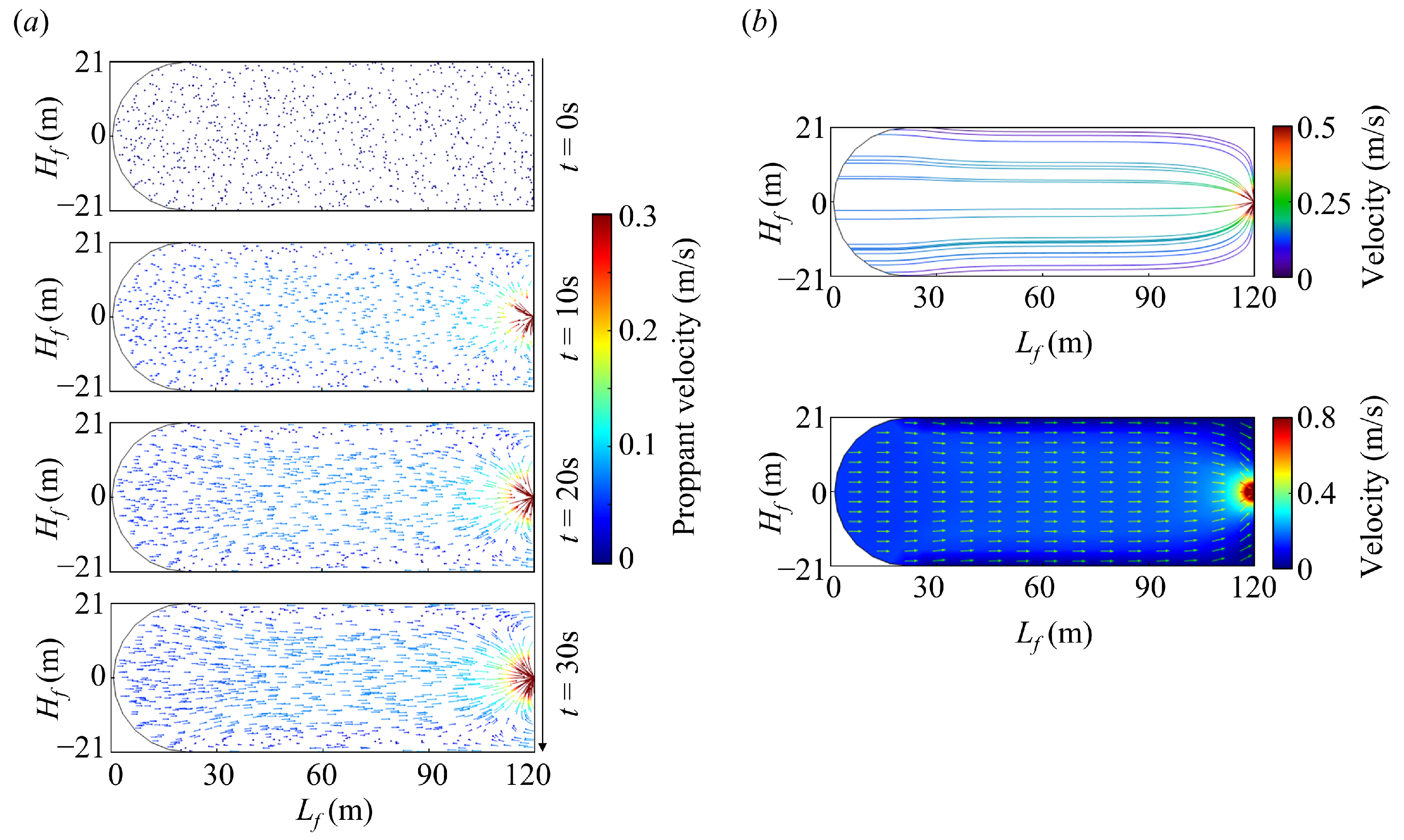
3.2. Results of Base Case

By substituting the parameters for the base case into Equations (16) and (21), we obtain the critical velocity of 0.0529 and 0.0591 m/s for the proppant flowback before and after fracture closure, respectively. Figure 6 shows the simulation results for the base case at a flowback velocity of 0.14 m/s, which is higher than the critical velocity for proppant flowback. We note that a total number of 1000 proppants are randomly distributed in the fracture at the onset of simulation, considering the computation costs for a large amount of proppants. As shown in Figure 6a,b, the proppant particles migrate along with direction of fluid flow, and accumulate around the perforation. The target well is pumped with 40 m³ of proppants. The simulation results show that a total number of 33 proppants (among 1000 proppants) are recovered through perforation. Accordingly, the remaining proppants are estimated to be 38.68 m³ at 30 s after fracture closure.

Before fracture closure, the fracture conductivity is calculated to be 0.1965 μm²·m (refer to Section 2.1.2) for the target well when the flowback velocity is lower than the critical value. Comparatively, the fracture conductivity is calculated to be 0.1903 μm²·m at 30 s after fracture closure when a flowback velocity of 0.14 m/s is employed.

3.3. The Effects of Water Saturation in Fractures

3.3.1. Critical Velocity

In Figure 7a, we compare the critical velocity of the proppant flowback with and without considering $F_c$. Note that we set $\Delta P$ = 1000 Pa at varying $S_w$. The results show a higher critical velocity calculated by our proposed model compared with Fu’s [31] model. The difference between the two models is relatively more significant at a relatively low $S_w$. One may thus expect that Fu’s [31] model, which builds on a 2D assumption, may underestimate the critical velocity for the proppant flowback, especially at late flowback.

In Figure 7a, the results of the models considering $F_c$ show an increasing v with $S_w$, until a constant v is reached. The results show a consistent value of v for the models with and without considering $F_c$ at $S_w$ > 0.28. Figure 7b shows a decreasing $F_c$ with increasing $S_w$ until $F_c$ reaches 0, corresponding to the increasing trends in v for the models considering $F_c$. The effects of $F_c$ are thus expected to be negligible on critical velocity at early flowback when $S_w$ remains high.

Figure 7c compares the critical velocity for the proppant radius varying from 250 to 350 $\mathsf{\mu }$m at a relatively low $S_w$. The results show an increasing critical velocity with increasing proppant radius. According to Equation (4), $F_c$ increases with increasing the proppant radius. However, we expect that the increase in the gravity of proppant is more significant than the increase in $F_c$, leading to a higher critical velocity for proppant flowback.

Figure 7d compares the critical velocity for $\theta$ varying from 2° to 60°. The results show that the critical velocity increases rapidly within a smaller range of variation at a relatively high $\theta$. $F_c$ plays a relatively important role at a low $S_w$, and $F_c$ is thus more sensitive to $S_w$. One may expect that $F_c$ has a greater effect on proppant particles with smaller $\theta$ at late flowback.

3.3.2. Proppant Flowback Volume and Fracture Conductivity

Figure 8a shows the change in proppant flowback volume during flowback at varying $S_w$. The proppant flowback volume increases with time, and generally increases with decreasing $S_w$. Decreasing $S_w$ increases $F_c$, which is a driving force for proppant movement. The increase in proppant flowback volume becomes less significant at a relatively higher $S_w$.

Figure 8b compares the change in $C_f$ with $S_w$ which varies from 0.1 to 0.147. Note that we set the range of $S_w$ at 0.1 to 0.147 by considering the results that the critical velocity does not change significantly beyond 0.147 (see Figure 7a). Overall, the results show a decreasing $C_f$ with proppant flowback. Also, the decrease in $C_f$ is relatively more significant at a lower $S_w$. Comparatively, the change in $S_w$ at a relatively higher value is associated with a more significant change in $C_f$. According to Equation (22), $C_f$ is mainly related to $W_f$, $\Delta W_d$, and $\Delta W_e$. $\Delta W_d$ and $\Delta W_e$ are constant at a consistent value of net pressure in fractures (see Equations (26) and (27). $W_f$ is then mainly determined by the proppant remaining in the fracture. Increasing $S_w$ contributes to a higher $W_f$ and $C_f$ because of the decreased proppant flowback. Moreover, the loss in fracture closure can also be resisted by the remaining water in the fracture, considering the relatively high water compressibility [46,47]. A higher $S_w$ may thus also resist the process of fracture closure.

Figure 8c shows the simulated fields of proppant velocity in hydraulic fracture at 30 s after fracture closure for four cases with $S_w$ varying from 0.1 to 0.147. Overall, the results show a relatively higher proppant velocity at a lower $S_w$. Also, a relatively larger portion of proppants show movements at lower $S_w$. At a higher $S_w$, the movement of the proppants is mainly constrained in the near-wellbore region, while the movement of proppants can be significant at the edge of the hydraulic fracture at a lower $S_w$. This highlights that the movement of the proppant can be relatively more significant at a relatively low water saturation in fractures.

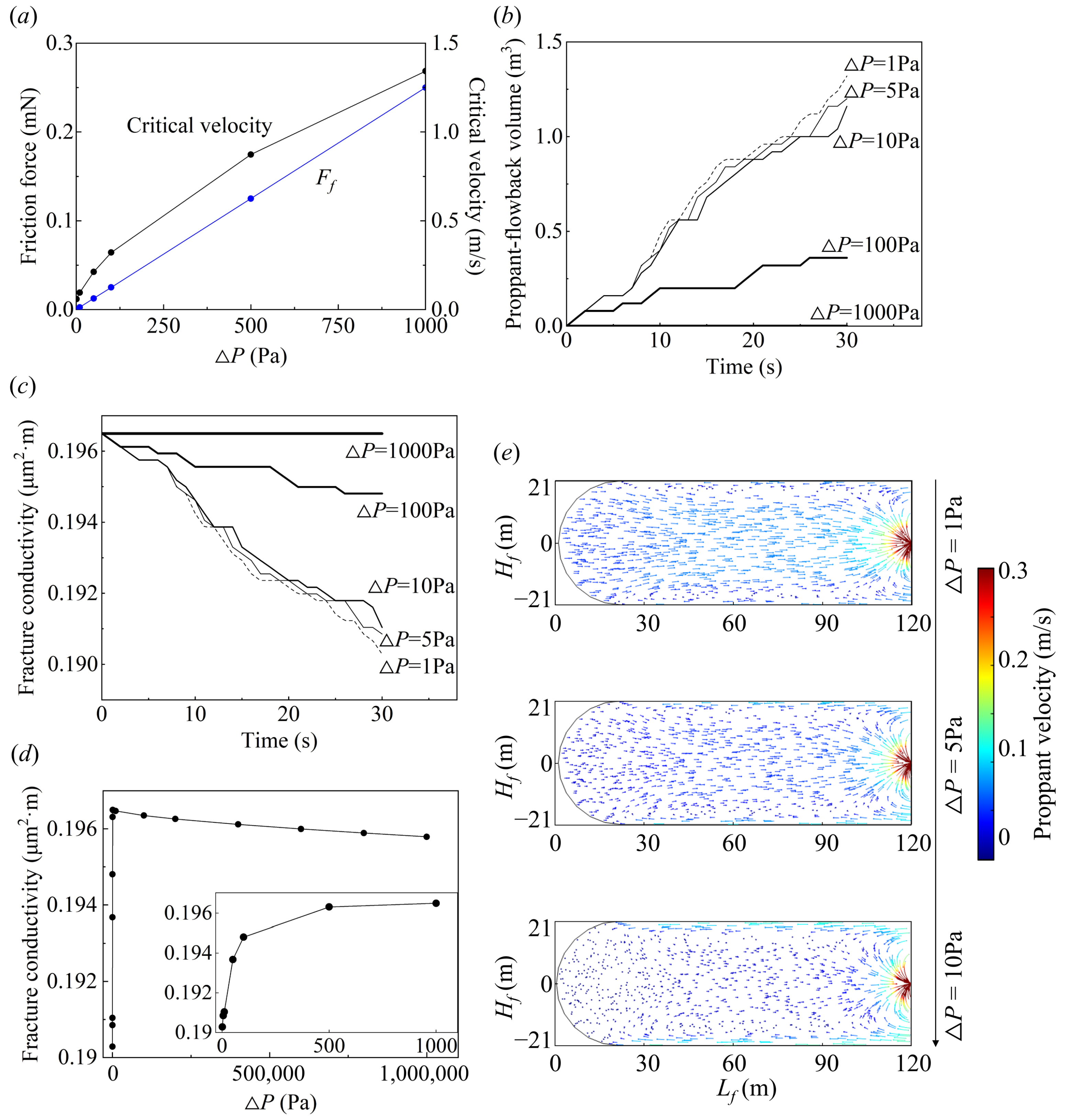
3.4. The Effects of Net Pressure in Fractures

3.4.1. Critical Velocity

Figure 9a plots the friction force and critical velocity as a function of the net pressure in fractures. Overall, the friction force and critical velocity increase with the net pressure in fractures. The results show a linear increase in friction force but a non-linear increase in critical velocity with net pressure in fractures, which are consistent with the relationships described by Equations (17) and (21).

We quantitatively compare the forces acting on the proppants with net pressure in fractures increasing from 1 to 1000 Pa, and our results show the friction force (0 to 0.25 mN) is of several magnitudes larger than the equivalent capillary force (0 to 0.0049 mN), net gravity force (3.75 $\times {10}^{-3}$ mN), down force (1.759 $\times {10}^{-5}$ mN), and bonding force (9.6 $\times {10}^{-9}$ mN). The results indicate that the dragging force created by the viscous flow of fracturing fluid is mainly balanced by friction force at the relatively high net pressure in fractures. In other words, the well can be operated at a relatively high flowback velocity at the late stage of flowback when the net pressure in fractures becomes relatively high.

3.4.2. Proppant Flowback Volume and Fracture Conductivity

Figure 9b compares the proppant flowback volume for the simulated cases with the net pressure in fractures varying from 1 to 1000 Pa. We note that a flowback velocity of 0.14 m/s is applied for these cases. The results show a decreasing proppant flowback volume with increasing net pressure in fractures, and the proppant flowback does not occur when the net pressure in fractures reaches 1000 Pa. These results highlight the importance of drawdown managements for preventing proppant flowback in the field [7,48,49].

Figure 9c plots the loss in fracture conductivity versus time for five cases with net pressure in fractures varying from 1 to 1000 Pa. We note that a constant net pressure in fractures was maintained for these five cases. The results show a consistent loss in fracture conductivity for these cases of 1 to 100 Pa, while the fracture conductivity generally remains constant for the case of 1000 Pa. Figure 9d plots the fracture conductivity versus net pressure in fractures. The results show a significant increase in fracture conductivity as the net pressure in fractures increases from 0 to 1000 Pa, and fracture conductivity slightly decreases with net pressure in fractures afterward.

The early significant change in the fracture conductivity with net pressure in fractures is mainly related to the proppant flowback. The proppant flowback volume decreases from 1.32 to 0 m³ as the net pressure in fractures increases from 0 to 1000 Pa. Meanwhile, the change in fracture width caused by deformation and embedments is only 0.0305 nm in total, which can be negligible. One may further conclude that the loss in fracture conductivity is more likely related to the proppant flowback rather than proppant deformation and embedments at early flowback. The late slight decrease in fracture conductivity is expected to be mainly caused by proppant deformation and embedments because no proppant flowback occurs at a flowback velocity of 0.14 m/s after the net pressure in fractures reaches 1000 Pa. At $\Delta P$ = 10⁶ Pa, $\Delta W_d$ and $\Delta W_e$ reach 1.3 nm and 1.75 nm, corresponding to 0.3% and 0.5% of proppant radius, respectively.

Figure 9e compares the fields of proppant velocity in hydraulic fracture with net pressure in fractures. The proppant movements become relatively more pronounced as net pressure in fractures decreases. Proppants in fractures at around 90 m away from perforation hole are involved with the proppant movement at the net pressure in fractures of 1 Pa. At a relatively high net pressure in fractures, the results show a relatively limited near-wellbore region with proppant movements.

4. Summary and Conclusions

This work established analytical models for determining the critical flowback velocity for proppant flowback, and assessed the loss in fracture conductivity caused by proppant flowback by combining the analytical model and finite-element simulation. The key findings can be summarized as follows:

(1) The critical velocity of proppant flowback before fracture closure is less than that after fracture closure. The friction force plays an important role in the increase of critical velocity.

(2) The multiphase effects on critical velocity of proppant flowback can be negligible at early flowback. Comparatively, the critical velocity is positively correlated with the saturation of the wetting phase ($S_w$) at late flowback. Increasing the proppant size increases the critical velocity, and increasing the contact angle leads to a sharp increase in the critical velocity over a relatively small interval of $S_w$. The volume of the proppant flowback increases with decreasing $S_w$, contributing to the loss in fracture conductivity.

(3) The critical velocity is positively correlated with the net pressure in fractures, whereas the volume of the proppant flowback is negatively correlated with the net pressure in fractures. The fracture conductivity initially increases and then decreases with the net pressure in fractures. The early increasing fracture conductivity is mainly related to the proppant flowback at relatively low net pressure in fractures, while the late decreasing fracture conductivity is mainly related to proppant deformation and embedments at high net pressure in fractures.

References

1. Li, Q.; Wang, Y.; Wang, F.; Wu, J.; Tahir, M.U.; Li, Q.; Yuan, L.; Liu, Z. Effect of thickener and reservoir parameters on the filtration property of CO2 fracturing fluid. Energy Sources Part A Recover. Util. Environ. Eff. 2020, 42, 1705–1715. [Google Scholar] [CrossRef]
2. Li, Q.; Liu, J.; Wang, S.; Guo, Y.; Han, X.; Li, Q.; Cheng, Y.; Dong, Z.; Li, X.; Zhang, X. Numerical insights into factors affecting collapse behavior of horizontal wellbore in clayey silt hydrate-bearing sediments and the accompanying control strategy. Ocean Eng. 2024, 297, 117029. [Google Scholar] [CrossRef]
3. Howard, P.R.; King, M.T.; Morris, M.; Feraud, J.-P.; Slusher, G.; Lipari, S. Fiber/proppant mixtures control proppant flowback in south texas. In Proceedings of the SPE Annual Technical Conference and Exhibition, Dallas, TX, USA, 22–25 October 1995. [Google Scholar]
4. Mayerhofer, M.J.; Wolhart, S.L.; Rogers, J.D. Results of U.S. department of energy deep gas well stimulation study. In Proceedings of the SPE Annual Technical Conference and Exhibition, Dallas, TX, USA, 9–12 October 2005. [Google Scholar]
5. Campos, M.; Potapenko, D.; Moncada, K.; Krishnamurthy, J. Advanced flowback in the powder river basin: Securing stimulation investments. In Proceedings of the SPE/AAPG/SEG Unconventional Resources Technology Conference, Denver, CO, USA, 22–24 July 2019; OnePetro: Richardson, TX, USA, 2019. [Google Scholar]
6. Chuprakov, D.; Belyakova, L.; Iuldasheva, A.; Alekseev, A.; Syresin, D.; Chertov, M.; Spesivtsev, P.; Suarez, F.I.S.; Velikanov, I.; Semin, L.; et al. Proppant flowback: Can we mitigate the risk? In Proceedings of the SPE Hydraulic Fracturing Technology Conference and Exhibition, The Woodlands, TX, USA, 4–6 February 2020; OnePetro: Richardson, TX, USA, 2020. [Google Scholar]
7. Fu, Y.; Dehghanpour, H.; Motealleh, S.; Lopez, C.M.; Hawkes, R. Evaluating fracture volume loss during flowback and its relationship to choke size: Fastback vs. slowback. SPE Prod. Oper. 2019, 34, 615–624. [Google Scholar] [CrossRef]
8. Potapenko, D.I.; Williams, R.D.; Desroches, J.; Enkababian, P.; Theuveny, B.; Willberg, D.M.; Moncada, K.; Deslandes, P.; Wilson, N.; Neaton, R.; et al. Securing long-term well productivity of horizontal wells through optimization of postfracturing operations. In Proceedings of the SPE Annual Technical Conference and Exhibition, San Antonio, TX, USA, 9–11 October 2017; OnePetro: Richardson, TX, USA, 2017. [Google Scholar]
9. Canon, J.M.; Romero, D.J.; Pham, T.T.; Valko, P.P. Avoiding proppant flowback in tight-gas completions with improved fracture design. In Proceedings of the SPE Annual Technical Conference and Exhibition, Denver, CO, USA, 3–4 October 2003. [Google Scholar]
10. Guo, S.; Wang, B.; Li, Y.; Hao, H.; Zhang, M.; Liang, T. Impacts of proppant flowback on fracture conductivity in different fracturing fluids and flowback conditions. ACS Omega 2022, 7, 6682–6690. [Google Scholar] [CrossRef] [PubMed]
11. James, S.G.; Samuelson, M.L.; Reed, G.W.; Sullivan, S.C. Proppant flowback control in high temperature wells. In Proceedings of the 1998 SPE Rocky Mountain Regional/Low-Permeability Reservoirs Symposium and Exhibition, Denver, CO, USA, 5–8 April 1998. [Google Scholar]
12. Bagci, S.; Stolyarov, S. Flowback production optimization for choke size management strategies in unconventional wells. In Proceedings of the SPE Annual Technical Conference and Exhibition, Calgary, AB, Canada, 30 September–2 October 2019; OnePetro: Richardson, TX, USA, 2019. [Google Scholar]
13. Deen, T.; Daal, J.; Tucker, J. Maximizing well deliverability in the eagle ford shale through flowback operations. In Proceedings of the SPE Annual Technical Conference and Exhibition, Houston, TX, USA, 28–30 September 2015; OnePetro: Richardson, TX, USA, 2015. [Google Scholar]
14. Karantinos, E.; Sharma, M.M.; Ayoub, J.A.; Parlar, M.; Chanpura, R.A. Choke-management strategies for hydraulically fractured wells and frac-pack completions in vertical wells. SPE Prod. Oper. 2018, 33, 623–636. [Google Scholar] [CrossRef]
15. Rojas, D.; Lerza, A. Horizontal well productivity enhancement through drawdown management approach in vaca muerta shale. In Proceedings of the SPE Canada Unconventional Resources Conference, Calgary, AB, Canada, 15–16 March 2018; OnePetro: Richardson, TX, USA, 2018. [Google Scholar]
16. Wilson, K.; Ahmed, I.; MacIvor, K. Geomechanical modeling of flowback scenarios to establish best practices in the midland basin horizontal program. In Proceedings of the SPE/AAPG/SEG Unconventional Resources Technology Conference, San Antonio, TX, USA, 1–3 August 2016; OnePetro: Richardson, TX, USA, 2016. [Google Scholar]
17. Shor, R.J.; Sharma, M.M. Reducing proppant flowback from fractures: Factors affecting the maximum flowback rate. In Proceedings of the SPE Hydraulic Fracturing Technology Conference, The Woodlands, TX, USA, 4–6 February 2014; OnePetro: Richardson, TX, USA, 2014. [Google Scholar]
18. Wang, Z.; Wang, X.; Shan, W.; Lu, Y. Development and research on fracturing technology in low-permeability ultra-deep wells in china. In Proceedings of the SPE Asia Pacific Oil and Gas Conference and Exhibition, Brisbane, Australia, 16–18 October 2000. [Google Scholar]
19. Daneshy, A. Proppant distribution and flowback in off-balance hydraulic fractures. SPE Prod. Facil. 2005, 20, 41–47. [Google Scholar] [CrossRef]
20. Milton-Tayler, D.; Stephenson, C.; Asgian, M.I. Factors affecting the stability of proppant in propped fractures: Results of a laboratory study. In Proceedings of the Society of Petroleum Engineers SPE Annual Technical Conference and Exhibition, Washington, DC, USA, 4–7 October 1992. [Google Scholar]
21. Wang, H.; Wen, L. Experimental investigation on the factors affecting proppant flowback performance. J. Energy Resour. Technol. Trans. ASME 2020, 142, 053001. [Google Scholar] [CrossRef]
22. Chun, T.; Zhu, D.; Zhang, Z.; Mao, S.; Wu, K. Experimental study of proppant transport in complex fractures with horizontal bedding planes for slickwater fracturing. SPE Prod. Oper. 2021, 36, 83–96. [Google Scholar] [CrossRef]
23. Chuprakov, D.; Iuldasheva, A.; Alekseev, A. Criterion of proppant pack mobilization by filtrating fluids: Theory and experiments. J. Pet. Sci. Eng. 2021, 196, 107792. [Google Scholar] [CrossRef]
24. Garagash, I.A.; Osiptsov, A.A.; Boronin, S.A. Dynamic bridging of proppant particles in a hydraulic fracture. Int. J. Eng. Sci. 2019, 135, 86–101. [Google Scholar] [CrossRef]
25. Stephenson, C.J.; Rickards, A.R.; Brannon, H.D. Increased resistance to proppant flowback by adding deformable particles to proppant packs tested in the laboratory. In Proceedings of the 1999 SPE Annual Technical Conference and Exhibition: ‘Drilling and Completion’, Houston, TX, USA, 3–6 October 1999. [Google Scholar]
26. Hu, J.; Zhao, J.; Li, Y. A proppant mechanical model in postfrac flowback treatment. J. Nat. Gas Sci. Eng. 2014, 20, 23–26. [Google Scholar] [CrossRef]
27. Richefeu, V.; Youssoufi, M.S.E.; Radjaï, F. Shear strength properties of wet granular materials. Phys. Rev. E—Stat. Nonlinear Soft Matter Phys. 2006, 73, 051304. [Google Scholar] [CrossRef] [PubMed]
28. Wang, K.; Zhang, M.; Wang, B.; Shi, J. A proppant flowback mechanical model based on different wettability of the proppant particle surface. In Proceedings of the International Field Exploration and Development Conference 2020; Springer: Singapore, 2021; pp. 3374–3384. [Google Scholar]
29. Wang, M.; Guo, B. Effect of fluid contact angle of oil-wet fracture proppant on the competing water/oil flow in sandstone-proppant systems. Sustainability 2022, 14, 3766. [Google Scholar] [CrossRef]
30. Zhou, Y.; Ni, H.; Shen, Z.; Wang, M. Study on proppant transport in fractures of supercritical carbon dioxide fracturing. Energy Fuels 2020, 34, 6186–6196. [Google Scholar] [CrossRef]
31. Fu, Y. Study on Proppant Backflow Mechanism during the Production Process of Fracturing Gas Well; Southwest Petroleum University: Chengdu, China, 2006. [Google Scholar]
32. Han, G.; Dusseault, M.B.; Cook, J. Quantifying rock capillary strength behavior in unconsolidated sandstones. In Proceedings of th SPE/ISRM Rock Mechanics Conference, Irving, TX, USA, 20–23 October 2002. [Google Scholar]
33. Han, G.; Dusseault, M.B. Quantitative analysis of mechanisms for water-related sand production. In Proceedings of the SPE International Symposium and Exhibition on Formation Damage Control, Lafayette, LA, USA, 20–21 February 2002. [Google Scholar]
34. Liu, Y.; Leung, J.Y.; Chalaturnyk, R. Geomechanical simulation of partially propped fracture closure and its implication for water flowback and gas production. SPE Reserv. Eval. Eng. 2018, 21, 273–290. [Google Scholar] [CrossRef]
35. Boyer, F.; Guazzelli, E.; Pouliquen, O. Unifying suspension and granular rheology. physical review letters. Phys. Rev. Lett. 2011, 107, 188301. [Google Scholar] [CrossRef] [PubMed]
36. Lecampion, B.; Garagash, D.I. Confined flow of suspensions modelled by a frictional rheology. J. Fluid Mech. 2014, 759, 197–235. [Google Scholar] [CrossRef]
37. Cao, G.; Bai, Y.; Du, T.; Yang, T.; Yan, H. Study on proppant backflow based on finite element simulation. Xinjiang Pet. Geol. 2019, 40, 10–12. [Google Scholar]
38. Dontsov, E.V.; Peirce, A.P. Slurry flow, gravitational settling and a proppant transport model for hydraulic fractures. J. Fluid Mech. 2014, 760, 567–590. [Google Scholar] [CrossRef]
39. Vega, F.G.; Carlevaro, C.M.; Sánchez, M.; Pugnaloni, L.A. Stability and conductivity of proppant packs during flowback in unconventional reservoirs: A cfd—dem simulation study. J. Pet. Sci. Eng. 2021, 201, 108381. [Google Scholar] [CrossRef]
40. Wang, J.; Elsworth, D.; Denison, M.K. Propagation, proppant transport and the evolution of transport properties of hydraulic fractures. J. Fluid Mech. 2018, 855, 503–534. [Google Scholar] [CrossRef]
41. Kozeny, J.; Carmen, P.C. Ueber kapillare leitung des wassers im boden sitzungsber akad. Wien 1927, 136, 271–306. [Google Scholar]
42. Gao, Y.; Lv, Y.; Wang, M.; Li, K. New mathematical models for calculating the proppant embedment and fracture conductivity. In Proceedings of theSPE Annual Technical Conference and Exhibition, San Antonio, TX, USA, 8–10 October 2012. [Google Scholar]
43. Jia, L.; Li, K.; Zhou, J.; Yan, Z.; Wan, F.; Kaita, M. A mathematical model for calculating rod-shaped proppant conductivity under the combined effect of compaction and embedment. J. Pet. Sci. Eng. 2019, 180, 11–21. [Google Scholar] [CrossRef]
44. Meng, Y.; Li, Z.; Guo, Z. Calculation model of fracture conductivity in coal reservoir and its application. J. China Coal Soc. 2014, 39, 1852–1856. [Google Scholar]
45. Leverett, M.C. Capillary behavior in porous solids. Trans. AIME 1941, 142, 152–169. [Google Scholar] [CrossRef]
46. Ehlig-Economides, C.A.; Economides, M.J. Water as proppant. In Proceedings of the SPE Annual Technical Conference and Exhibition, Denver, CO, USA, 30 October–2 November 2011; OnePetro: Richardson, TX, USA, 2011. [Google Scholar]
47. Fu, Y.; Dehghanpour, H.; Ezulike, D.O.; Jones, R.S., Jr. Estimating effective fracture pore volume from flowback data and evaluating its relationship to design parameters of multistage-fracture completion. SPE Prod. Oper. 2017, 32, 423–439. [Google Scholar] [CrossRef]
48. Almasoodi, M.; Vaidya, R.; Reza, Z. Drawdown-management and fracture-spacing optimization in the meramec formation: Numerical-and economics-based approach. SPE Reserv. Eval. Eng. 2020, 23, 1251–1264. [Google Scholar] [CrossRef]
49. Mirani, A.; Marongiu-Porcu, M.; Wang, H.; Enkababian, P. Production-pressure-drawdown management for fractured horizontal wells in shale-gas formations. SPE Reserv. Eval. Eng. 2018, 21, 550–565. [Google Scholar] [CrossRef]
Figure 1. Flow chart for calculating the critical velocity and the fracture conductivity considering proppant flowback.
Energies 17 04250 g001
Figure 2. Schematics illustrating the physical model of proppant flowback after the fracturing treatment of a multifractured horizontal well: (a) Schematics showing the concepts of a multifractured horizontal well, where the wellbore is intersected by multiple plane fractures. (b) The side view of plane fractures from the right, illustrating the concepts of fracture half-length ( L f ) and fracture height ( H f ). (c) The vertical view of plane fractures from the front, illustrating proppant settlements before and after fracture closure. (d) Schematics showing the 6 types of forces acting on proppants during flowback. These forces include net gravity force (G), viscous dragging force ( F d r a g ), friction force ( F f ), down force ( F d o w n ), bonding force between proppants ( F b o n d ), and equivalent capillary force ( F c ). The directions of forces are marked by arrows using different colors. (e) Geometric diagram illustrating the concepts for the descriptions of equivalent capillary force.
Energies 17 04250 g002
Figure 3. Geometric diagram illustrating the pore space and wetting fluid between two proppants, which are treated as two spherical particles: (a) The radii of curvature and shape of wetting phase held in pendular space between two proppants. (b) The geometry of pore space with a volume of V p o r e . (c) The distribution of wetting phase V w . (d) Schematics showing the volume of upper cylinder ( V 2 ). (e) Schematics showing the side view of cylinder with a volume of V 3 . The parameters including the proppant particle radius (R), contact angle ( θ ), radius of curved interface ( R 1 , R 2 ), and angle relating to wetting phase saturation ( α ) are also illustrated here.
Energies 17 04250 g003
Figure 4. Geometrics illustrating how the pore throat radius (r) and tortuosity ( τ ) are determined: (a) Schematic diagram of tightly arranged ellipsoidal proppants with deformation being considered. (b) r is determined by the radius of tangent circle between ellipsoidal particles. (c) τ is determined by the ratio of the effective curved channel ( 2 O N ) to the shortest distance ( M N ).
Energies 17 04250 g004
Figure 5. Geometry, dimensions, and meshing schematics for the finite-element model which simulates the proppant flowback process in a half fracture plane. The meshes are refined for the grids surrounding the perforated hole.
Energies 17 04250 g005
Figure 6. The results of the simulation for the base case when a flowback velocity (0.14 m/s) higher than critical value (0.0591 m/s) i semployed: (a) The distribution of proppants in the hydraulic fracture at the time of 0 to 30 s after fracture closure. The color gradient demonstrates the proppant velocity. (b) The velocity field of proppant (up) and fracturing fluid (low) at 30 s after fracture closure.
Energies 17 04250 g006
Figure 7. (a) Comparing the critical velocity of the proppant flowback as a function of S w calculated by the proposed model, Fu’s [31] model, and the model without considering multiphase effects. (b) Comparing the equivalent capillary force calculated by our proposed model and Fu’s [31] model. (c) The critical velocity calculated by the proposed model as a function of S w for proppant radius varying from 250 to 350 μ m. (d) The critical velocity calculated by the proposed model as a function of S w for contact angle varying from 2° to 60°.
Energies 17 04250 g007
Figure 8. Comparing the (a) proppant flowback volume, (b) fracture conductivity, and (c) fields of proppant velocity at 30 s after fracture closure with S w varying from 0.1 to 0.147. Note that a flowback velocity of 0.14 m/s was applied for the simulation. The proppant velocity is highlighted by the color gradient.
Energies 17 04250 g008
Figure 9. Comparatively analysis illustrating the effects of net pressure in fractures on critical velocity, proppant flowback volume, and fracture conductivity. A flowback velocity of 0.14 m/s was applied for the simulation: (a) the critical velocity and friction force as a function of net pressure in fractures; (b) the proppant flowback volume at net pressure in fractures varying from 1 to 1000 Pa; (c) comparing fracture conductivity with net pressure in fractures (varying from 0 to 106 Pa); (d) the loss in fracture conductivity as a function of time for net pressure in fractures varying from 1 to 1000 Pa; (e) comparing the fields of proppant velocity at 30 s of simulation with net pressure in fractures (from 1 to 10 Pa). Color gradient illustrates the distribution of proppant velocity.
Energies 17 04250 g009