Electric-Thermal Analysis of Power Supply Module in Graphitization Furnace

Abstract

Graphite, a key anode material in lithium-ion batteries, primarily relies on the Acheson graphitization furnace (AGF) for production. This research focuses on the power supply module of the AGF, particularly the electrodes and their power transmission clamps. A three-dimensional transient electric-thermal-fluid coupling model was developed to numerically analyze the temperature and electric field distributions during operation. The study revealed that heat conduction through furnace electrodes dominates temperature rise. Notably, clamping plates within transmission clamps exhibit high temperatures and gradients, posing a thermal failure risk. Efficient cooling plate design with liquid-cooled channels is crucial for temperature control. Additionally, maintaining high electrode temperatures reduces resistivity, lowering power consumption in the power supply module. This study provides insights into optimizing AGF power supply module design, emphasizing the importance of effective cooling strategies for clamping plates and the benefits of maintaining elevated electrode temperatures for energy efficiency.

1. Introduction

Due to its outstanding advantages of high energy density, high power density, long cycle life, and environmental friendliness, lithium-ion batteries have been widely applied in digital products, electric tools, transportation, and power energy storage facilities, driving the vigorous development of upstream and downstream industries [1,2,3,4,5,6,7]. Among the mainstream lithium-ion battery technologies in the current industry, various cathode materials are available, such as lithium iron phosphate (LFP) and nickel–cobalt–manganese (NCM) ternary materials, while graphite has consistently dominated the anode material market [8,9,10]. This is attributed to graphite’s array of benefits, including high electric conductivity, high thermal conductivity, high crystallinity, low thermal expansion, and resistance to high temperatures and corrosion [11]. Initially, the industry primarily utilized natural graphite as the anode material for lithium-ion batteries. However, with the soaring demand for lithium-ion batteries in recent years, the reserves of natural graphite are decreasing, prompting a significant shift to the use of synthetic graphite [12,13,14]. Synthetic graphite is usually produced from raw materials like anthracite, coke, or petroleum coke through processes such as crushing, mixing with coal tar oil and pitch, extrusion or molding, and finally calcination in an electric furnace under airtight conditions [15,16]. Currently, the primary equipment for calcining graphite is the Acheson graphitization furnace (AGF) [17].

AGF achieves graphite calcination by passing electric current through the resistive material in the furnace core, generating heat, and then heating the graphite calcination product through heat transfer to complete the graphitization process [18]. While AGF is widely used due to its large capacity and simple structure, it faces critical issues such as low-capacity utilization, high power consumption, and failure rates, as well as quality fluctuations caused by uneven current and temperature distributions, as it is a batch-type furnace with periodic production [19,20,21]. According to statistics, the total energy consumption for producing one ton of graphite material is as high as 5–6 tons of standard coal, which accounts for more than 30% of the total production cost. The power consumption of the graphitization procedure in the AGF accounts for about 70% of the total energy consumption in the whole production process [22]. Thus, improving the energy efficiency index of the graphitization procedure is a key link to reducing the cost of graphite generation and improving economic benefits.

To enhance the operational efficiency and product quality in AGFs, numerous scholars have conducted extensive research from the perspectives of structural optimization, material screening, and power transmission process design and control. Shang et al. [23] predicted the characteristics and coupling laws of the electric field and thermal field distributions during the heating process of materials within the furnace through numerical calculations. Based on this, they optimized the furnace core structure, achieving higher electric and thermal efficiencies. Matizamhuka [24] explored the dominant reactions in the Acheson process using the software FactSage 5.4.1 and summarized the influence of impurities on the overall process efficiency and product quality. Kutuzov et al. [25] developed a mathematical model to predict the temperature distribution inside AGFs. And they pointed out that the adoption of more efficient furnace insulation materials is a crucial measure to improve thermal efficiency. With comparative experiments, Ding et al. [26] discovered that the energy efficiency and product quality of the graphitization process are closely related to the level of refinement in the setting of power transmission curves and the control of power transmission. Consequently, Gao et al. [27] designed an automatic control system for power distribution in graphitization furnaces, which can automatically carry out the actual power distribution process in graphitization furnaces according to the set power distribution curve, thus better satisfying process requirements and reducing power consumption while improving product quality.

Apart from directly improving electric and thermal efficiencies, effective utilization of waste heat from AGFs is also a significant approach to enhancing their energy efficiency. In 2015, Shen et al. [28] proposed a waste heat recovery system for AGFs with built-in heat exchange tubes. And they also demonstrated the feasibility of the design scheme through simulation analysis. Based on this scheme, Shen et al. [29] conducted subsequent experimental research, successfully recovering 28.2% of the AGF heating energy and saving one-third of the cooling time. Furthermore, Lan et al. [30] further demonstrated the enormous potential of AGF waste heat recovery through numerical analysis. In addition to considerable energy-saving effects, a single AGF can reduce emissions equivalent to tens of tons of CO₂, SO₂, and NOx annually, making it environmentally significant.

Despite extensive research conducted on enhancing the energy efficiency of AGF through mathematical modeling, numerical computation, and experimental testing, these studies have primarily focused on the integral components, such as the envelope structure and furnace core of AGFs, with limited exploration into the off-furnace facilities, particularly the electrodes and their power transmission devices. In fact, according to the report by Yao [22], the power loss from the electrodes and their power transmission devices at the furnace head and tail accounts for over 30% of the total electricity consumption. Furthermore, due to their high temperatures and exposure to the air, they serve as significant avenues for heat dissipation in AGFs. Therefore, it is imperative to conduct research on the electrodes and their power transmission devices in AGFs. It will help to reveal the electric-thermal distribution characteristics and their variation patterns during operation, thereby providing effective guidance for a more comprehensive and detailed energy-saving design of AGFs.

There are few reports about the electrical and thermal behavior of electrodes and their power transmission in AGFs in the current research. Thus, in this work, we take the electrode electric power transmission clamp of an industrial AGF as the research object, where the clamp was designed and patented by the authors [31]. One of our most important research purposes is to comprehensively and carefully grasp the electrical and thermal distribution and variation characteristics of the new device in a working cycle, so as to provide reference for subsequent improvement and use. Therefore, a three-dimensional electric-thermal-fluid coupling model is established, and numerical calculations are conducted to predict the temperature and electric field distribution characteristics of the electrodes and power transmission clamp during operation, as well as to summarize their variation patterns. This approach aims to deepen the understanding of these components and provide a reference for the design and operation of AGFs with high efficiency and a long lifespan.

2. Research Subject and Mathematical Model

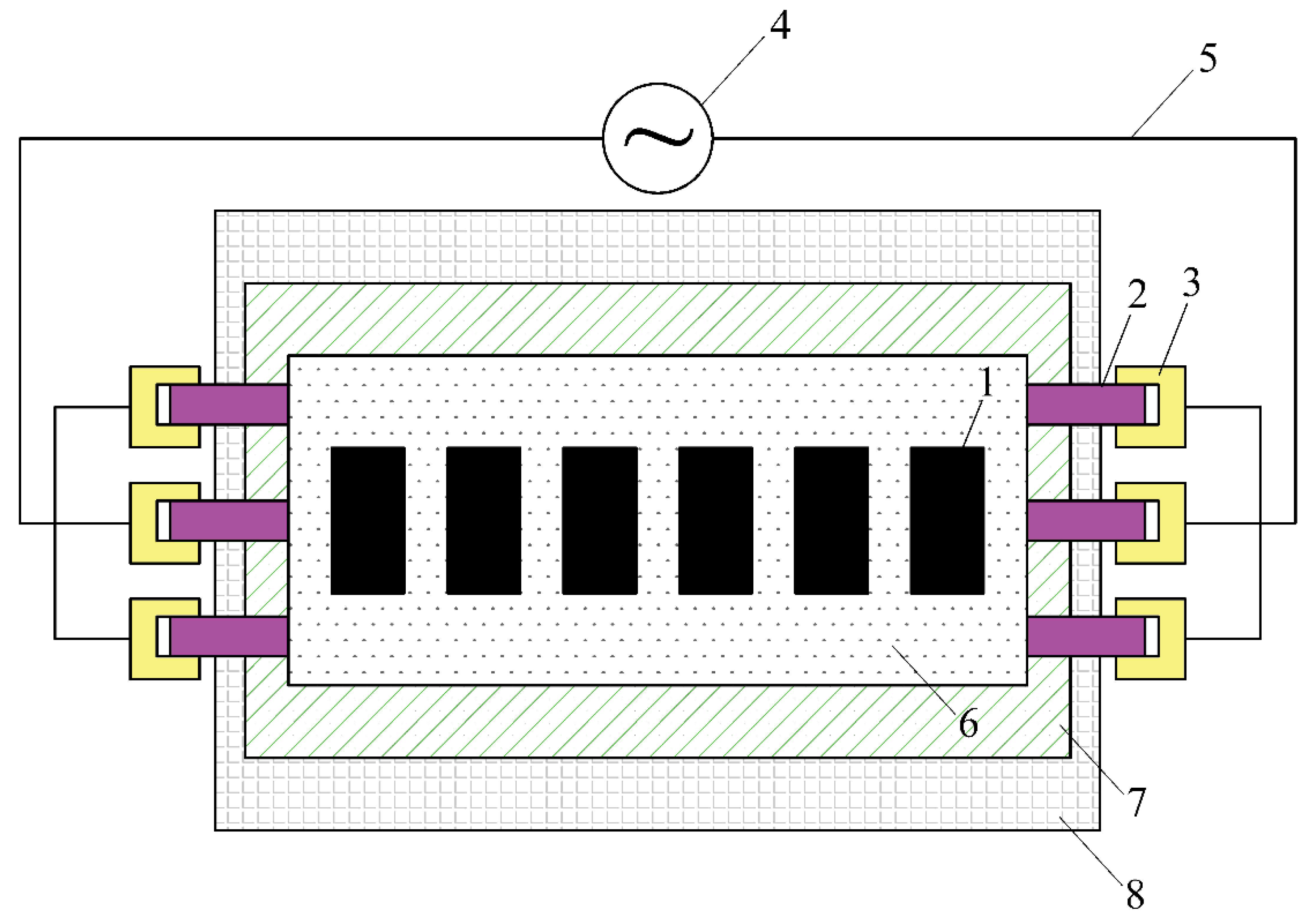
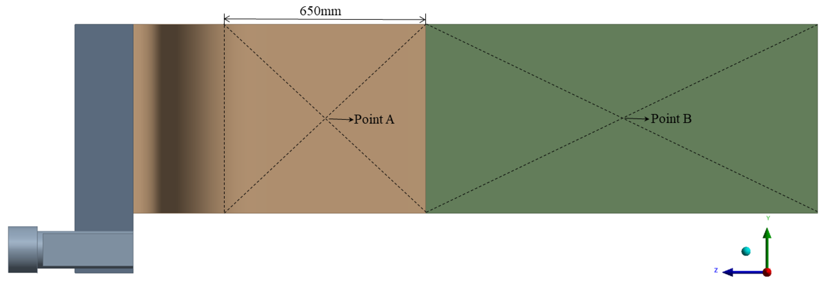
2.1. Research Subject

The power transmission clamp investigated in this paper is utilized in an Acheson graphitization furnace (AGF), specifically designed for the production of anode materials for lithium-ion batteries. Figure 1 depicts a schematic diagram of its structure. Within the furnace body, the carbon material is enclosed by resistive material, which in turn is surrounded by insulating material. During the graphitization process, electricity is supplied to the electrode array at the furnace head through conductors and the power transmission clamp. This array then conveys the current into the internal resistive material, generating ohmic heat to bake the carbon material. Similarly, the current flows back to the power source via the electrode array at the furnace tail, traversing through the power transmission clamp and conductors, completing the circuit.

In AGFs, the power transmission clamp performs two pivotal roles: conducting electric current and mechanically securing the electrodes. The quality of its design is crucial to the energy efficiency and operational stability of the graphitization process. Figure 2 illustrates the three-dimensional design of the power transmission clamp, comprising three main components: the connector (a), the cold plate (b), and the splint plate (c). The connector interfaces with liquid-cooled conductors; the splint plate secures the electrode blocks and forms the electric pathway. And the cold plate bridges the connector and splint plate, utilizing internal liquid-cooled channels to regulate temperature, ensuring the entire assembly operates within safe limits and prevents overheating.

To further elucidate the functioning of the power transmission clamp, Figure 2 also includes a depiction of the electrode block (d) protruding from the furnace. This section of the electrode block measures 1350 mm in length, 680 mm in width, and 650 mm in height. One end of the block is clamped by the power transmission clamp, while the other end extends into the resistive material inside the furnace. Together, the electrode block and power transmission clamp constitute the power delivery module of the AGF.

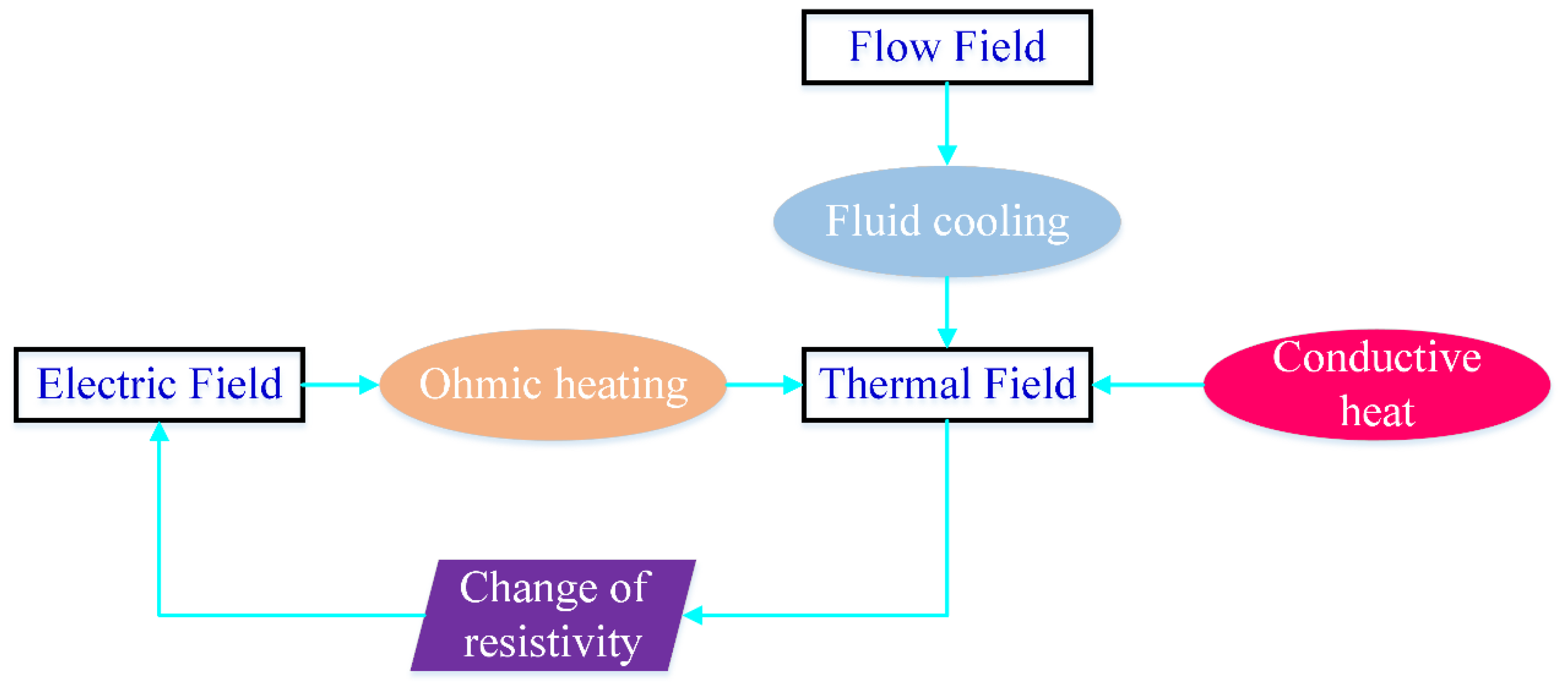
2.2. Electric-Thermal-Fluid Coupling Process

Generally, it is desirable for power transmission clamps to exhibit as little potential difference as possible to conserve energy consumption. Simultaneously, the clamp must be maintained within an appropriate temperature range. By this means, minimal temperature gradients can be obtained to prevent high-temperature burnout or thermal stress damage. To achieve this, a comprehensive and nuanced understanding of the clamp from the perspective of electric, thermal, and fluid field coupling is essential.

As illustrated in Figure 3, the electric, thermal, and fluid field coupling mechanisms during the operation of the power delivery module, comprising the power transmission clamp and electrode block, are presented.

Firstly, the electric current flows through the clamp and electrode block, generating ohmic heat, which serves as the internal heat source determining the temperature distribution. Secondly, due to the extreme temperatures within the AGF and the high thermal conductivity of the electrode material, a portion of this heat is transferred to the clamp through the electrode block via thermal conduction. Thirdly, to maintain a reasonable temperature distribution on the clamp, cooling fluid flows within the channels of the cold plate, forming a flow path and providing cooling to the clamp through wall heat exchange. Lastly, since the resistivity of the materials comprising both the clamp and electrode block varies with temperature, the temperature distribution in the thermal field reciprocally influences the electric field.

2.3. Mathematical Model

Based on the aforementioned description of the coupling processes, three-dimensional transient governing equations are formulated for the electric, fluid, and thermal fields, respectively.

(1)

Electric Field Governing Equation

The transient electric field is governed by the following equations:

$$\nabla \cdot \mathit{J}=Q_j$$

(1)

$$\mathit{J}=\sigma \mathit{E}$$

(2)

$$\mathit{E}=-\nabla \phi$$

(3)

where J is the current density, A/m³; Q_j is the current source, A/m³; σ is the electrical conductivity of the material, S/m; E is the electric field intensity, V/m; φ is the electric potential, V; ∇ denotes the vector differential operator.

For these equations, Equation (1) is the current conservation equation, indicating that the vector flux of current density in any closed region is equal to the current source in the region. Equation (2) is the differential form of Ohm’s law, indicating that the current density J is proportional to the electric field intensity E, and the proportional coefficient is conductivity σ. Equation (3) describes the relationship between electric field strength and potential; that is, the electric field strength points to the direction where the potential decreases fastest.

(2)

Fluid Field Governing Equation

The fluid motion in the transient fluid field is governed by the continuity equation and the momentum conservation equation [32]:

$$\nabla \cdot \mathit{V}=0$$

(4)

$$\nabla \cdot ({\rho }_l\mathit{V}\mathit{V})=-\nabla p+\nabla \cdot [\mu (\nabla \mathit{V}+{(\nabla \mathit{V})}^T)]+{\rho }_l\mathit{g}$$

(5)

where V is the velocity vector, m/s; ρ_l is the fluid density, kg/m³; p is the pressure, Pa; μ is the dynamic viscosity of the fluid, Pa·s; g is the gravitational acceleration, with its value to be 9.81 m/s².

The left side of Equation (5) represents the rate of change of fluid microelement momentum, and the right side includes pressure gradient, viscous force (determined by the dynamic viscosity μ of the fluid), and gravity, which jointly determine the motion of the fluid.

(3)

Thermal Field Governing Equation

The thermal field is governed by the heat conduction differential equation:

$${\displaystyle \frac{\partial (\rho cT)}{\partial t}}=\nabla (\lambda \nabla T)+S_{\phi }$$

(6)

where ρ is the density of the fluid or solid material in the computational domain, kg/m³; c is the specific heat capacity, J/(kg·K); T is the temperature, K; t is time, s; λ is the thermal conductivity of the fluid or solid material in the computational domain, W/(m·K); S_φ is the heat source term, W/m³.

The left side of Equation (6) represents the rate of change of heat per unit volume with time, and the right side includes the effect of heat conduction (determined by thermal conductivity λ) and heat source S_φ on the temperature field.

Heat exchange between the fluid and solid domains occurs through convection:

$$q=h\Delta T$$

(7)

where q is the heat flux density on the solid wall in contact with the fluid, W/m²; h is the convection heat transfer coefficient related to flow velocity and pattern, W/(m²·K); ΔT is the temperature difference between the fluid and solid wall, K.

In this study, the heat source term S_φ represents the Joule heat generated by the electric current flowing through solid materials, thereby coupling the electric and thermal fields:

$$S_{\phi }=\mathit{J}\cdot \mathit{E}$$

(8)

Joule heat is an important coupling mechanism between electric field and thermal field. The dot product of current density J and electric field intensity E represents Joule heat generated in unit volume, which will affect the temperature distribution of materials.

Furthermore, the electrical conductivity σ of various materials in the electric field solution varies with the local temperature T, necessitating the incorporation of thermal field results into the electric field solution process:

$$\sigma =\sigma (T)$$

(9)

3. Numerical Simulation and Validation

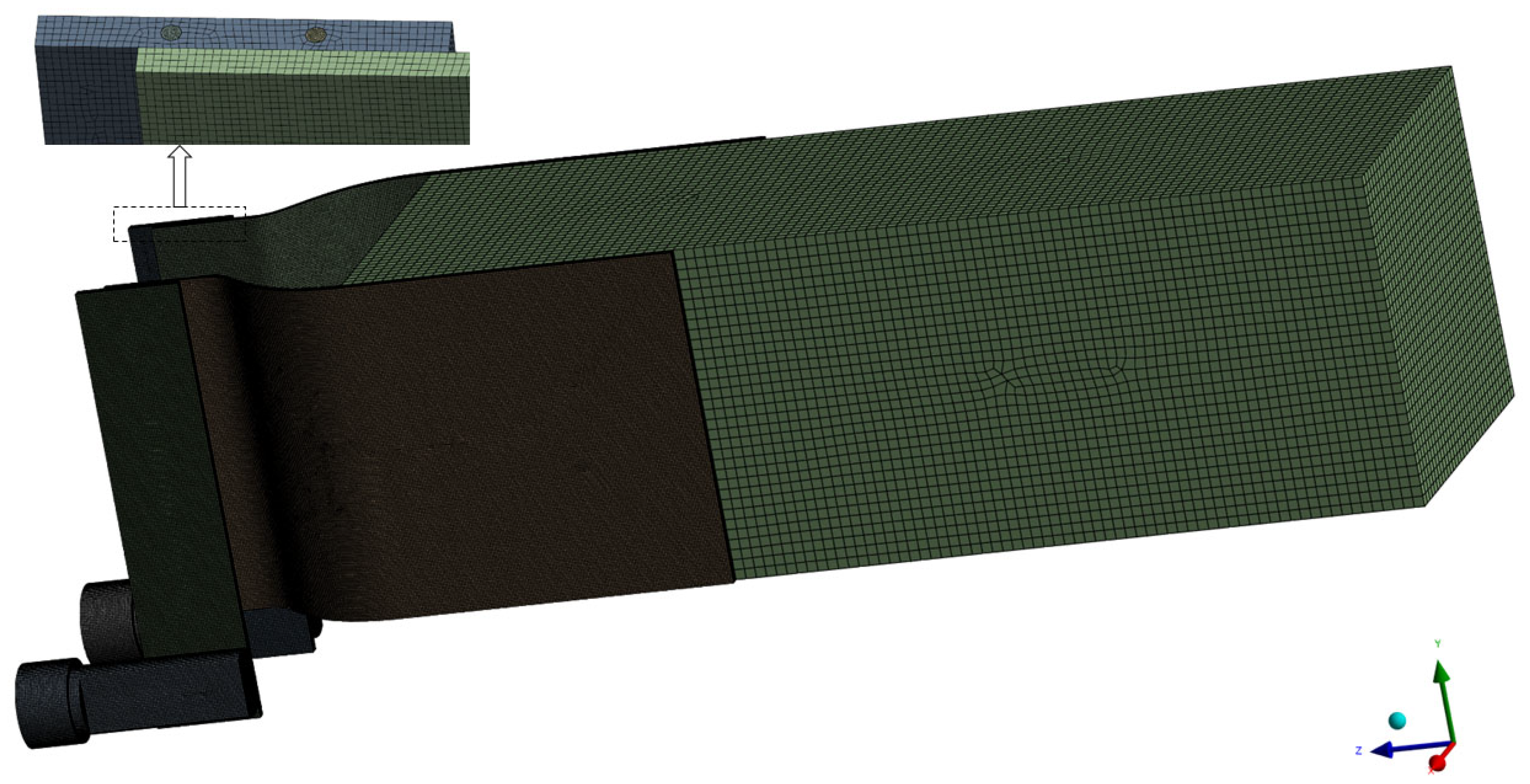
3.1. Mesh and Material Properties

The entire process of establishing and solving the numerical model, encompassing three-dimensional model creation, meshing, model setup, solution, and post-processing, was conducted on the commercial software platform ANSYS Workbench 2023R1. The geometry module was utilized for three-dimensional model construction, while the Meshing module facilitated grid generation. The resulting hexahedral mesh is illustrated in Figure 4, and the statistics on the number of elements, nodes, and mesh quality are summarized in

Table 1. Mesh statistics.

Node Number	Element Number	Element Quality		Skewness		Orthogonal Quality
		Average	Standard Deviation	Average	Standard Deviation	Average	Standard Deviation
1,529,537	1,546,593	0.877	0.186	0.209	0.082	0.934	0.191

. As evident from Table 1, the average element quality and orthogonal quality are impressively high at 0.877 and 0.934, respectively, with both standard deviations remaining below 0.2, indicating an overall high-quality mesh.

In the model, the power transmission clamp, comprising the connector, cold plate, and clamping plate, is made of copper alloy, while the electrode block is composed of graphite. The material properties of these two solid materials are listed in

Table 2. Solid material properties.

Material		Copper Alloy	Graphite
Density (kg·m−3)		8933	2300
Specific heat capacity (J·kg−1·K−1)		385	710
Thermal conductivity	Reference value (W·m−1·K−1)	390	680
	Temperature coefficient (K−1)	−2.02 × 10−4	6.12 × 10−4
Electric conductivity	Reference value (S·m−1)	5.96 × 107	7.53 × 105
	Temperature coefficient (K−1)	−8.10 × 10−4	6.12 × 10−4

[33,34]. Notably, the thermal conductivity and electrical conductivity of these materials vary approximately linearly with temperature, as described by the following equation:

$$L(T)=L_0[1+\alpha (T-T_0)]$$

(10)

where L(T) represents the thermal conductivity (or electrical conductivity) at temperature T; T₀ is the reference temperature, set at 20 °C in this study; L₀ is the thermal conductivity (or electrical conductivity) at the reference temperature; and α is the temperature coefficient.

3.2. Model Setup and Solving

The model setup and solution process were carried out within the CFX 2023 software module, which employs a finite volume method based on finite elements. This approach combines the conservation properties of the finite volume method with the numerical accuracy of the finite element method [35]. Model configuration primarily encompasses the specification of initial conditions, boundary conditions, and contact conditions.

3.2.1. Initial Conditions

At the commencement of a working cycle, the AGF remains unpowered, the coolant circulation pump remains idle, and the temperature throughout is uniformly aligned with the ambient surroundings. Based on this, the initial conditions are defined as follows:

(1)

Ambient temperature: The entire computational domain is initialized at an ambient temperature of 20 °C.

(2)

Fluid flow: The fluid domain is initialized with a velocity of 0 m/s and a gauge pressure of 0 Pa.

(3)

Electric potential: The entire solid domain is initialized with an electrical potential of 0 V.

3.2.2. Boundary Conditions

Boundary conditions encompass thermal, fluid flow, and electrical types:

(1)

Thermal boundary conditions

As depicted in Figure 5, the end face of the electrode block farthest from the power transmission clamp is assigned a time-varying temperature profile, derived from actual measurements taken by thermocouples during the AGF operation process at the interface between the electrode and the AGF’s outer wall. The standard length of the AGF production cycle in this study is 48 h. For convenience of expression, the abscissa in the figure uses hour (h) as the unit of time measurement. The end face of the connector, in contact with an externally cooled liquid cable, maintains a nearly constant temperature due to effective cooling by the coolant. Therefore, the connector’s end face temperature is set to the average cable temperature of 40 °C. For other exterior surfaces in the model, exposed to the air, convective heat transfer boundary conditions are applied, with a heat transfer coefficient of 10 W/(m²·K) and an ambient temperature of 40 °C.

(2)

Fluid Flow Boundary Conditions

The liquid-cooled channels are filled with deionized water. According to the actual operational parameters, the top and bottom of the liquid-cooled channels in Figure 2 are designated as inlet and outlet boundary conditions, respectively. Specifically, the inlet boundary condition is set with a normal velocity of 0.5 m/s and a temperature of 25 °C. The outlet boundary condition is defined by setting the average gauge pressure at the outlet to 0 Pa.

(3)

Electrical Boundary Conditions

The end face of the electrode block farthest from the power transmission clamp is designated as the zero-potential surface. Meanwhile, a time-varying total current is applied to the end face of the connector, as illustrated in Figure 5. The horizontal axis in Figure 5 represents the operating time, with the left vertical axis indicating the total current value and the right vertical axis showing the temperature of the electrode block’s end face distant from the clamp. The time-varying curves of total current and temperature in Figure 5 are derived from actual measurements taken during a production cycle in an industrial setting, spanning a total duration of 48 h.

3.2.3. Contact Conditions

The physical components of this model comprise the connector, cold plate, splint plate, liquid-cooled channels, and electrode block. Contact conditions are established between the interfaces of these components. Specifically, thermal and electric contacts involve the connector-cold plate, cold plate-splint plate, and splint plate-electrode block contact pairs, while the cold plate-liquid-cooled channel contact pair only includes thermal contact. In this study, a simplifying assumption is made that the contact electric resistance and contact thermal resistance between all contact pairs are negligible, approximating them to zero.

3.2.4. Solving Setup

Given that a complete operating cycle of the AGF lasts 48 h, the total calculation duration is set accordingly. The calculation process employs an equal time step strategy, with each step lasting 5 min, resulting in a total of 576 time steps. The advection and transient schemes are configured as high resolution and second-order backflow Euler, respectively, and the residual target in the convergence control is set below 10⁻⁴ (RMS). To achieve sufficiently high solution accuracy, the double precision separation implicit algorithm is employed.

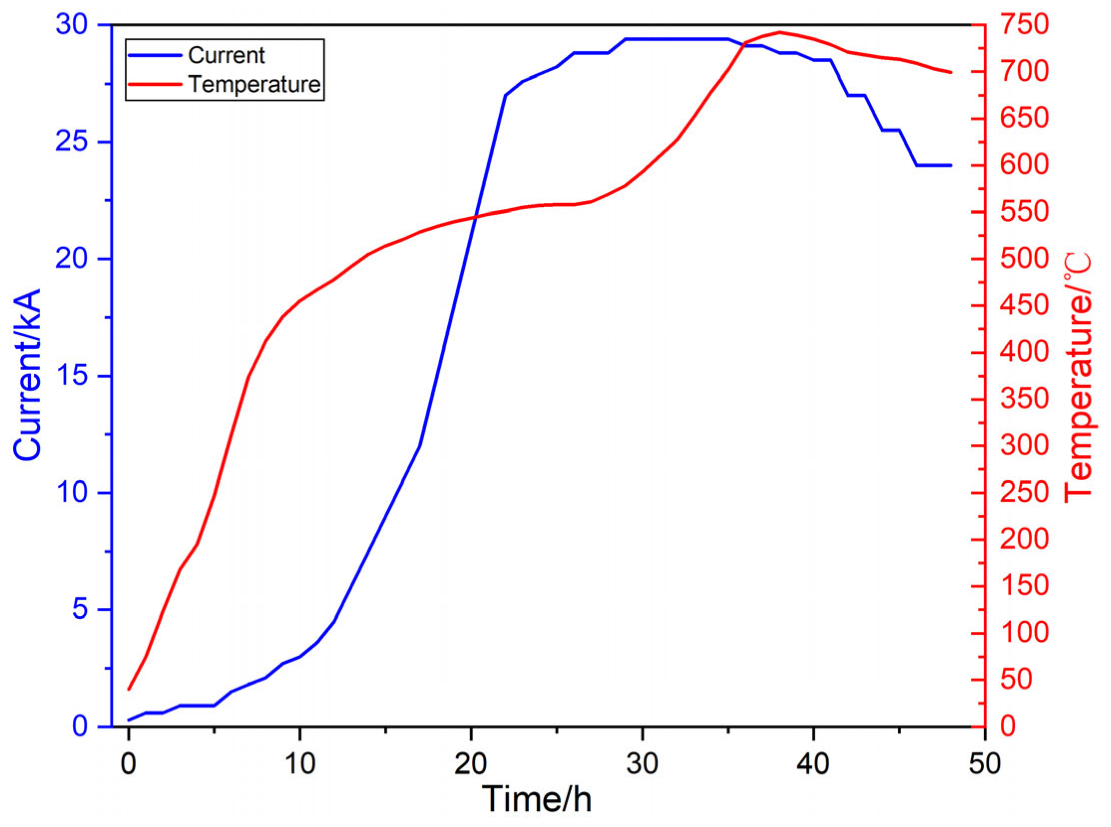
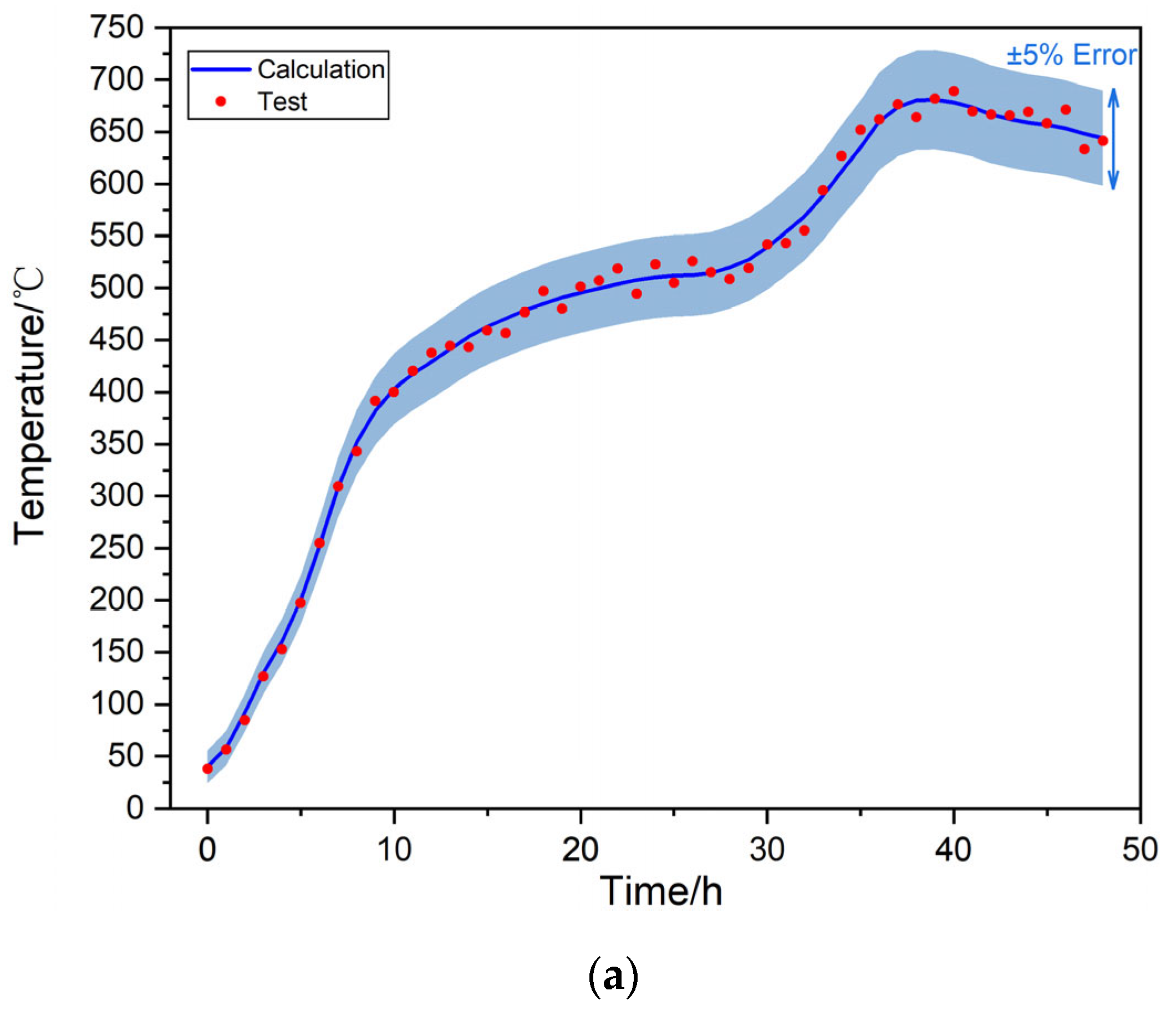
3.3. Test Validation

To validate the numerical results, two monitoring points, Point A on the splint plate and Point B on the electrode block, are selected for comparison between experimental data and simulation results. The locations of these monitoring points are depicted in Figure 6. These two monitoring points are located at the rectangular centroid of the flat surface of the splint plate and electric block to facilitate the positioning during testing. During a complete operating cycle, temperature measurements are taken at both monitoring points every hour using a nickel–chromium–nickel–silicon thermocouple. Its measurement range is 0 to 900 °C, and its accuracy is ±2.5 °C.

The comparison between the measured and calculated temperatures at Points A and B is presented in Figure 7a and Figure 7b, respectively. The calculated value is derived from the information extraction of the corresponding coordinate points in the calculation result file. And the color bands in Figure 7 represent the ±5% temperature range around the calculated values at each time point. Figure 7 demonstrates good agreement between the calculated and measured values, with deviations controlled within 5%, confirming the high reliability of the model’s predictions in this study.

4. Results and Discussion

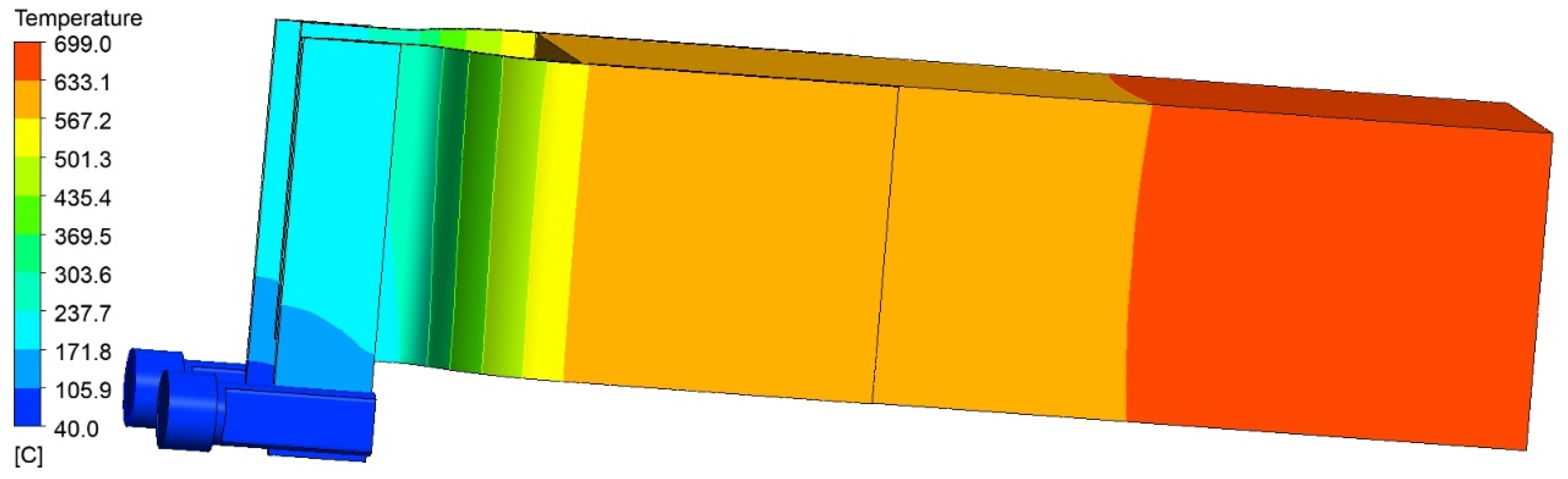
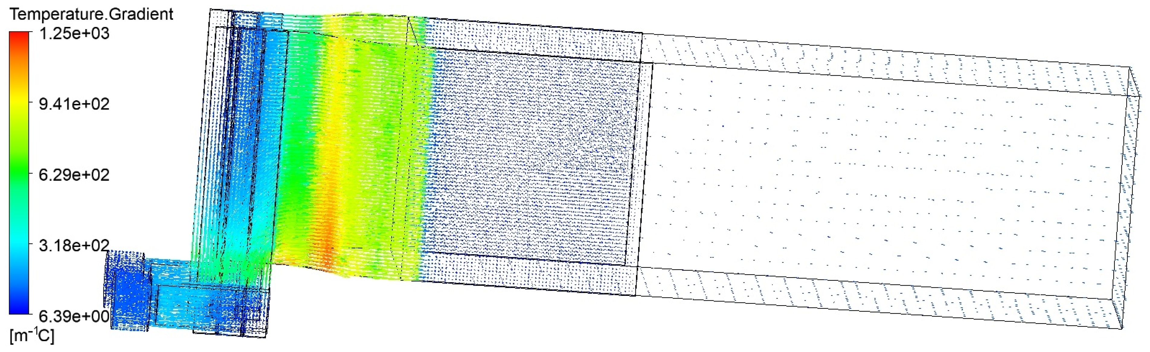
4.1. End-Time Distribution

Taking the end of a working cycle as an example, Figure 8 and Figure 9 present the temperature and potential distribution contours of the studied components, respectively. As the temperature of AGF is increasing during the working process, the end time of a working cycle is selected to observe the temperature and potential distribution characteristics. As seen in Figure 8, significant temperature differences exist across the power transmission module. Specifically, the end face of the electrode block nearest the furnace core attains the highest temperature of 699 °C, while the lowest temperature of 40 °C is recorded at the end face of the connector. The graphite material composing the electrode block, with its high thermal conductivity and large cross-sectional area in a rectangular shape, exhibits relatively small temperature differences. In contrast, the power transmission clamp exhibits more pronounced temperature variations. This is because it has complex geometry and various cooling mechanisms, which include thermal conduction at the connector, convective heat transfers at the liquid-cooled channel walls, and natural convection at the exterior surfaces.

Figure 9 reveals that at the conclusion of the graphitization process, the total potential difference across the power transmission assembly is approximately 120 mV. The potential decreases from the connector end face to the electrode block end face adjacent to the furnace core.

Furthermore, the temperature gradient and current density distributions within the power transmission module are depicted in Figure 10 and Figure 11, respectively, in vector form. The temperature gradient indicates the direction and rate of maximum temperature change within the studied region, typically pointing towards regions of increasing temperature. Figure 10 highlights significant temperature gradients at the bends of the clamping plate, suggesting substantial material expansion differences in these areas, leading to considerable thermal stress and potential failure risks. Notably, the temperature gradient at the bends is not uniform but exhibits an increasing trend from top to bottom, influenced not only by specific heat transfer relationships but also to a certain extent by the electric field distribution. As illustrated in Figure 11, current initially flows into the lower connector, then diagonally upwards through the thin liquid-cooled plate and splint plate before entering the electrode block, resulting in higher current densities and consequently greater ohmic heating below the bends of the splint plate compared to above.

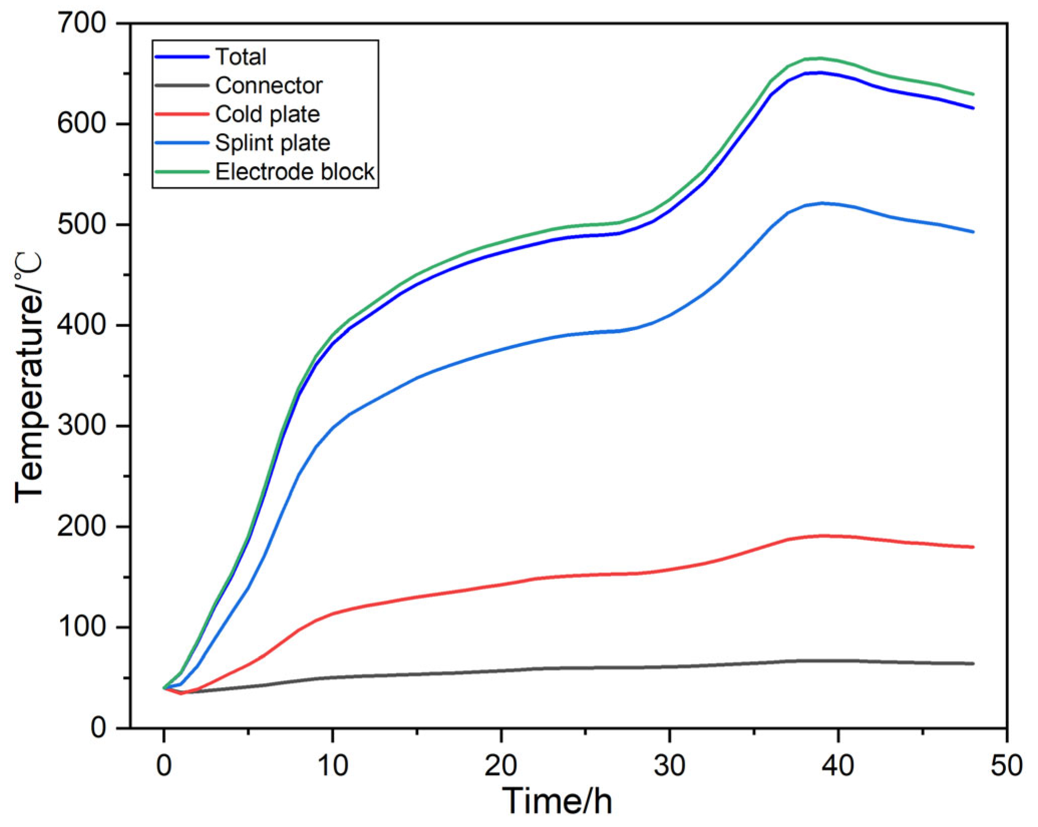
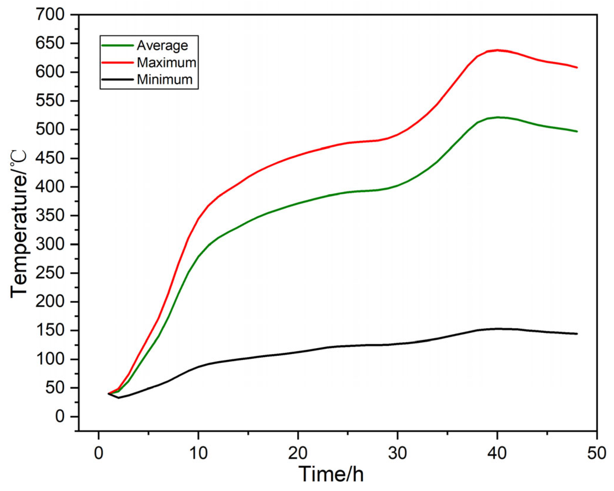
4.2. Temporal Variation of Temperature

To comprehend the temperature evolution throughout the graphitization process, the overall average temperature of the module and the average temperatures of individual components at each time step were analyzed, resulting in the temporal curves presented in Figure 12. The average temperature of a component is calculated by integrating its temperatures over volume and dividing by the total volume, encompassing the connector, cold plate, splint plate, and electrode block. The overall average temperature represents the mean temperature across the entire computational model. As seen in Figure 12, the electrode block exhibits the highest average temperature during graphitization, contributing significantly to the overall average temperature due to its 95% volume share within the model. For the power transmission clamp, the connector and cold plate maintain low average temperatures owing to effective cooling. And the splint plate, in direct contact with a large area of the electrode block, follows a similar temperature trend with a maximum value exceeding 500 °C.

During the initial and intermediate stages of Figure 12, the average temperatures of all components rise with graphitization but exhibit a declining trend towards the end, correlated with the total current and electrode block end-face temperature shown in Figure 5. The Pearson product-moment correlation coefficient (PPMCC) was employed to quantitatively assess these relationships. The PPMCC, ranging from −1 to 1, measures the correlation between two variables. High positive values (close to 1) indicate strong positive correlations, while high negative values (close to −1) indicate strong negative correlations.

Table 3. PPMCC between different parameters.

Average Temperature	Total Current	End-Face Temperature of Electrode Block
Total	0.848	0.999
Connector	0.914	0.978
Cold plate	0.883	0.991
Splint plate	0.856	0.996
Electrode block	0.847	0.999

lists the PPMCC values between the average temperatures of various components and the total current, as well as the electrode block end-face temperature. Notably, the PPMCC values between the electrode block end-face temperature and the average temperatures of all components are consistently above 0.99, significantly higher than those between the total current and average temperatures. This suggests that thermal conduction from the high-temperature end face of the electrode block predominantly influences temperature variations within components, with ohmic heating due to current having a relatively minor impact.

In practice, the temperature variation characteristics of the electrode clamp, particularly the maximum temperatures and temperature differences among components, are of great concern to prevent burnout or thermal stress damage. Figure 13 summarizes the maximum, minimum, and average temperatures of the power transmission clamp at each time step, revealing a pronounced increase in temperature differences during graphitization. The peak value of maximum temperature is 640 °C, which is obtained at t = 39 h. The average temperature follows a similar trend to the maximum, while the minimum temperature exhibits a more gradual increase.

Further, Figure 14 plots the differences between the maximum and minimum temperatures of individual components within the power transmission clamp at various time points during graphitization. Notably, the splint plate consistently experiences the highest temperature differences, with a maximum value approaching 500 °C. The cold plate and electrode block exhibit moderate temperature differences, controllable within 150 °C, while the connector maintains the lowest differences, within 50 °C. Thus, during graphitization, the splint plate, with its significant temperature differences and high maximum values, poses the greatest risk of thermal degradation and requires close attention. This is attributed to its elongated and flat shape, long thermal conduction paths, and partial contact with the cold plate versus extensive contact with the high-temperature electrode block, leading to substantial temperature variations influenced by its geometry and surrounding heat transfer conditions.

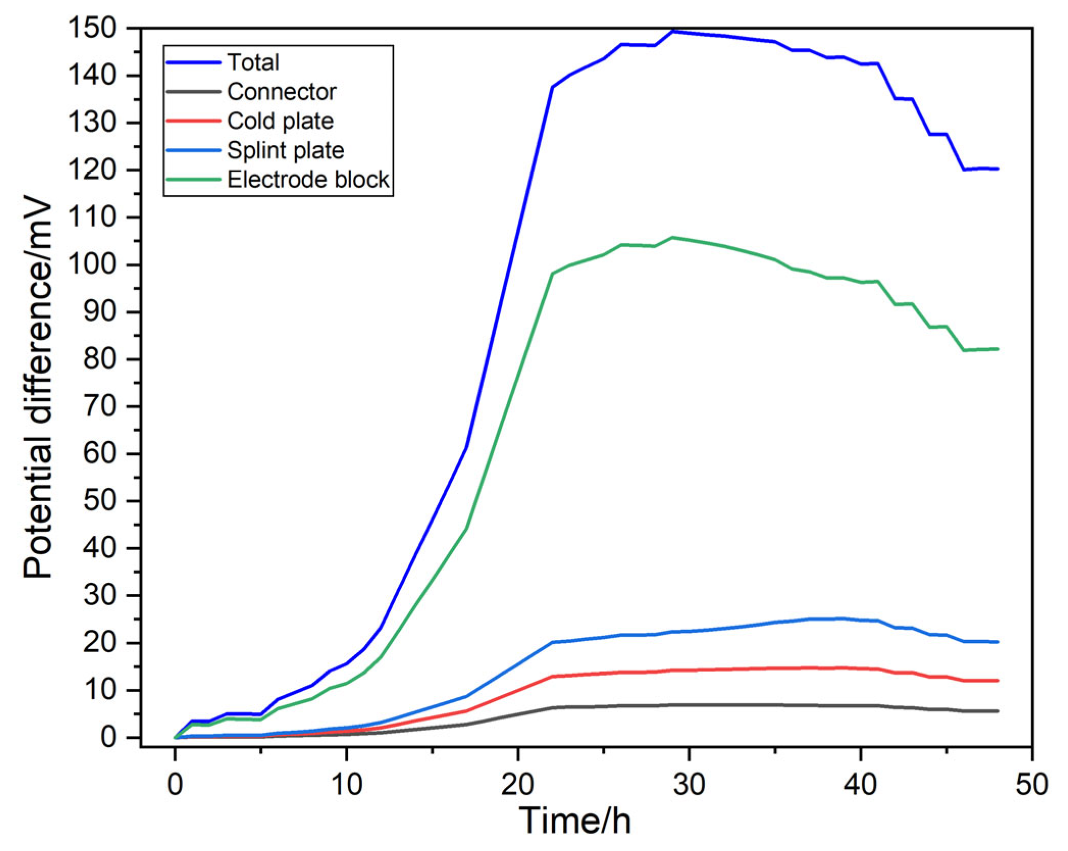
4.3. Temporal Variation of Potential Differences

Apart from thermal conditions, potential differences that are directly related to the power consumption of the AGFs are also a focal point of this study. Figure 15 depicts the temporal variations of potential differences across various components during the graphitization process, along with the total potential difference across the power transmission assembly. According to Ohm’s law, the potential difference across a conductor is the product of the current flowing through it and its resistance. Consequently, the temporal patterns of the potential difference curves align with the current variations shown in Figure 5. Notably, the electrode block contributes the largest proportion to the total potential difference, followed by the splint plate, while the cold plate and connector exhibit lower potential differences.

Dividing the potential differences by the respective current values at each time step reveals the temporal variation of resistance for different components, as shown in Figure 16. This figure indicates that the resistance of the electrode block generally decreases as the graphitization process progresses. Since the electrode block accounts for a significant portion of the total potential difference across the power transmission module, the overall resistance of the module also exhibits a moderate decreasing trend. In contrast, the resistance of the splint plate increases overall. These phenomena stem from the different temperature coefficients of electrical conductivity between the graphite material comprising the electrode block and the copper alloy of the transmission clamp. As listed in Table 2, the temperature coefficients of electrical conductivity for graphite and copper alloy are 6.12 × 10⁻⁴ K⁻¹ and −8.10 × 10⁻⁴ K⁻¹, respectively. Therefore, as temperatures rise during graphitization, the electric conductivity of graphite increases, while that of copper alloy decreases, leading to opposite trends in resistance changes between the electrode block and splint plate.

By dividing the power transmission module into the electrode block and power transmission clamp, the temporal variation of their respective resistance proportions over a working cycle is summarized in Figure 17. The figure reveals that the electrode block’s resistance initially accounts for 79% of the total resistance but decreases to 67.5% at t = 39 h, a decline of approximately 11.5 percentage points. This analysis underscores that the electrode block’s dominance in the total resistance, combined with graphite’s decreasing resistivity with rising temperatures, favors a reduction in the module’s power consumption as AGF operating temperatures increase.

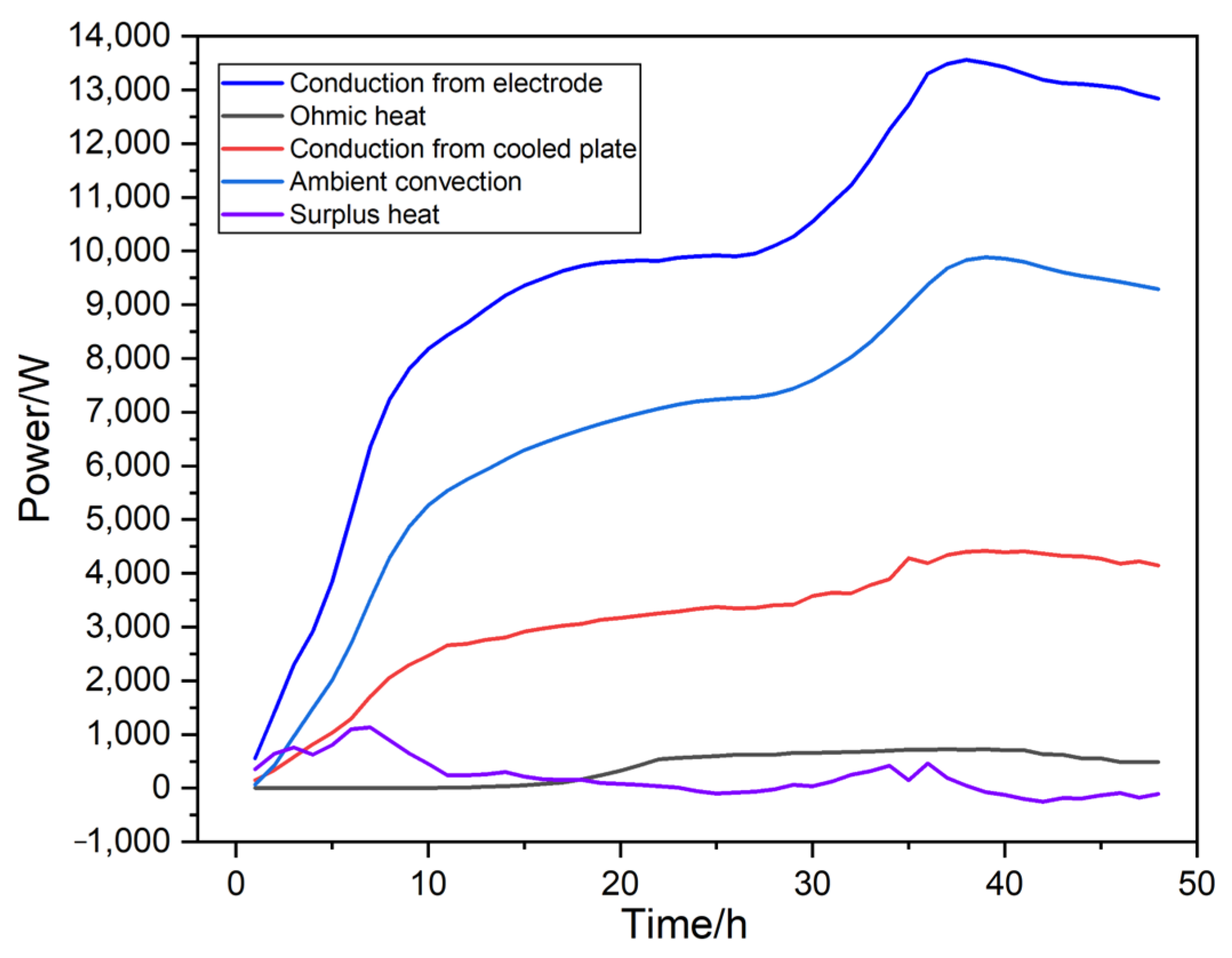
4.4. Heat Budget Analysis

To understand the factors governing temperature and resistance variations across components and provide targeted guidance for temperature difference control and potential difference reduction in the power transmission clamp, an in-depth analysis of the heat budget within the power transmission module is necessary.

Figure 18 and Figure 19 present the temporal variations in heat income and expenditure for the entire computational model during the graphitization process, respectively.

As shown in Figure 18, heat income primarily comprises thermal conduction and ohmic heating, with thermal conduction contributing far more power than ohmic heating. The thermal conduction heat source originates from the AGF core, which operates at extremely high temperatures (up to 3000 °C). The graphite electrodes between the core and power transmission clamp act as efficient thermal conductors, ensuring that heat transfer from the core to the module dominates the heat income.

Further observation reveals two peaks in the thermal conduction power at t = 7 h and t = 36 h, marking the transitions between three distinct production stages. From the initial graphitization stage to t = 7 h, the preheating stage gradually increases heating power to elevate material temperatures and remove residual moisture. The period from t = 7 h to t = 36 h corresponds to the main process stage, where materials are baked and graphitized. During the early main stage, a relatively low temperature rise rate is maintained. This is to prevent cracking and facilitate stable carbon atom rearrangement from a disordered to an ordered structure, so a slightly lower thermal conduction power is set. In the later main stage, as carbon phase transitions intensify, graphite crystal structures mature, and graphitization rates accelerate, furnace temperatures rise, leading to a rapid increase in thermal conduction power to the power transmission module. In the final stage (t > 36 h), as graphitization nears completion, supply currents decrease, core temperatures drop, and the thermal conduction power to the module declines.

In contrast, heat expenditure occurs primarily through natural convection, thermal conduction via the connector end face with liquid-cooled cables, and liquid-cooled convection within the cooling channels. Figure 19 depicts the temporal variations of heat transfer power for these three mechanisms, along with the residual heat power, which is the difference between total heat income and expenditure. For the entire model, most heat is dissipated through natural convection with the ambient environment, while liquid-cooled convection and thermal conduction through the connector contribute negligibly. When t < 22 h, the residual heat power is positive, indicating an overall heating trend. Between t = 22 h and t = 38 h, residual heat power fluctuates around zero with modest absolute values, maintaining a net residual level and a moderate heating trend. When t > 38 h, residual heat power remains negative, signaling a gradual cooling of the power transmission module.

Given the splint plate’s high temperatures, largest temperature differences, and subsequent risk of thermal failure, a detailed heat budget analysis is conducted for this component, as shown in Figure 20. The splint plate’s heat income stems primarily from thermal conduction through the electrode and ohmic heating, while heat expenditure occurs via thermal conduction through the cold plate and natural convection with the environment. Figure 20 indicates that while thermal conduction through the electrode and natural convection dominate heat exchange, thermal conduction through the cold plate also contributes significantly to heat dissipation. The residual heat power for the splint plate, with t = 39 h as the dividing point, transitions from positive (heating trend) to negative (cooling trend), consistent with the average temperature variations shown in Figure 12.

Figure 21 further illustrates the heat budget of the cold plate, where most heat income originates from the splint plate and a minimal amount from ohmic heating. Heat expenditure comprises thermal conduction to the connector, liquid-cooled convection, and natural convection, with liquid-cooled convection consistently accounting for the highest proportion. Although natural convection with the ambient environment dominates heat loss for the entire model, forced convection within the cooling channels contributes most significantly to the cold plate’s heat dissipation and indirectly provides a crucial cooling pathway for the splint plate, which faces the highest risk of thermal failure. Therefore, well-designed cold plates and cooling channel structures, coupled with appropriate coolant flow rates and inlet temperatures, are crucial for the efficient and stable operation of the splint plate and the entire power transmission clamp.

4.5. Comparison with Previous Work

In prior AGF studies, researchers prioritized enhancing the furnace’s interior structure and material composition, along with its shell insulation structure, to optimize energy and electronic efficiencies. And the key analysis point was the numerical simulation of thermal-electric distribution within the furnace [19,23]. In contrast, our current work involves a comprehensive simulation of the transient electric-thermal-fluid coupling field within the power supply component. This simulation reveals that the operational power consumption, safety, and stability of the power delivery module in an AGF, consisting of the power transmission clamp and electrode block, are intimately tied to their mutually coupled electric-thermal distribution characteristics, which are further influenced by the coolant flow.

Our aim is to fill gaps in existing research and provide designers with a more comprehensive understanding of AGF’s thermal and electrical behaviors. Notably, we found that electrodes with high thermal conductivity are crucial for efficient heat dissipation from furnace materials. Moreover, maintaining an elevated electrode temperature is essential to reducing voltage drops. This underscores the importance of considering the impact of power supply components on overall power and heat distribution in AGFs for future research and development.

Meanwhile, the thermal behavior of the power delivery module studied herein is closely tied to the current and end-face temperature curves depicted in Figure 5. To further elucidate the trend of variations in its electric-thermal distribution, it is also imperative to undertake in-depth research by integrating it with the calculation model of the electric-thermal field within the furnace.

5. Conclusions and Future Work

5.1. Conclusions

This study developed and validated a 3D transient electric-thermal-fluid coupling model for the power delivery module of AGF using CFX to study its electrical and thermal distribution and variation characteristics during the working process. The insights from the analysis results aid in optimizing AGF power delivery module structure and process parameters for improved reliability and efficiency.

Some key findings are:

(1)

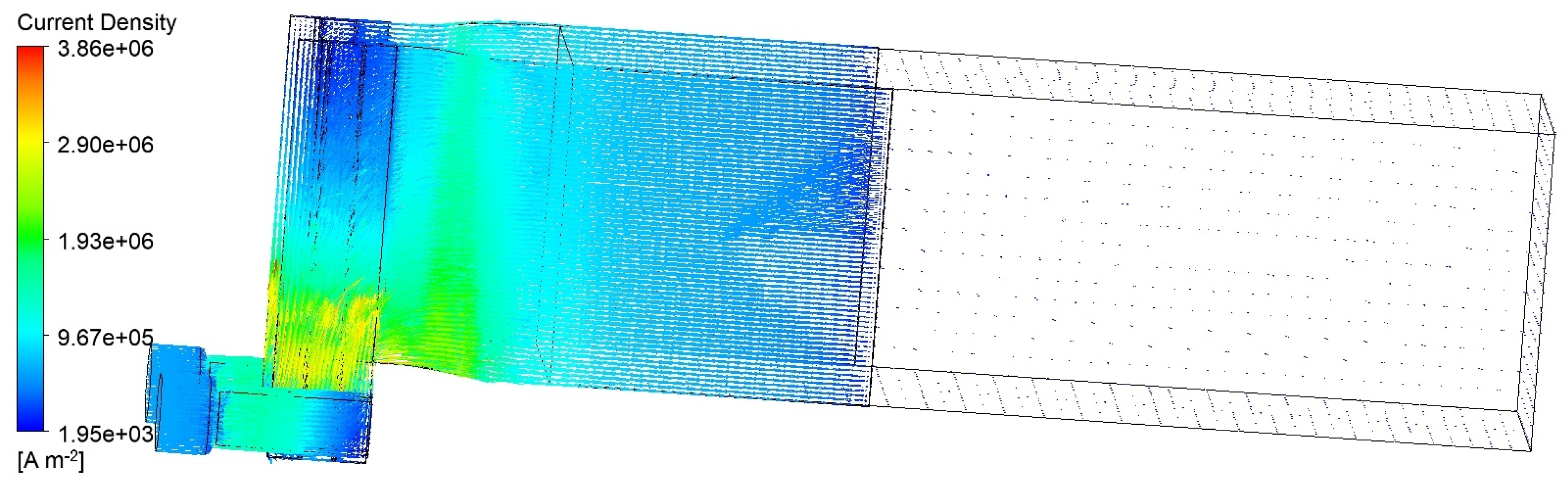
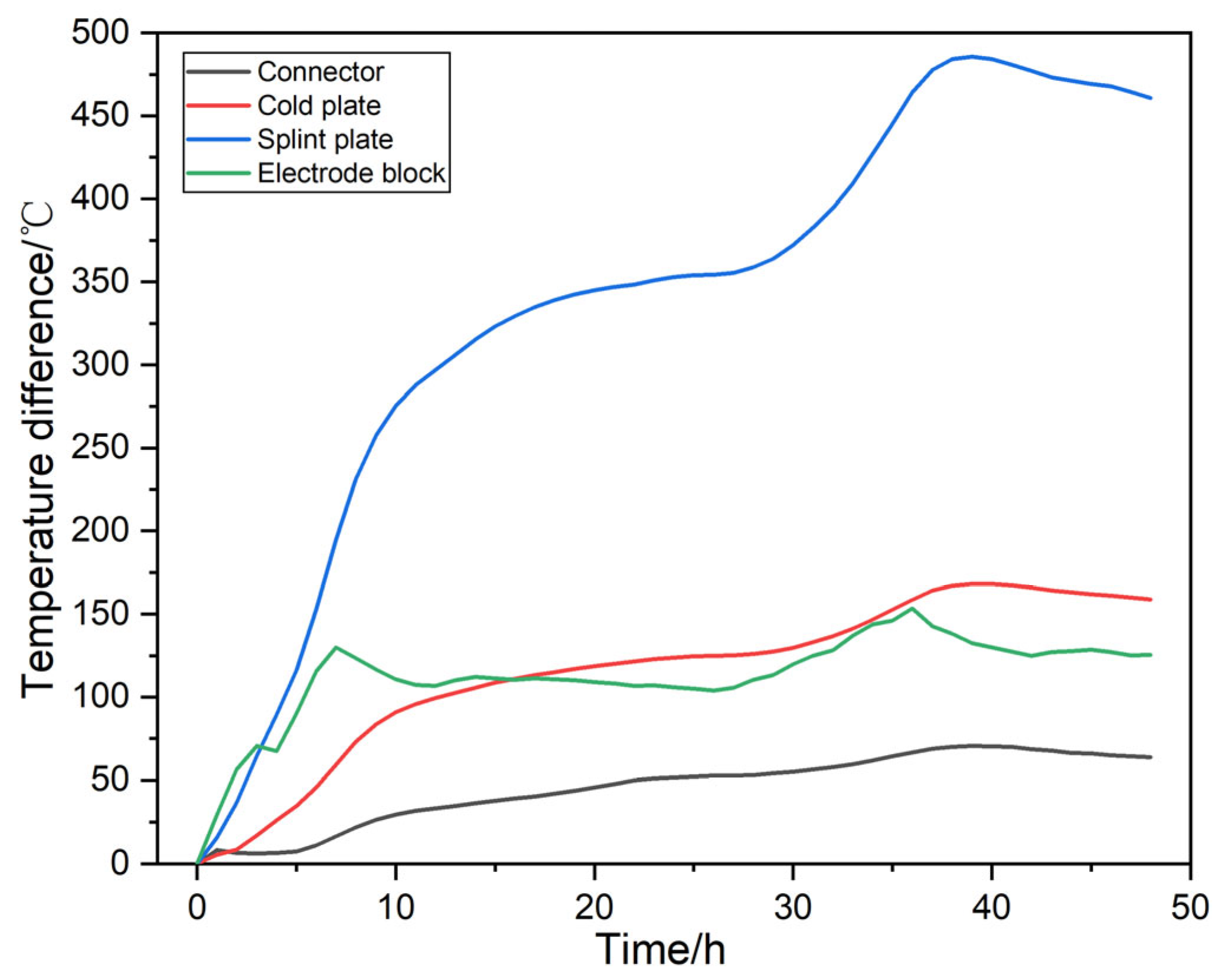
Significant temperature differences and potential failure risks: The power transmission module exhibits notable temperature differences, with the highest temperature observed at the electrode block end face proximal to the furnace core and the lowest at the connector end face. Temperature gradient and current density analyses reveal elevated thermal stresses and ohmic heating at the bends of the splint plate, posing potential failure risks. Additionally, the temperature differences within the splint during graphitization are also pronounced, necessitating close monitoring to prevent thermal damage.

(2)

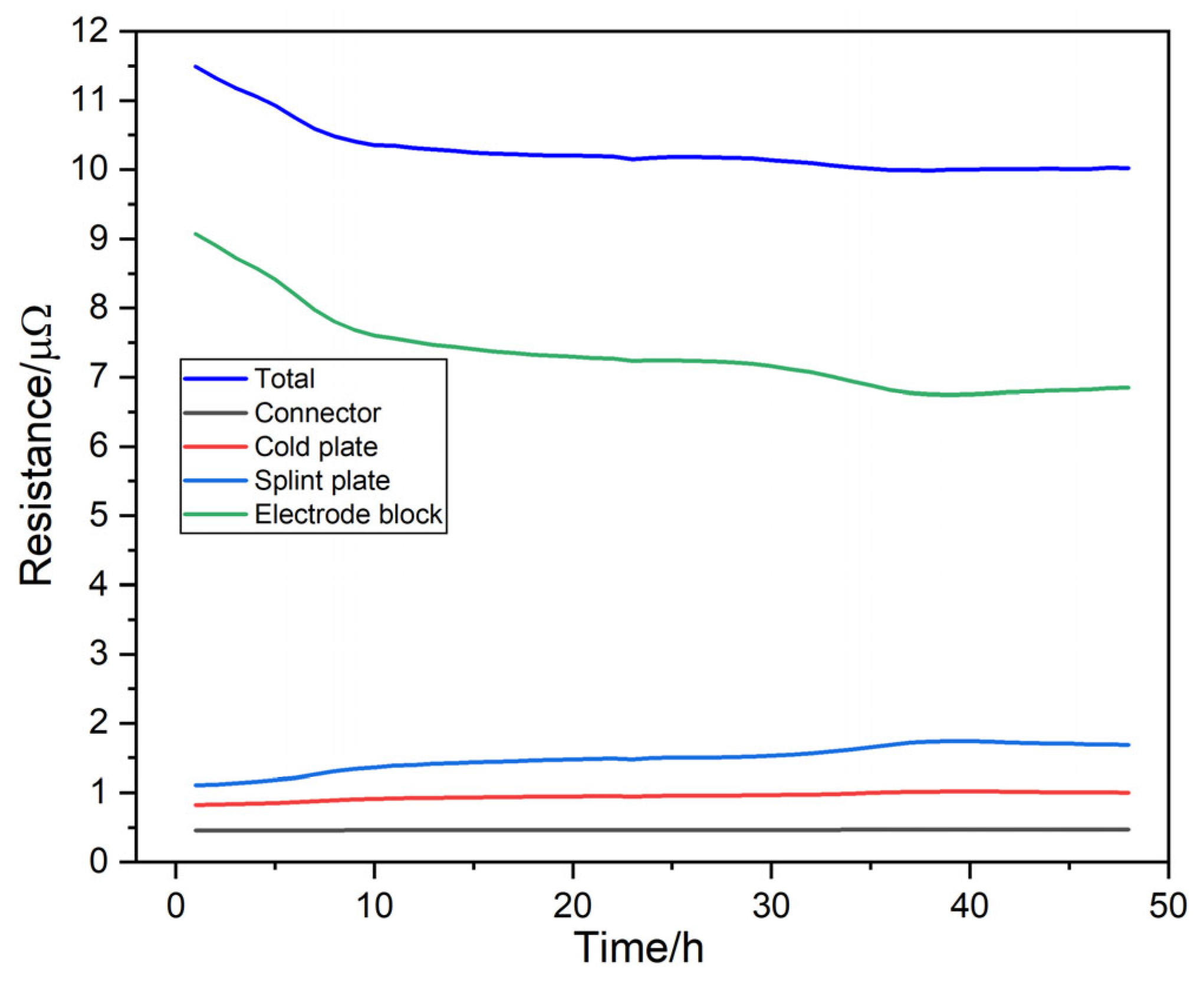
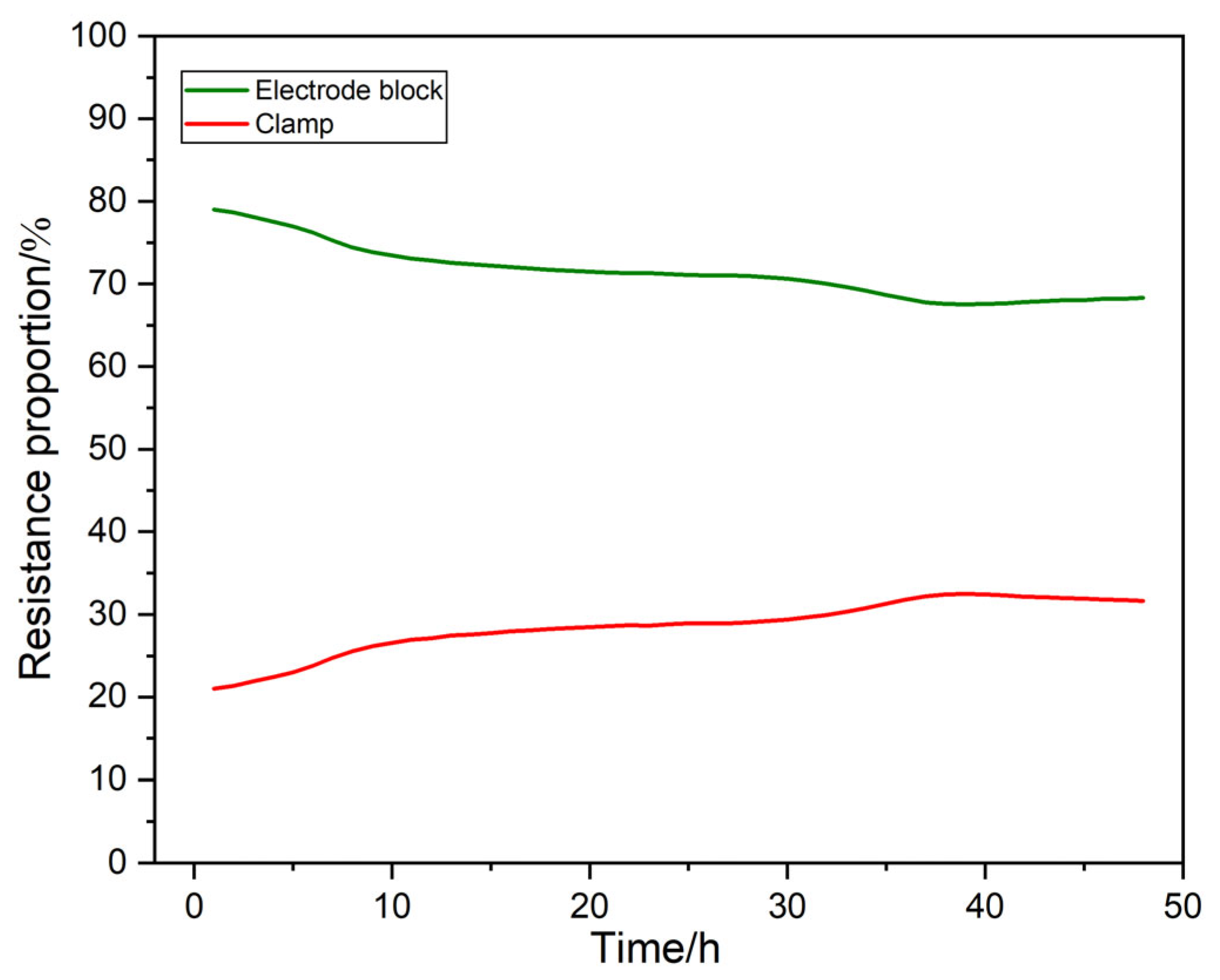
Resistance dominance and power savings: The electrode block accounts for a substantial portion of the total resistance within the power transmission module. Thus, maintaining relatively high temperatures, without compromising the splint plate, aids in keeping the total potential difference across the module at a relatively low level, thereby contributing to operational power savings.

(3)

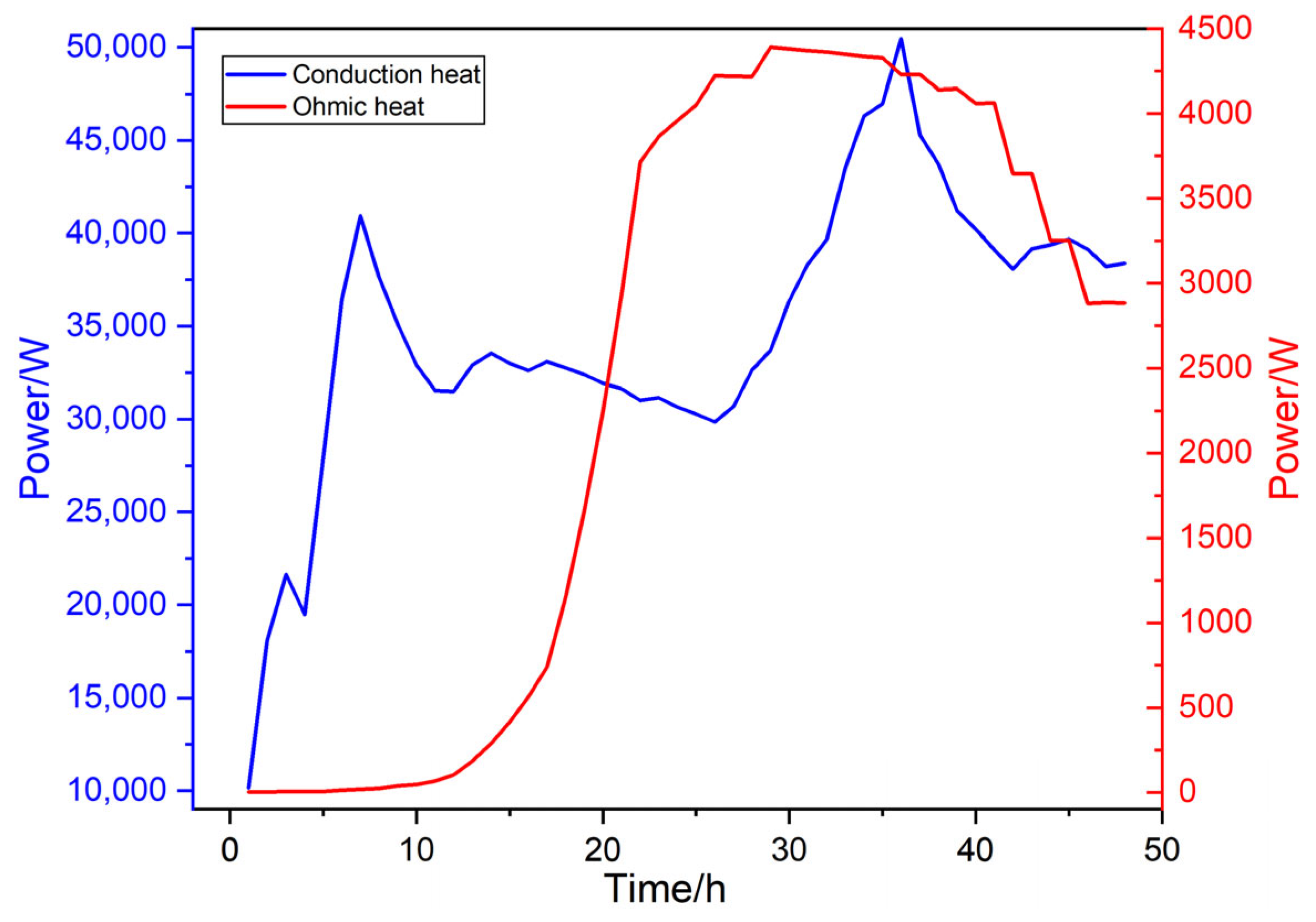
Heat budget analysis and efficiency enhancement: The primary heat source for the power transmission module is thermal conduction from the furnace core through the electrode. Natural convection and forced convection via liquid cooling are the primary heat dissipation pathways. Optimizing the design of the cold plate and its liquid cooling channels, coupled with appropriate coolant flow rates and temperatures, is crucial for enhancing the energy efficiency of the graphitization process and ensuring stable operation of the power transmission clamp.

5.2. Future Work

Building upon the electric-thermal-fluid coupling model developed in this study, we aim to extend our analysis to structural analysis, directly predicting the thermal stress distribution within the power transmission clamp during the graphitization process. With the maximum temperature of the clamp serving as a constraint, we will undertake optimization studies targeting both the minimization of maximum thermal stress and the total potential difference across the power transmission module. At the same time, we will improve the test measurement means, such as using optical fiber temperature measurement and multiple point potential measurement technology.

6. Patent

Based on this work, we have obtained three Chinese patent authorizations. The patent numbers are 202320508912.4, 2024107969217 and 2024107410532 respectively.

References

1. Goodenough, J.B. How we made the Li-ion rechargeable battery. Nat. Electron. 2018, 1, 204. [Google Scholar] [CrossRef]
2. Kumar, S.; Rao, S.K.; Singh, A.R.; Naidoo, R. Switched-resistor passive balancing of li-ion battery pack and estimation of power limits for battery management system. Int. J. Energy Res. 2023, 2, 1–21. [Google Scholar] [CrossRef]
3. Das Goswami, B.R.; Mashayek, F.; Yurkiv, V.; Mastrogiorgio, M.; Ragone, M.; Jabbari, V.; Shahbazian-Yassar, R. A combined multiphysics modeling and deep learning framework to predict thermal runaway in cylindrical Li-ion batteries. J. Power Sources 2024, 595, 234065. [Google Scholar] [CrossRef]
4. Williams, D.; Copley, R.; Bugryniec, P.; Dwyer-Joyce, R.; Brownb, S. A review of ultrasonic monitoring: Assessing current approaches to Li-ion battery monitoring and their relevance to thermal runaway. J. Power Sources 2024, 590, 233777. [Google Scholar] [CrossRef]
5. Gomez, W.; Wang, F.X.; Chou, J.H. Li-ion battery capacity prediction using improved temporal fusion transformer model. Energy 2024, 296, 131114. [Google Scholar] [CrossRef]
6. Ly, S.; Sadeghi, M.A.; Misaghian, N.; Fathiannasab, H.; Gostick, J. Rapid prediction of particle-scale state-of-lithiation in Li-ion battery microstructures using convolutional neural networks. Appl. Energy 2024, 360, 122803. [Google Scholar] [CrossRef]
7. Jordan, S.; Schreiber, C.; Parhizi, M.; Shah, K. A new multiphysics modeling framework to simulate coupled electrochemical-thermal-electrical phenomena in Li-ion battery packs. Appl. Energy 2024, 360, 122746. [Google Scholar] [CrossRef]
8. Nzereogu, P.; Omah, A.D.; Ezema, F.I.; Iwuoha, E.I.; Nwanya, A.C. Anode materials for lithium-ion batteries: A review. Appl. Surf. Sci. Adv. 2022, 9, 100233. [Google Scholar] [CrossRef]
9. Zhang, H.; Yang, Y.; Ren, D.; Wang, L.; He, X. Graphite as anode materials: Fundamental mechanism, recent progress and advances. Energy Storage Mater. 2021, 36, 147–170. [Google Scholar] [CrossRef]
10. Hossain, M.H.; Chowdhury, M.A.; Hossain, N.; Islam, M.A.; Mobarak, M.H. Advances of lithium-ion batteries anode materials—A review. Chem. Eng. J. Adv. 2023, 16, 100569. [Google Scholar] [CrossRef]
11. Asenbauer, J.; Eisenmann, T.; Kuenzel, M.; Kazzazi, A.; Chen, Z.; Bresser, D. The success story of graphite as a lithium-ion anode material–fundamentals, remaining challenges, and recent developments including silicon (oxide) composites. Sustain. Energy Fuels 2020, 4, 5387–5416. [Google Scholar] [CrossRef]
12. Duan, S.; Wu, X.; Wang, Y.; Feng, J.; Hou, S.; Huang, Z.; Shen, K.; Chen, Y.; Liu, H.; Kang, F. Recent progress in the research and development of natural graphite for use in thermal management, battery electrodes and the nuclear industry. New Carbon Mater. 2023, 38, 73–91. [Google Scholar] [CrossRef]
13. Wang, X.; Li, H.; Yao, H.; Chen, Z.; Guan, Q. Network feature and influence factors of global nature graphite trade competition. Resour. Policy 2019, 60, 153–161. [Google Scholar] [CrossRef]
14. Sun, C.; Shen, S.; Wang, W.; Yuan, G.; Huang, Z.; Zhang, Y. High quality development of graphite resource and graphite material industry. Strateg. Study CAE 2022, 24, 29–39. [Google Scholar] [CrossRef]
15. Qiu, T.; Yu, Z.Y.; Xie, W.N.; He, Y.Q.; Wang, H.F.; Zhang, T. Preparation of Onion-like Synthetic Graphite with a Hierarchical Pore Structure from Anthracite and Its Electrochemical Properties as the Anode Material of Lithium-Ion Batteries. Energy Fuels 2022, 36, 8256–8266. [Google Scholar] [CrossRef]
16. Favreau, H.J.; Miroshnichenko, K.; Solberg, P.C.; Tsukrov, I.; Van Citters, D.W. Shear enhancement of mechanical and microstructural properties of synthetic graphite and ultra-high molecular weight polyethylene carbon composites. J. Appl. Polym. Sci. 2022, 139, 52175. [Google Scholar] [CrossRef]
17. Belenchenko, V.M. Title of simulation of the physicochemical processes of high-temperature treatment of carbon products in Acheson furnaces. Soild Fuel Chem. 2009, 43, 43–49. [Google Scholar] [CrossRef]
18. Bahl, O.P.; Chauhan, B.S. Anomalous behaviour of a small laboratory acheson graphitization furnace. Carbon 1974, 12, 214–216. [Google Scholar] [CrossRef]
19. Li, R.; Zhang, Y.Y.; Chu, X.D.; Gan, L.; Li, J.; Li, B.H.; Du, H.D. Design and Numerical Study of Induction-Heating Graphitization Furnace Based on Graphene Coils. App. Sci. 2024, 14, 2528. [Google Scholar] [CrossRef]
20. Zhang, X.J. Reasons analysis and measure for crack waste products in acheson furnace during graphitization. CarbonTech 2008, 27, 45–47. [Google Scholar]
21. Gun, L.Y.; Wen, Z.; Dou, R.F.; Yang, P.P. Acheson graphitization furnace and the simulation of temperature distribution. Energy Metall. Ind. 2012, 31, 28–32+38. [Google Scholar]
22. Yao, J. On Energy Efficiency Saving of Acheson Graphitization Furnace. Gansu Metall. 2013, 35, 42–47. [Google Scholar]
23. Shang, T.; Zhan, H.; Gong, Q.; Zeng, T.; Li, P.; Zeng, Z. Insights into the thermal and electric field distribution and the structural optimization in the graphitization furnace. Energy 2024, 297, 131269. [Google Scholar] [CrossRef]
24. Matizamhuka, W.R. Gas transport mechanisms and the behaviour of impurities in the Acheson furnace for the production of silicon carbide. Heliyon 2019, 5, e01535. [Google Scholar] [CrossRef] [PubMed]
25. Kutuzov, S.V.; Buryak, V.V.; Derkach, V.V.; Panov, E.N.; Karvatskii, A.Y.; Vasil’chenko, G.N.; Leleka, S.V.; Chirka, T.V.; Lazarev, T.V. Making the Heat-Insulating Charge of Acheson Graphitization Furnaces More Efficient. Refract. Ind. Ceram 2014, 55, 15–16. [Google Scholar] [CrossRef]
26. Ding, W.P.; Hao, Y. Effect of the transmission curve on the graphitization process. CarbonTech 2010, 6, 34–37. [Google Scholar]
27. Gao, X.; Meng, Z.Q.; Zhou, H.A.; Shao, W. Research on the automatic control system of power distribution power of Acheson graphitization furnace. J. Guangxi Norm. Univ. 2017, 42, 547–552. [Google Scholar]
28. Shen, C.; Zhang, M.; Li, X.T. Numerical study on the heat recovery and cooling effect by built-in pipes in a graphitization furnace. Appl. Therm. Eng. 2015, 90, 1021–1031. [Google Scholar] [CrossRef]
29. Shen, C.; Zhang, M.; Li, X.T. Experimental investigation on the thermal performance of cooling pipes embedded in a graphitization furnace. Energy 2017, 121, 55–65. [Google Scholar] [CrossRef]
30. Lan, Y.; Zhao, X.; Zhang, W.; Mu, L.; Wang, S. Investigation of the waste heat recovery and pollutant emission reduction potential in graphitization furnace. Energy 2022, 245, 123292. [Google Scholar] [CrossRef]
31. Xia, X.B.; Xia, F.Q. Water-Cooled Clamp for Furnace Head Electrode. CN Patent 202320508912, 10 July 2024. [Google Scholar]
32. Panton, R.L. Incompressible Flow, 4th ed.; Wiley: Hoboken, NJ, USA, 2013. [Google Scholar]
33. Kulkarni, M.R.; Brady, R.P. A model of global thermal conductivity in laminated carbon/carbon composites. Compos. Sci. Technol. 1997, 57, 277–285. [Google Scholar] [CrossRef]
34. Lavin, J.G.; Boyington, D.R.; Lahijani, J.; Nysten, B.; Issi, J.P. The Correlation of Thermal-Conductivity with Electric-Resistivity in Mesophase Pitch-Based Carbon-Fiber. Carbon 1993, 31, 1001–1002. [Google Scholar] [CrossRef]
35. ANSYS, Inc. ANSYS Help System; ANSYS, Inc.: Canonsburg, PA, USA, 2023. [Google Scholar]
Figure 1. Schematic view of AGF. 1—carbon material, 2—electrode, 3—electric power transmission clamp, 4—power supply, 5—wire, 6—resistance material, 7—heat preservation material, 8—furnace wall.
Energies 17 04251 g001
Figure 2. Three-dimensional (3D) drawing of the electric power transmission clamp. a—connector, b—cold plate, c—splint plate, d—liquid cooling channel, e—electrode block.
Energies 17 04251 g002
Figure 3. Electric-thermal-fluid coupling process of electric power transmission clamp.
Energies 17 04251 g003
Figure 4. Mesh of the numerical model.
Energies 17 04251 g004
Figure 5. Variation of total current and end-face temperature of electrode block with time.
Energies 17 04251 g005
Figure 6. Location of the test points.
Energies 17 04251 g006
Figure 7. Comparison of the predicted and measured temperatures of monitor points: (a) point A; (b) point B.
Energies 17 04251 g007aEnergies 17 04251 g007b
Figure 8. Contour distribution of temperature.
Energies 17 04251 g008
Figure 9. Contour distribution of electric potential.
Energies 17 04251 g009
Figure 10. Vector distribution of temperature gradient.
Energies 17 04251 g010
Figure 11. Vector distribution of current density.
Energies 17 04251 g011
Figure 12. Time-varying average temperature of each part.
Energies 17 04251 g012
Figure 13. Time variation of maximum, minimum, and average temperature of electric power transmission clamp.
Energies 17 04251 g013
Figure 14. Time variation of temperature difference of each part in electric power transmission clamp.
Energies 17 04251 g014
Figure 15. Time varying potential difference of each part.
Energies 17 04251 g015
Figure 16. Time varying resistance of each part.
Energies 17 04251 g016
Figure 17. Time varying resistance proportion of electrode block and clamp.
Energies 17 04251 g017
Figure 18. Time varying heat income of the whole model.
Energies 17 04251 g018
Figure 19. Time-varying heat outcome of the whole model.
Energies 17 04251 g019
Figure 20. Time-varying heat partition of splint plate.
Energies 17 04251 g020
Figure 21. Time-varying heat partition of cooled plate.
Energies 17 04251 g021