CO₂ Storage in Subsurface Formations: Impact of Formation Damage

Abstract

The success of CO₂ storage projects largely depends on addressing formation damage, such as salt precipitation, hydrate formation, and fines migration. While analytical models for reservoir behaviour during CO₂ storage in aquifers and depleted gas fields are widely available, models addressing formation damage and injectivity decline are scarce. This work aims to develop an analytical model for CO₂ injection in a layer-cake reservoir, considering permeability damage. We extend Dietz’s model for gravity-dominant flows by incorporating an abrupt permeability decrease upon the gas-water interface arrival in each layer. The exact Buckley-Leverett solution of the averaged quasi-2D (x, z) problem provides explicit formulae for sweep efficiency, well impedance, and skin factor of the injection well. Our findings reveal that despite the induced permeability decline and subsequent well impedance increase, reservoir sweep efficiency improves, enhancing storage capacity by involving a larger rock volume in CO₂ sequestration. The formation damage factor d, representing the ratio between damaged and initial permeabilities, varies from 0.016 in highly damaged rock to 1 in undamaged rock, resulting in a sweep efficiency enhancement from 1–3% to 50–53%. The developed analytical model was applied to predict CO₂ injection into a depleted gas field.

1. Introduction

Geological storage of CO₂ is widely acknowledged as a crucial method for mitigating atmospheric greenhouse gas emissions [1,2,3]. However, the effectiveness and long-term safety of this practice are influenced by various factors. One key parameter is well injectivity, which is critical for the successful storage of CO₂ in geological formations. Formation damage can significantly impede fluid flow within porous media, adversely affecting injectivity and the overall economic viability of CO₂ storage projects [4,5]. Understanding the mechanisms of CO₂ storage and injection is essential, as changes in formation properties can lead to substantial formation damage [6,7]. Upon the injection of CO₂, the reservoir undergoes significant alterations [8]. The dissolution of CO₂ in brine can result in pH fluctuations within the reservoir environment. Furthermore, CO₂ interactions with reactive minerals in the reservoir rock can trigger precipitation and dissolution processes, which in turn change formation properties and lead to abnormal reservoir performance [9]. Field observations have shown that injectivity can decline during CO₂ injection, primarily due to reductions in permeability [10].

The incomplete list of physical mechanisms contributing to the decline in rock permeability and the consequent increase in skin factor includes fines migration due to rock drying and detachment by gas-water menisci [11,12], mineral rock dissolution and compaction [13], wettability alteration [14], salt precipitation resulting from rock drying and reservoir brine backflow, Joule-Thompson cooling and potential hydrate formation, dissolution of rock in carbonic acid accompanied by the release and migration of solid particles [15,16], and mineral precipitation through chemical reactions [17,18]. Exact solutions or analytical models for one-dimensional (1D) flow problems serve as effective tools for predicting formation damage and designing CO₂ injection methods. However, the majority of the analytical 1D models have been developed for homogeneous reservoirs with average permeability, which do not adequately represent natural reservoirs. Layer-cake reservoirs with permeability distributions in the vertical direction and inter-layer hydraulic communication provide more accurate reservoir models. Therefore, significant efforts have been made to derive analytical models for two-phase displacement in layer-cake reservoirs [19,20,21,22,23].

Dietz’s model assumes that the layers are filled by the injected phase in decreasing order of their permeabilities, when the pressure gradient dominates over gravitational and capillary pressure effects [24,25,26,27,28]. The model presumes that the horizontal pressure gradient is uniform across all layers. This allows for precise averaging (upscaling) across the layers, resulting in a pseudo-relative permeability. In conditions where gravitational or capillary forces dominate the pressure gradient, vertical capillary-gravity equilibrium is assumed throughout the vertical. This also results in precise averaging (upscaling) across the layers, leading to a pseudo-relative permeability. Depending on factors such as flow rate, permeability, heterogeneity, and reservoir thickness, two-phase flow can occur in the following regimes: gravity-dominant segregated flow (gas above water), capillary equilibrium (where wetting water fills low-permeability layers), capillary-gravity equilibrium (hydrostatic distribution for each phase), and also viscous-dominant regimes. The conditions of viscous, capillary, and gravity domination are discussed in Dietz [25], Ingsøy et al. [27], Zhang et al. [29], Bedrikovetsky [30], Bruining [31], Kurbanov [32], Fayers and Muggeridge [33], and Yortsos [34,35]. In all the cases mentioned above, the resulting equation for average water saturation is the Buckley-Leverett equation, which includes a pseudo-relative phase permeability function. The solution for two-phase displacement in these cases is represented by a self-similar function s(x/t). However, analytical models for two-phase flow with formation damage are currently unavailable.

This paper addresses the gap by extending the Dietz’s and vertical-equilibrium models to incorporate permeability damage. The explicit formulas for saturation distribution, sweep efficiency, and well impedance are derived. It was found that permeability damage increases well impedance and skin factor and enhances sweep efficiency, thereby increasing storage capacity. Although the primary focus of this paper is CO₂ storage in aquifers, the developed model is applicable to more general cases of two-phase displacement with formation damage, such as the displacement of oil by CO₂ with asphaltene precipitation and water flooding with fines migration.

The structure of the manuscript is as follows: Section 2 presents the derivation of the governing quasi-1D system. Section 3 derives an analytical model, including formulae for sweep and well impedance. Section 4 introduces the power-law permeability profile that corresponds to realistic permeability histograms. Section 5 validates the developed analytical model. Section 6 presents the results of analytical modelling and conducts a sensitivity analysis on various parameters affecting well injectivity and sweep efficiency. Section 7 discusses field cases. Section 8 discusses the limitation and application of the analytical model. Finally, Section 9 concludes the paper.

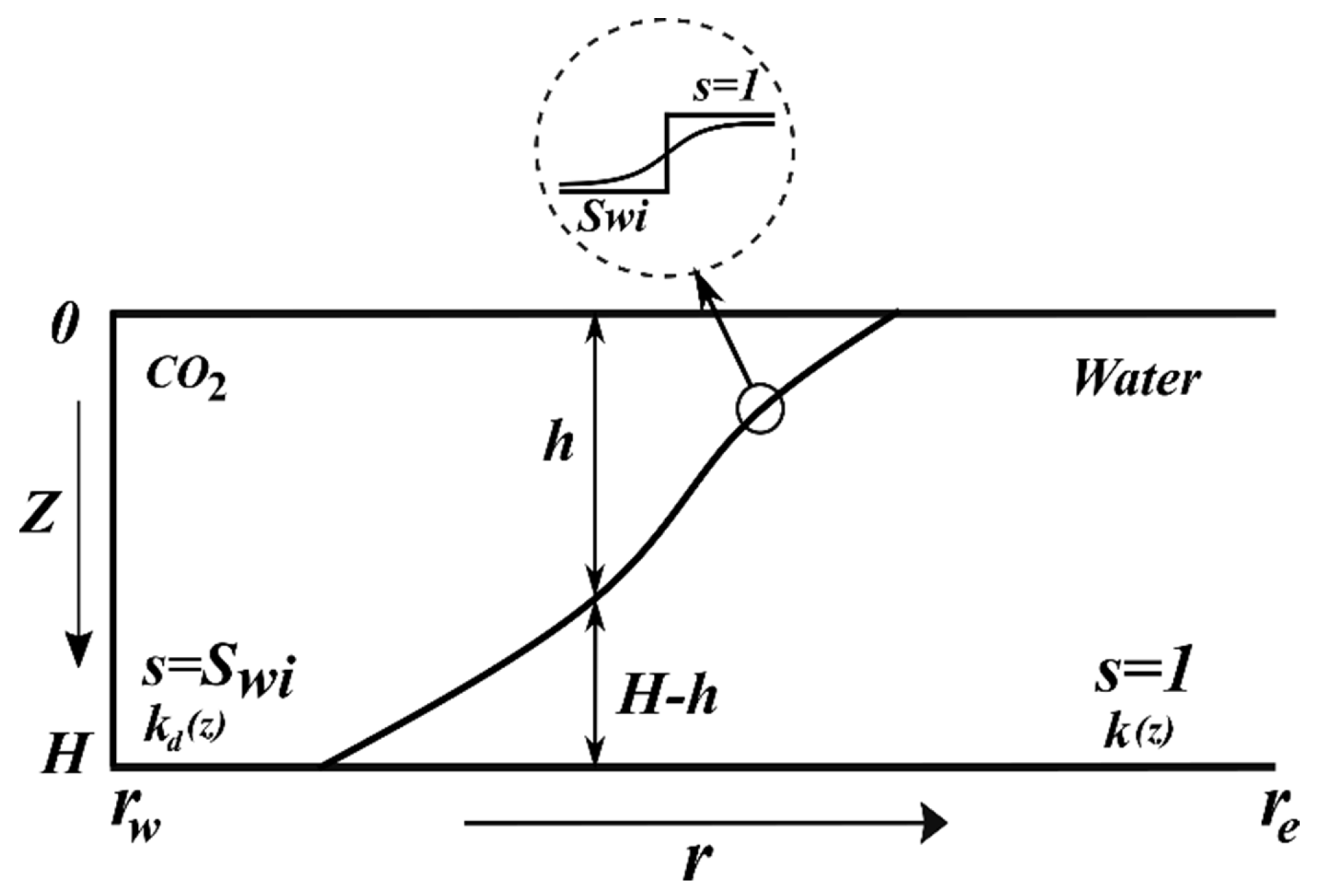
2. Mathematical Model for Quasi-2D Displacement with Formation Damage

This section develops a mathematical model for CO₂ injection into a layer-cake reservoir, accounting for CO₂-induced formation damage. It includes the model’s assumptions (Section 2.1), the governing equations for 2D flow (Section 2.2), and the averaged 1D model (Section 2.3).

2.1. Assumptions of the Model

We discuss CO₂ injection into a layer-cake reservoir, considering the inter-layer mass exchange. This mass exchange is assumed to be instantaneous, meaning the horizontal pressure gradient is independent of the vertical coordinate and is constant across the layers. Gravity and capillary pressure are ignored. Under viscous-dominant displacement, the filling of the layer by the injected gas occurs in accordance with the decrease in permeability [33,36]. While applying this model to a gravity-dominant case, gas zone consistently expands above the water zone.

Figure 1 illustrates the position of the water-gas contact, denoted as h = h(x,t), for the case in which the permeability decreases with depth, expressed as k_r = k(z). It is assumed that the vertical permeability, k_z, remains constant. The injected gas fills the layers from top to bottom. The permeability decreases from its initial value k(z) to the stabilised value k_d(z). This schematic is applicable to numerous displacement processes, where the surface h = h(x,t) separates the injected and displaced fluids. It is also assumed that no mass transfer occurs across the separating surface, implying that mass conservation is valid for both displacing and displaced fluids. In the case of CO₂ injection into water, water with saturation s = 1 moves ahead of the front, while gaseous CO₂ under the presence of connate water with dissolved CO₂ moves behind the front.

Various physical mechanisms can lead to changes in the injected phase permeability during enhanced oil recovery (EOR) or CO₂ injection. These include salt precipitation due to dry-out effect, hydrate resulting from temperature changes, detachment of clay and silica fines, and their straining in pores. Additionally, fines may be generated during rock dissolution in water in the presence of carbonic acid, and mineral precipitation may occur due to chemical reactions. Other factors include alteration in wettability, rock failure, precipitation of asphaltenes and paraffins, and polymer adsorption [34]. Our model assumes that the length of the transition zone, where permeability changes occur, is significantly shorter than the reservoir length. Therefore, at the reservoir scale, the permeability decline k(z) > k_d(z) is assumed to take place in immediate vicinity of the gas-water contact z = h(x,t). The present pseudo function model accounting for formation damage can be adopted for the above-mentioned field cases.

Consider a coreflood test using the core taken from a depth z, where the rock permeability changes from k(z) to k_d(z). Permeability stabilisation occurs after T_st pore volume injected (PVIs), resulting in a transition zone length equal to T_stl, where l is the core length. The condition for a thin transition zone length, which allows for the assumption of piston-like displacement in each layer and the existence of gas-water contact, is expressed as T_stl << L, where L is the reservoir length.

Displacement behaves in a piston-like manner within each layer. The initial water saturation in aquifer is equal to one, which corresponds to the saturation ahead of the piston. The saturation behind the front in the gas zone is denoted as S_wi. It is assumed that porosity remains constant with depth and that the displacement process does not alter porosity.

The dimensionless 2D formulation of the two-phase displacement includes three dimensionless groups: capillary–viscous, capillary–gravity, and aspect–anisotropy ratios. The conditions for the gravity-dominant case, expressed through relationships between those parameters, can be found in Yortsos [35], Kanevskaya [37], and Bedrikovetsky [30].

2.2. Governing 2D Equations

Consider two-phase unsteady state flow in two dimensions with coordinates (r, z, t). The governing equations for two-phase immiscible displacement include modified Darcy’s law in the r- and z-directions, along with mass balances for water and the total water-gas flux [30,31,38]:

$$u_{wr}=-{\displaystyle \frac{k(z)}{{\mu }_w}}{\displaystyle \frac{\mathsf{\partial }p}{\mathsf{\partial }r}},u_{gr}=-{\displaystyle \frac{k_d(z)K_{rgwi}}{{\mu }_g}}{\displaystyle \frac{\mathsf{\partial }p}{\mathsf{\partial }r}},u_{wz}=-{\displaystyle \frac{k_z}{{\mu }_w}}{\displaystyle \frac{\mathsf{\partial }p}{\mathsf{\partial }z}},u_{gz}=-{\displaystyle \frac{k_{zd}{K}_{rgwi}}{{\mu }_g}}{\displaystyle \frac{\mathsf{\partial }p}{\mathsf{\partial }z}}$$

(1)

$$\varphi r{\displaystyle \frac{\mathsf{\partial }s}{\mathsf{\partial }t}}+{\displaystyle \frac{\mathsf{\partial }(r{u}_{wr})}{\mathsf{\partial }r}}+{\displaystyle \frac{\mathsf{\partial }{u}_{wz}}{\mathsf{\partial }z}}=0,{\displaystyle \frac{\mathsf{\partial }(r{u}_r)}{\mathsf{\partial }r}}+{\displaystyle \frac{\mathsf{\partial }{u}_z}{\mathsf{\partial }z}}=0$$

(2)

$$\overrightarrow{u}={\overrightarrow{u}}_w+{\overrightarrow{u}}_g$$

(3)

Here, $\varphi$ is the porosity; u_wr and u_gr are the radial water and gas velocities, while u_wz and u_gz are the water and gas velocities in z direction. k(z) and k_d(z) represent the initial and damaged horizontal permeability profiles, respectively, and k_z and k_zd denote the initial and damaged vertical permeabilities. K_rgwi is the gas relative permeability at irreducible water saturation, and ${\mu }_w$ and ${\mu }_g$ are the water and gas viscosities. Substituting the four expressions for the velocity, as given by Equation (1), into the two mass balance equations (Equation (2)) yields a system of two equations for the two unknowns s(r,z,t) and p(r,z,t). Due to piston-like displacement in each layer, s = 1 and K_rw = 1 in the water zone, and s = S_wi in the gas zone.

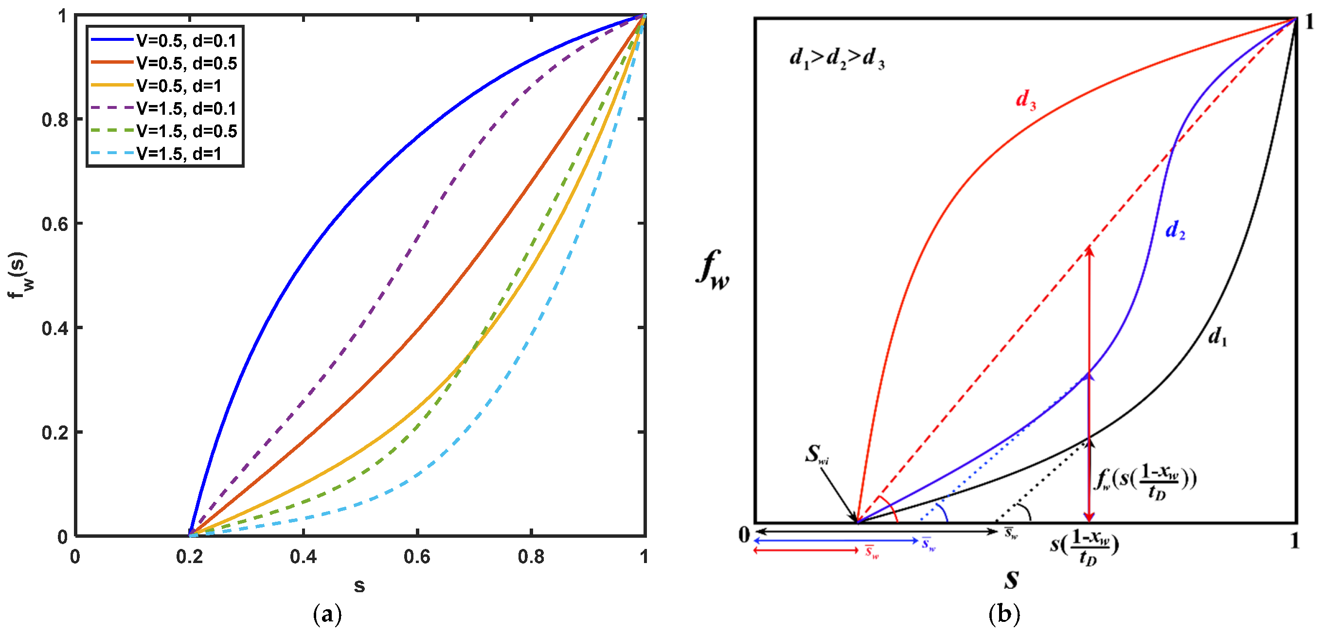
2.3. Dietz’s Model for Pseudo-Fractional Flow in a Layer-Cake Reservoir

Introduce the following dimensionless variables into Equations (1) and (2):

$$h_D={\displaystyle \frac{h}{H}}, z_D={\displaystyle \frac{z}{H}}, x_D={\left({\displaystyle \frac{r}{r_e}}\right)}^2, p_D={\displaystyle \frac{4\pi H\overline{k}}{q{\mu }_w}}p, t_D={\displaystyle \frac{qt}{\pi r_e^{2}H\varphi }}$$

(4)

Horizontal permeability is non-dimensionalized by its average value:

$$\overline{k}={\displaystyle \frac{1}{H}}{\displaystyle \underset{0}{\overset{H}{\int }}k(z)dz=}{\displaystyle \underset{0}{\overset{1}{\int }}k(z_D)d{z}_D,} k_D(z_D)={\displaystyle \frac{k(z_D)}{\overline{k}}}$$

(5)

The dimensionless Equations (1) and (2) in 1D, assuming no flux over the vertical z direction, become [30,31,38]:

$${\displaystyle \frac{\mathsf{\partial }s}{\mathsf{\partial }{t}_D}}+{\displaystyle \frac{\mathsf{\partial }{f}_w\left(s\right)}{\mathsf{\partial }{x}_D}}=0$$

(6)

$$1=-\mathsf{\Lambda }(s)x_D{\displaystyle \frac{\mathsf{\partial }{p}_D}{\mathsf{\partial }{x}_D}}$$

(7)

where the total mobility of two phases is

$$\mathsf{\Lambda }(s)=\left[{\displaystyle \frac{{\mu }_w{K}_{rgwi}d}{{\mu }_g}}{\displaystyle \underset{0}{\overset{\frac{1-s}{1-S_{wi}}}{\int }}{k}_D(z_D)d{z}_D}+{\displaystyle \underset{\frac{1-s}{1-S_{wi}}}{\overset{1}{\int }}{k}_D(z_D)d{z}_D}\right]$$

(8)

The initial condition for Equation (6) corresponds to a unit water saturation in the aquifer prior to injection.

$$t_D=0:s=1$$

(9)

The inlet boundary condition at the well corresponds to the irreducible water saturation.

$$x_D=x_w={\left({\displaystyle \frac{r_w}{r_e}}\right)}^2:s=S_{wi}$$

(10)

Let us determine the total mobility at the endpoints:

$$\{\begin{array}{ll}s=S_{wi}:& \mathsf{\Lambda }(s=S_{w_i})={\displaystyle \frac{{\mu }_w{K}_{rgwi}d}{{\mu }_g}}\\ s=1:& \mathsf{\Lambda }(s=1)=1\end{array}$$

(11)

Equation (11) defines the fluid mobilities corresponding to the initial and boundary conditions specified by Equations (9) and (10), respectively. The fractional flow curve f_w(s) is given by Equation (A4). Figure 2 presents the plots of fractional flow curves (FFCs) for different values of heterogeneity variation V as defined by Equation (12), and for the permeability damage factor d, presented in Equation (13).

$$V={\displaystyle \frac{k_{\max }-k_{\min }}{\overline{k}}}$$

(12)

$$d(z)={\displaystyle \frac{k_d(z)}{k(z)}}$$

(13)

Figure 2 shows the case in which the permeability damage factor d is constant. A lower damage factor results in higher hydraulic resistance for gas (leading to a reduced gas flux), and, consequently, a higher fractional flow of water. Greater variability in heterogeneity implies increased heterogeneity, greater variability in velocities f’_w(s), and more curvilinear FFCs. Depending on the level of heterogeneity and damage factor, the FFC may be concave, convex, or S-shaped.

3. Analytical Model

This section presents the exact solution for the quasi-2D displacement problem with induced formation damage (Section 3.1), calculates the sweep coefficient (Section 3.2), and provides the derivations for well impedance and skin factor (Section 3.3).

3.1. Self-Similar Solution

Substituting the coordinate x_D into solution (A12) leads to the exact solution of the initial-boundary value problem defined by Equations (6), (9) and (10), as follows [30,31,38]:

$$s\left(x_D,t_D\right)=\{\begin{array}{cc}{S}_{wi},& 0<{\displaystyle \frac{x_D-x_w}{t_D}}<D_i\\ {\displaystyle \frac{x_D-x_w}{t_D}}=f_w^{\prime }\left(s\right),& D_i<{\displaystyle \frac{x_D-x_w}{t_D}}<D_f\\ 1,& D_f<{\displaystyle \frac{x_D-x_w}{t_D}}<\infty \end{array}$$

(14)

Here, the velocities of the water-gas front and rear water front, respectively, are the following

$$D_i=f_w^{\prime }\left(S_{wi}\right), D_f=f_w^{\prime }\left(s_f\right)={\displaystyle \frac{1-f_w\left(s_f\right)}{1-s_f}}$$

(15)

The mathematical fundamentals for the self-similar solutions of the Riemann problems, such as Equations (6), (9), (10) and (14), can be found in the works of Dietz [25], Hearn [26], and Polyanin and Zaitsev [39].

Figure 3 illustrates the graphical construction of the solution given by Equation (14) and the structure of the displacement zone. Figure 3b depicts the turned plane (s,(x_D-x_w)/t_D) and the profile s = s((x_D − x_w)/t_D), which remains identical to the profile s = s(x_D) when t_D = 1, i.e., after 1 PVI. The three elements of the solution in Equation (14) correspond to three zones in the (x_D, t_D) plane (Figure 3c), three intervals in profile s(x_D,t_D = 1) (Figure 3b) and three elements: point S_wi, segment S_wi − s_f, and point s = 1 on the FFC (Figure 3a).

Consider small time t₁ and the movement from the injection well at x_D = x_w, t_D = t₁ to x_D = 1, t_D = t₁ along the horizontal line in Figure 3c. The variation of the position x_D from x_w of the wellbore to drainage boundary corresponds to constant saturation s = S_wi in zone II, an increase from S_wi to s = s_f in zone I, and constant saturation s = 1 in zone 0. This sequence corresponds to “staying” at point s = S_wi, moving along the segment S_wi − s_f, and making a jump to the point s = 1 in the plane (s,f_w(s)).

Figure 2 shows different forms of the flow function f_w(s), which result in the appearance of several saturation jumps in the solution s(x_D,t_D) [23,35,40].

3.2. Average Water Saturation and Sweep Coefficient

Now, we present the expression for the average water saturation $\overline{s}(t_D)$ using the exact solution from Equation (14).

$$\overline{s}(t_D)={\displaystyle \underset{x_w}{\overset{1}{\int }}s(x_D,t_D)d{x}_D}$$

(16)

Appendix C presents the detailed derivations for average water saturation across three distinct stages: (1) before the arrival of the water-gas front, (2) after the arrival of the water-gas front but before the arrival of the rear water front, and (3) after the arrival of the rear water front. The explicit expression for average water saturation as a function of time is the following:

$$\overline{s}(t_D)=\{\begin{array}{ll}(1-x_w)-t_D& 0<t_D<{\displaystyle \frac{1-x_w}{D_f}}\\ (1-x_w)s({\displaystyle \frac{1-x_w}{t_D}})-t_{D}f(s({\displaystyle \frac{1-x_w}{t_D}}))& {\displaystyle \frac{1-x_w}{D_f}}<t_D<{\displaystyle \frac{1-x_w}{D_i}}\\ (1-x_w)S_{wi}& {\displaystyle \frac{1-x_w}{D_i}}<t_D<\infty \end{array}$$

(17)

3.3. Impedance and Skin Factor Calculations

Formation damage to a well can be expressed in terms of impedance, which is the normalised reciprocal of the injectivity index [30,31,38], as shown in Equation (18), or via the skin factor [41], as indicated in Equation (19).

$$J(t_D)={\displaystyle \frac{II(t_D=0)}{II(t_D)}}={\displaystyle \frac{q(t_D=0)}{\Delta p_D(t_D=0)}}{\displaystyle \frac{\Delta p_D(t_D)}{q(t_D)}}$$

(18)

$$\Delta p_D(t_D)={\displaystyle \frac{{\mu }_{g}q(t_D)}{2\pi k}}\left(\ln {\displaystyle \frac{r_e}{r_w}}+S(t_D)\right),S(t_D)=\left[J(t_D)-1\right]\ln {\displaystyle \frac{r_e}{r_w}}$$

(19)

The detailed derivations of well impedance for three moments—before the arrival of the water-gas front, after the arrival of the water-gas front but before the arrival of the rear water front, and after the arrival of rear water front—are provided in Appendix D. The explicit expression for well impedance as a function of time is the following:

$$J(t_D)=\{\begin{array}{ll}-{\displaystyle \frac{{\mu }_g}{{\mu }_w{K}_{rgwi}d}}{\displaystyle \frac{\ln \left(\frac{D_i{t}_D+x_w}{x_w}\right)}{\ln (x_w)}}-{\displaystyle \frac{1}{\ln (x_w)}}{\displaystyle \underset{S_{wi}}{\overset{1}{\int }}\frac{f_w^{″}\left(s\right)ds}{\left(f_w^{\prime }\left(s\right)+\frac{x_w}{t_D}\right)\mathsf{\Lambda }\left(s\right)}}+{\displaystyle \frac{\ln (D_f{t}_D+x_w)}{\ln (x_w)}}& 0<t_D<{\displaystyle \frac{1-x_w}{D_f}}\\ -{\displaystyle \frac{{\mu }_g}{{\mu }_w{K}_{rgwi}d}}{\displaystyle \frac{\ln \left(\frac{D_i{t}_D+x_w}{x_w}\right)}{\ln (x_w)}}-{\displaystyle \frac{1}{\ln (x_w)}}{\displaystyle \underset{S_{wi}}{\overset{s(t_D)}{\int }}\frac{f_w^{″}\left(s\right)}{\left(f_w^{\prime }\left(s\right)+\frac{x_w}{t_D}\right)\mathsf{\Lambda }\left(s\right)}}ds& \frac{1-x_w}{D_f}<t_D<\frac{1-x_w}{D_i}\\ {\displaystyle \frac{{\mu }_g}{{\mu }_w{K}_{rgwi}d}}& {\displaystyle \frac{1-x_w}{D_i}}<t_D<\infty \end{array}$$

(20)

The initial dimensionless pressure drop is given by Equation (21).

$$\Delta p_D(0)=-\ln (x_w)$$

(21)

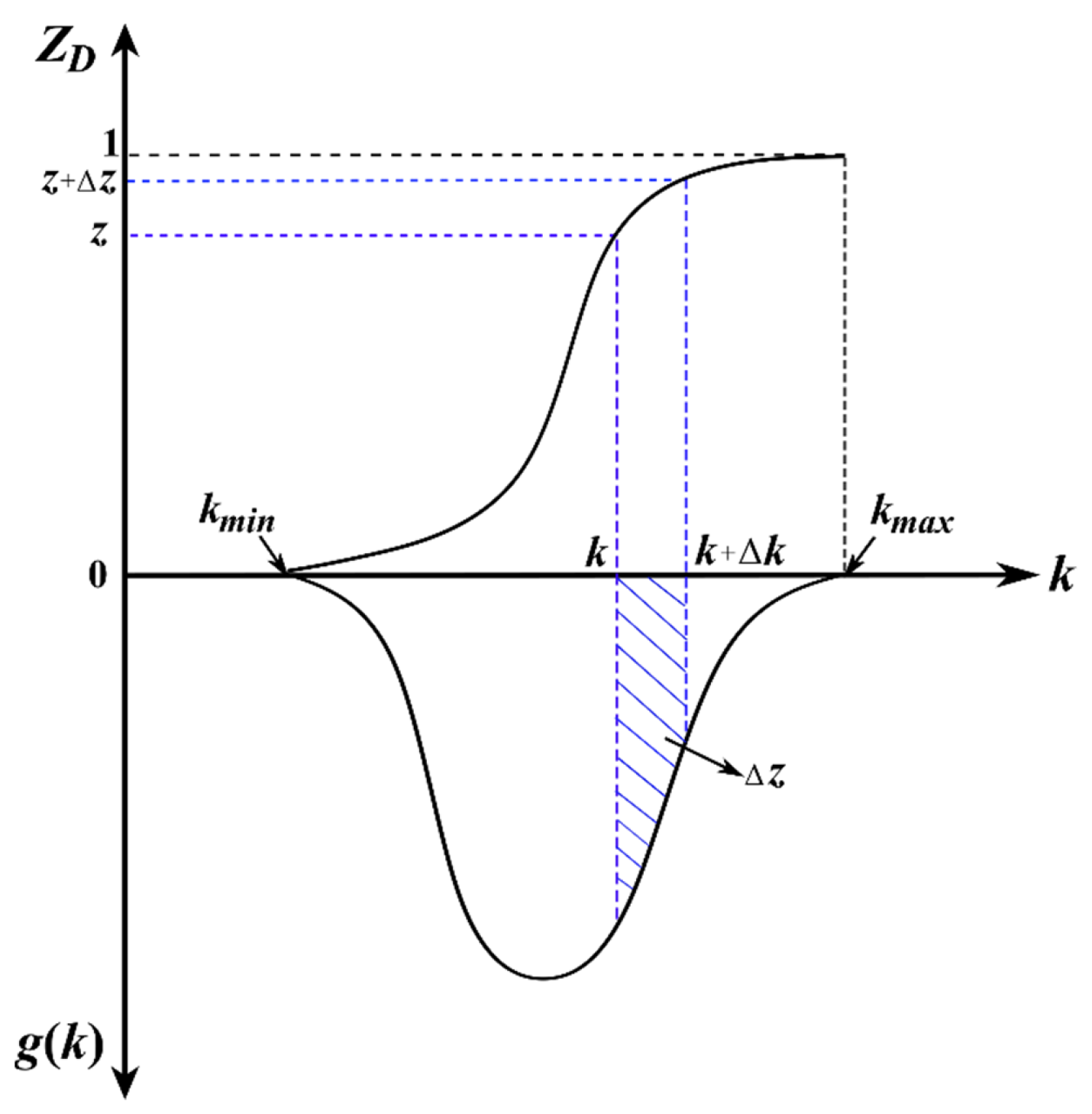
4. Practical Calculations: Power-Law Permeability Profiles

Consider the probability distribution function (PDF) or histogram of permeability, denoted as g(k). This function characterises the likelihood of different permeability values within a given reservoir or geological formation. The shape of the distribution provides insight into the variability and range of permeability throughout the medium, which can significantly influence fluid flow behaviour during processes such as CO₂ injection or hydrocarbon extraction. The corresponding permeability profile k(z) represents how permeability varies with depth in the reservoir. By integrating g(k), the permeability profile can be constructed to illustrate the spatial distribution of permeability values at different depths throughout the vertical extent of the reservoir, as follows:

$$z={\displaystyle \underset{k}{\overset{k_{\max }}{\int }}g(y)dy,\frac{dk}{dz}=-\frac{1}{g(k)}}$$

(22)

The mono-modal PDF for permeability, shown in Figure 4, indicates that the probability of permeability values reaches zero at the minimum and maximum permeability limits, k = k_min and k = k_max, respectively. According to Equation (22), the slope of the permeability profile k = k(z) becomes infinitely steep at these boundary points. This behaviour is illustrated in Figure 4, where the profile sharply ascends or descends as it approaches k_min and k_max. The permeability profile that satisfies these conditions is given by the following equation:

$$\{\begin{array}{l}k\left(z_D\right)=k_{\min }-\left(k_{\min }-k_{\max }\right)b\left(z_D\right)\\ b\left(z_D\right)=\{\begin{array}{cc}1-a{z_D}^n,& 0<z_D={\displaystyle \frac{z}{H}}<c\\ {\displaystyle \frac{1-a{c}^n}{{\left(1-c\right)}^m}}{\left(1-z_D\right)}^m,& c<z_D={\displaystyle \frac{z}{H}}<1\end{array}\end{array}$$

(23)

The average permeability, calculated using the profile provided in Equation (23), can be obtained as follows:

$$\overline{k}=k_{\min }-\left(k_{\min }-k_{\max }\right)\left((c-{\displaystyle \frac{a{c}^{n+1}}{n+1}})+{\displaystyle \frac{1-a{c}^n}{m+1}}\left(1-c\right)\right)$$

(24)

Equation (24) enables the expression of the heterogeneity variation V, as defined by Equation (12), in terms of the parameters a, c, m, and n of the power-law permeability profile, as follows:

$$V={\displaystyle \frac{1}{\left(\frac{k_{\min }}{k_{\max }-k_{\min }}\right)+\left((c-\frac{a{c}^{n+1}}{n+1})+\frac{1-a{c}^n}{m+1}\left(1-c\right)\right)}}$$

(25)

Substituting the permeability profile from Equation (23) into the fractional flow (Equation (A4)) and total mobility (Equation (8)) equations leads to expressions that account for different conditions of gas height h and the inflection point c within the power-law profile. Detailed derivations for fractional flow and total mobility within this framework can be found in Appendix E and Appendix F. To enhance clarity regarding the transition from equation derivations to their practical implications, Figure 5 illustrates the various steps involved in implementing the developed models in this study.

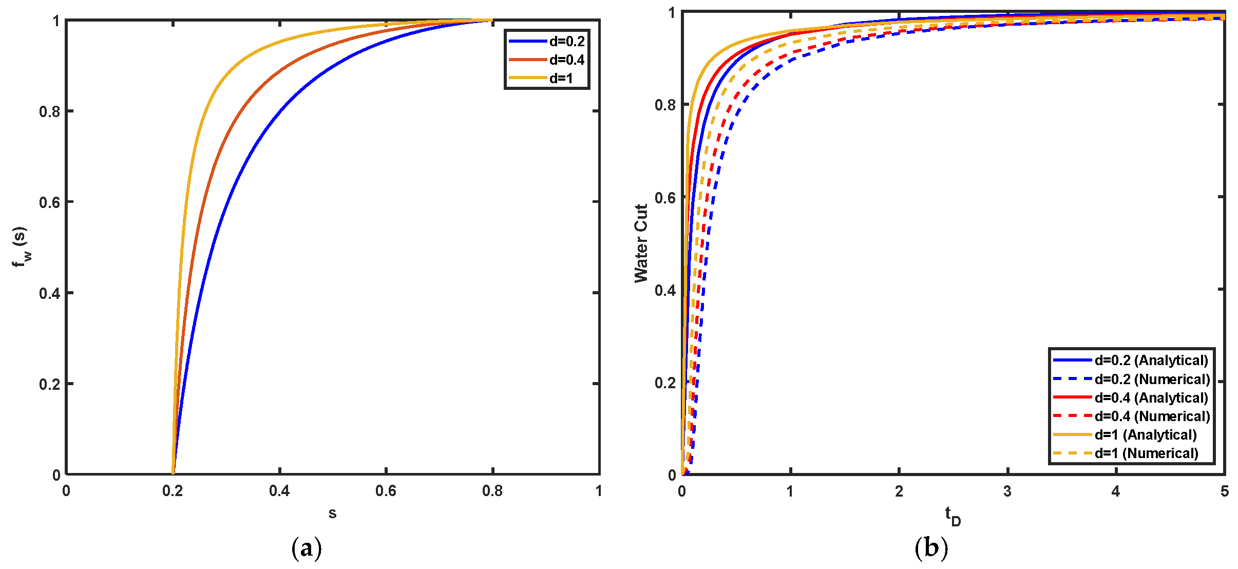
5. Validation of the Analytical Model

The extended Dietz’s model, which accounts for formation damage and is represented by Equations (6)–(8), is derived for any two-phase flow with a decrease in permeability behind the displacement front. This includes all mobility-control EOR methods. To validate the model, we consider low-salinity water flooding in the layer-cake oil reservoir.

The permeability increases from 10 mD at the bottom to 500 mD at the top of the reservoir, which has a thickness of 15 m. The distance between the injectors and producers is 1000 m. The viscosities of oil, water, and low-salinity water are 50 cp, 1 cp, and 1.2 cp, respectively. The densities of oil and water are 700 kg/m³ and 1000 kg/m³, respectively. The Corey coefficients for oil-water are as follows: S_wi = 0.2, S_or = 0.2, K_rwor = 0.3, K_rowi = 0.8, n_w = 3.0 and n_o = 1.5. Formation damage is assumed to occur due to detachment, migration, and straining of the natural reservoir fines. Figure 6a,b present the fractional flow and water-cut curves, respectively, corresponding to formation damage factors d = 0.2, 0.4, and 1.0 (blue, red, and yellow curves). The case where d = 1 corresponds to damage-free waterflooding. The dashed and solid curves reflect numerical and analytical modelling results, respectively. The coefficients of determination for the cases d = 0.2, 0.4, and 1.0, are 0.987, 0.978, and 0.977, respectively. So, the deviation between numerical and pseudo-function models typically falls within established error intervals. Discrepancies between the numerical and analytical solutions are due to the simplification assumptions of the analytical model [35].

The pseudo functions, used in this paper, do not represent exact solutions of 2D equations; rather, they correspond to asymptotic cases [29,30,31,32,33,36,38,39,41,42,43]. In particular, Dietz’s pseudo functions, as represented by Equations (A1) and (A2), reflect the case of gravity domination, where viscous forces significantly exceed both capillary and gravity forces [34]. Despite the widespread application of pseudo-relative permeability models in reservoir engineering, a close match between numerical and analytical solutions is not expected. It is important to emphasise that analytical pseudo-function models should not be considered as benchmarks for numerical models [37,44]. Pseudo-relative permeability models are used for sensitivity analysis studies to determine general tendencies and orders of magnitude. Indeed, Figure 6a,b demonstrate a decrease in fractional flow functions with an increase in formation damage, leading to an enhancement of the sweep coefficient. The absolute increase in fractional flow due to the increase in formation damage is of the same order of magnitude for both numerical and analytical models—the distances between the analytical curves (represented by continuous lines) and the numerical curves (represented by dashed lines) corresponding to the same d-values are consistently similar, indicating a robust validation in this study.

6. Results of Analytical Modelling

Here, we present the sensitivity study regarding the turning-point parameter c and heterogeneity variation V. Figure 7 shows the effect of changes in the turning-point parameter c on the permeability profile (Figure 7a) and FFC (Figure 7b). The lower the value of c, the more homogeneous the reservoir becomes. However, the impact of c on FFC is negligible, which is an advantage when selecting Equation (23) for the permeability profile k(z).

Figure 8 presents the effect of heterogeneity variation V on the permeability profile and the FFC. An increase in V within the conventional interval results in significant increase in reservoir heterogeneity. Figure 8a shows the variation of V under constant average permeability, where all curves intersect at a single point. As V increases, the variation in permeability also increases. The higher the V value, the greater the velocity dispersion, resulting in a more curvilinear FFC (Figure 8b). This leads to an increase in the thickness of the CO₂-water mixture zone and a decrease in sweep efficiency.

The sensitivity of coefficient c, heterogeneity variation V, and damage factor d on the history of averaged gas saturation is presented in Figure 9. Figure 7 demonstrates a negligible effect of c on FFC, which consequently results in a negligible effect of c on the average gas saturation history (Figure 9a). In contrast, Figure 8 shows a significant effect of V on FFC, indicating that the saturation history is also affected. Specifically, Figure 9b illustrates that higher values of V yield a faster CO₂-water front, a lower breakthrough moment, a lower full-displacement moment, a larger mixture zone, and a lower gas saturation. As V increases from 0.1 to 1.5, the average gas saturation at t_D = 1 PVI decreases from 0.75 to 0.65. The average gas saturation at the moment t_D = 1 PVI corresponds to the sweep coefficient, which indicates the fraction of the reservoir volume filled by the injected CO₂. The capture of CO₂ by the rock due to dissolution in water, chemical reactions, capillary forces, and stratigraphic entrapment occurs specifically within the swept volume.

Figure 9c shows that as the damage factor d decreases, the average gas saturation increases. With d decreasing from 2.0 to 0.1, the average gas saturation at t_D = 1 PVI rises from 0.5 to 0.8. This can be explained by the deceleration of gas due to permeability damage, which decrease gas mobility and increases sweep as a result.

Figure 10a shows the impact of heterogeneity V on the stabilization time, defined as the number of PVIs required for saturation to reach S_wi uniformly across the reservoir. As the value of V increases, the velocity of the characteristic line carrying s = S_wi [45,46] decreases, resulting in a delayed complete displacement. Figure 10b indicates that greater reservoir heterogeneity corresponds to a faster breakthrough.

Sweep efficiency is the primary parameter determining the storage capacity. Figure 11 shows that as the formation damage factor d decreases, gas deceleration increases, resulting in higher sweep efficiency. Conversely, greater reservoir heterogeneity V leads to a reduction in sweep efficiency.

The primary parameter determining the injectivity decline during CO₂ injection is the formation damage factor d. Let us define the impedance that reflects this feature. The dimensionless pressure drop (impedance) J(t_D) is defined by Equation (18). Figure 12 illustrates that as the coefficient d decreases, the impedance increases. For high value d > 1, which corresponds to an increase in permeability, J(t_D) decreases. This effect is depicted in Figure 12, where J(t_D) decreases at high d and increases at lower d. Therefore, there exists a critical d value (d_c) at which these two aforementioned effects compensate for each other, resulting in the impedance remaining equal to one.

For fines migration during CO₂ injection, the formation damage factor d typically varies within the narrow interval 0.4–0.5 [25,31]. However, Tan et al. [47] reported a wider variation of d, ranging from 0.2 to 0.9. For salt precipitation, d varies from 0.3 to 0.8 [38,39,48]. In the context of CO₂ injection into oilfields with asphaltene precipitation, the formation damage factor varies from 0.2 to 0.9 [47,49,50]. In most coreflood tests, the majority of the permeability decline occurs within less than 1000 PVIs [51]. Polymer and surfactant floods manage to reach residual oil throughout the core after 3 to 10 PVIs [52]. For a core length of 5 cm, this corresponds to a mixture zone of 50 m (calculated as 50 = 0.05 × 1000). Therefore, the length of the mixture zone is significantly smaller than the reservoir size, thus the assumptions of the extended Dietz’s model are fulfilled.

The above-mentioned sensitivity analysis demonstrates that heterogeneity variation V significantly impacts CO₂ storage performance. Understanding how heterogeneity variation V affects velocity dispersion, breakthrough times, and sweep efficiency is crucial for accurately characterising reservoir heterogeneity and optimising injection strategies. Moreover, managing the formation damage d can enhance sweep efficiency and injectivity, which are critical for maximising storage capacity and ensuring efficient CO₂ injection. These insights enable more informed decision-making in the design and implementation of CO₂ storage projects, ensuring effective and efficient long-term storage.

7. Field Case

This section presents the application of analytical modelling for calculating sweep efficiency and well index, as specified in Equations (17) and (20), across three reservoirs in formation L (Malaysia). This field is located offshore at a depth of 60 m. The porosity ranges from 0.20 to 0.27, while the mean permeability varies from 64 mD to 320 mD. The gas reservoir with weak aquifer support has been depleted by 21 production wells. The reservoir pressure decreased from 2100 to 600 psia, with an average gas recovery of 78%. The gas reservoir contains 13% CO₂, and the depositional environment is characterised as shallow marine clastic. Three reservoir facies have been identified: massive sandstone, laminated sandstone, and mudstone. We discuss three reservoirs, labelled A, B, and C, within field L. The basic reservoir properties and corresponding statistical parameters of permeability distribution for these reservoirs are presented in the Supplementary Material. The permeability distribution profiles for reservoirs A and C are approximated using a power-law function, with the minimum least squared error, as shown in Figure 13. The permeability distribution for Reservoir B can also be found in the Supplementary Material. The results indicate that the permeability histograms for all reservoirs follow a log-normal distribution with high accuracy

Figure 14 presents the plots of sweep efficiency and impedance for Reservoirs A and C, with the results for Reservoir B available in the Supplementary Material. The analysis confirms the key theoretical conclusions regarding sweep efficiency and damage growth, which have been previously discussed (refer to Figure 9, Figure 10, Figure 11 and Figure 12). Notably, the findings indicate that a greater reduction in permeability resulting from CO₂ injection leads to an increase in the skin factor, which enhances sweep efficiency. Based on Figure 14a,b, as the damage factor d decreases from 1 to a critical value of 0.016, significant improvements in sweep efficiency are observed across all reservoirs. Specifically, for Reservoir A, the sweep coefficient rises from 1% to 53%; for Reservoir B, it increases from 3% to 53%; and for Reservoir C, it escalates from 7% to 50%. These results underscore the significant influence of permeability damage on enhancing the sweep efficiency of CO₂ injection. Moreover, the stabilised impedance exhibits a consistent increasing trend as the damage factor d decreases across all reservoirs under consideration. Specifically, for Reservoir A, the stabilised impedance rises from 0.22 to 1; for Reservoir B, it increases from 0.23 to 1; and for Reservoir C, it grows from 0.20 to 1. These findings collectively highlight the significant influence of the damage factor d on sweep efficiency and well injectivity, suggesting the existence of an optimised damage factor d that maximises CO₂ storage while maintaining practical injection pressures.

8. Discussions

Regarding the extension of the model, the limitations and applicability of Dietz’s model have been extensively discussed in the literature [53]. In particular, the model is valid at high velocities, where the injected phase is forced into highly permeable layers, which occurs under viscous domination near the injectors. Conversely, gravity predominates at low velocities, far away from the injection wells, where stratified flow of gas occurs above water. The model represented by Equations (6)–(8) can be applied to the case of gravity domination.

This paper introduces permeability damage into Dietz’s model to examine CO₂ injection into aquifers where the initial water saturation is equal to one. The model is also applicable to completely depleted gas fields, where the initial water saturation is equal to that of residual gas S_gr. Furthermore, the model can be applied to any two-phase displacement with induced formation damage, such as CO₂ injection into oilfields accompanied by asphaltene precipitation or chemical EOR. It is assumed that the transition zone length is significantly smaller than the reservoir size, allowing for a complete jump across the displacement front in the layer-cake model.

The model, represented by Equations (6) and (7), assumes constant porosity in the reservoir throughout the entire injection period. However, this assumption is not valid for hydrate formation and asphaltene precipitation that occur during CO₂ injection. Porosity variations behind the front can be incorporated in the model, similar to how it was introduced into the damage-free Dietz’s model in Bedrikovetsky [30]. This represents the next step in the development of the model, represented by Equations (6) and (7).

Dietz’s model (Equations (6) and (7)) demonstrates independence of the upscaled pseudo-relative permeability from velocity. Here, we discuss the radial flow problem, in which flow velocity varies with radius, so the velocity dependence of the relative permeability is important [38,54,55]. Different upscaling methods yield calculations for the so-called rate-dependent relative permeability [30,31]. The method outlined in Equations (A1) to (A4) allows the incorporation of formation damage into Dietz’s model with velocity-dependent endpoint-relative permeability and saturations.

In relation to the model validation conducted in this study, the present model integrates permeability damage into the classical pseudo-function models—specifically, Dietz’s viscous-dominant and gravity-dominant systems. These models have been thoroughly validated without formation damage, and the results have been extensively documented in the literature, including references [28,29,30,31,32,34,35,36,37]. The scenario of low-salinity waterflooding, in which permeability reduces at the water-oil interface due to fines migration, reflects the difference between our model and classical models. Consequently, we utilised this scenario to validate our model.

Regarding the connections to CO₂ coreflooding, the abrupt decrease in permeability within each layer is characterised by a change from the initial permeability, k(z), to the final permeability, k_d(z), behind the piston-like front. This change is assumed to occur close to the displacement front in each layer, meaning that the length of the mixture zone is significantly smaller than the reservoir length. In a typical laboratory test corresponding to a rock sample with depth z and an initial permeability of k(z), the final permeability k_d(z) stabilises within a period of less than 1000 PVIs. For a core length of 5 cm, this stabilisation corresponds to a mixture length of 50 m, which is also expected to be significantly smaller than the reservoir length.

Regarding the matching of the reservoir model with near-well damage, the model considers in situ permeability damage k(z)→k_d(z) within the reservoir. It can also accommodate the formation damage occurring close to injectors, such as salt precipitation in dried-out zones due to capillary backflow during CO₂ injection [30], generation of fines due to rock drying [56], or deep bed filtration and external filter cake formation during waterflooding [57]. The criterion for near-well damage is that the formation damage zone’s radius is significantly smaller than the drainage radius [44]. The analytical solutions for 1D radial formation damage problems, obtained in the aforementioned works, yield explicit expressions for the skin factor, which adds into the inlet-pressure boundary condition presented in Equations (18) and (19). This matched asymptotic expansion was performed for waterflooding with colloidal particles by Kalantariasl et al. [45] and can be performed for any quasi-2D reservoir model with upscaled pseudo-phase permeability and an analytical model for well injectivity damage. Reliable analytical modelling is essential for preventing and mitigating formation damage [46,58]. In the context of CO₂ injection, this pertains to the injection of nanofluids and wet or hot CO₂ [59].

The current model provides a robust foundation for understanding CO₂ flow dynamics during injection in subsurface heterogeneous systems. However, several opportunities for enhancement exist that could improve its predictive accuracy. One key area for improvement is the incorporation of the rate dependency of the fractional flow function, particularly in scenarios involving fast gas flows, where the Forchheimer law may be more applicable than Darcy’s law. Additionally, considering the behaviour of non-Newtonian fluids could yield more precise flow predictions. Furthermore, while integrating complex chemical interactions—such as mineral precipitation and other reactions contributing to CO₂ capture in the swept zone—may increase the model’s complexity, it can significantly enrich the mathematical framework. By addressing these factors, the model can produce results that more accurately reflect the complexities of real-world systems, thereby enhancing its applicability and relevance in the field.

9. Conclusive Remarks

The paper presents an analytical model for two-phase displacement in layer-cake reservoirs, considering formation damage due to CO₂ injection in cases of gravity-dominant flows. The extension of Dietz’s model for gravity-dominated floods allows for considering permeability damage caused by injection. A key assumption is that the permeability change after injection in each layer is equivalent to that observed in the corresponding coreflood tests, implying that the permeability ahead and behind the displacement front in each layer are obtained from lab corefloods. Another assumption is that the time taken for the displacement front to pass through the transition zone is significantly shorter than the injection period.

The analytical model allows the derivation of the explicit formulae for well impedance, skin factor, and the evolution of sweep coefficient during the accumulation of formation damage induced by the injection. It allows for fast and effective methods for predicting well and reservoir behaviour.

The higher the induced formation damage, the higher the well impedance and skin factor of the injection well, as well as the sweep coefficient, which arises from the additional hydraulic resistance created against the injected gas. Consequently, formation damage increases gas storage capacity of the geological formation. While formation damage is typically known for its detrimental effect on projects due to well injectivity decline, it can also enhance sweep efficiency and positively influence the reservoir’s performance.

References

1. Nassan, T.H.; Freese, C.; Baganz, D.; Alkan, H.; Burachok, O.; Solbakken, J.; Zamani, N.; Aarra, M.G.; Amro, M. Integrity Experiments for Geological Carbon Storage (GCS) in Depleted Hydrocarbon Reservoirs: Wellbore Components under Cyclic CO2 Injection Conditions. Energies 2024, 17, 3014. [Google Scholar] [CrossRef]
2. Song, Y.; Jun, S.; Na, Y.; Kim, K.; Jang, Y.; Wang, J. Geomechanical challenges during geological CO2 storage: A review. Chem. Eng. J. 2023, 456, 140968. [Google Scholar] [CrossRef]
3. Zhang, Y.; Jackson, C.; Krevor, S. An Estimate of the Amount of Geological CO2 Storage over the Period of 1996–2020. Environ. Sci. Technol. Lett. 2022, 9, 693–698. [Google Scholar] [CrossRef]
4. Ngata, M.R.; Yang, B.; Aminu, M.D.; Iddphonce, R.; Omari, A.; Shaame, M.; Nyakilla, E.E.; Mwakateba, I.A.; Mwakipunda, G.C.; Yanyi-Akofur, D. Review of Developments in Nanotechnology Application for Formation Damage Control. Energy Fuels 2022, 36, 80–97. [Google Scholar] [CrossRef]
5. Ngata, M.R.; Yang, B.; Aminu, M.D.; Emmanuely, B.L.; Said, A.A.; Kalibwami, D.C.; Mwakipunda, G.C.; Ochilov, E.; Nyakilla, E.E. Minireview of Formation Damage Control through Nanotechnology Utilization at Fieldwork Conditions. Energy Fuels 2022, 36, 4174–4185. [Google Scholar] [CrossRef]
6. Sbai, M.A.; Azaroual, M. Numerical modeling of formation damage by two-phase particulate transport processes during CO2 injection in deep heterogeneous porous media. Adv. Water Resour. 2011, 34, 62–82. [Google Scholar] [CrossRef]
7. Tang, Y.; Hu, S.; He, Y.; Wang, Y.; Wan, X.; Cui, S.; Long, K. Experiment on CO2-brine-rock interaction during CO2 injection and storage in gas reservoirs with aquifer. Chem. Eng. J. 2021, 413, 127567. [Google Scholar] [CrossRef]
8. Liu, B.; Zhao, F.; Xu, J.; Qi, Y. Experimental Investigation and Numerical Simulation of CO2–Brine–Rock Interactions during CO2 Sequestration in a Deep Saline Aquifer. Sustainability 2019, 11, 317. [Google Scholar] [CrossRef]
9. Khurshid, I.; Choe, J. Analyses of thermal disturbance and formation damages during carbon dioxide injection in shallow and deep reservoirs. Int. J. Oil Gas Coal Technol. 2016, 11, 141–153. [Google Scholar] [CrossRef]
10. Baklid, A.; Korbol, R.; Owren, G. Sleipner Vest CO2 Disposal, CO2 Injection into a Shallow Underground Aquifer. In Proceedings of the SPE Annual Technical Conference and Exhibition 1996, Denver, CO, USA, 6–9 October 1996. [Google Scholar]
11. Eiken, O.; Ringrose, P.; Hermanrud, C.; Nazarian, B.; Torp, T.A.; Høier, L. Lessons learned from 14 years of CCS operations: Sleipner, In Salah and Snøhvit. Energy Procedia 2011, 4, 5541–5548. [Google Scholar] [CrossRef]
12. Hansen, O.; Gilding, D.; Nazarian, B.; Osdal, B.; Ringrose, P.; Kristoffersen, J.-B.; Eiken, O.; Hansen, H. Snøhvit: The History of Injecting and Storing 1 Mt CO2 in the Fluvial Tubåen Fm. Energy Procedia 2013, 37, 3565–3573. [Google Scholar] [CrossRef]
13. Ringrose, P.S.; Mathieson, A.S.; Wright, I.W.; Selama, F.; Hansen, O.; Bissell, R.; Saoula, N.; Midgley, J. The In Salah CO2 Storage Project: Lessons Learned and Knowledge Transfer. Energy Procedia 2013, 37, 6226–6236. [Google Scholar] [CrossRef]
14. Bjørnarå, T.I.; Bohloli, B.; Park, J. Field-data analysis and hydromechanical modeling of CO2 storage at In Salah, Algeria. Int. J. Greenh. Gas Control 2018, 79, 61–72. [Google Scholar] [CrossRef]
15. Ringrose, P. How to Store CO2 Underground: Insights from Early-Mover CCS Projects; Springer International Publishing: Berlin/Heidelberg, Germany, 2020. [Google Scholar]
16. Smith, N.; Boone, P.; Oguntimehin, A.; van Essen, G.; Guo, R.; Reynolds, M.A.; Friesen, L.; Cano, M.-C.; O’Brien, S. Quest CCS facility: Halite damage and injectivity remediation in CO2 injection wells. Int. J. Greenh. Gas Control 2022, 119, 103718. [Google Scholar] [CrossRef]
17. Russell, T.; Wong, K.; Zeinijahromi, A.; Bedrikovetsky, P. Effects of delayed particle detachment on injectivity decline due to fines migration. J. Hydrol. 2018, 564, 1099–1109. [Google Scholar] [CrossRef]
18. Chequer, L.; Nguyen, C.; Loi, G.; Zeinijahromi, A.; Bedrikovetsky, P. Fines migration in aquifers: Production history treatment and well behaviour prediction. J. Hydrol. 2021, 602, 126660. [Google Scholar] [CrossRef]
19. Ge, J.; Zhang, X.; Le-Hussain, F. Fines migration and mineral reactions as a mechanism for CO2 residual trapping during CO2 sequestration. Energy 2022, 239, 122233. [Google Scholar] [CrossRef]
20. Ge, J.; Zhang, X.; Liu, J.; Almutairi, A.; Le-Hussain, F. Influence of capillary pressure boundary conditions and hysteresis on CO2-water relative permeability. Fuel 2022, 321, 124132. [Google Scholar] [CrossRef]
21. Wang, Y.; Bedrikovetsky, P.; Yin, H.; Othman, F.; Zeinijahromi, A.; Le-Hussain, F. Analytical model for fines migration due to mineral dissolution during CO2 injection. J. Nat. Gas Sci. Eng. 2022, 100, 104472. [Google Scholar] [CrossRef]
22. Wang, Y.; Almutairi, A.L.Z.; Bedrikovetsky, P.; Timms, W.A.; Privat, K.L.; Bhattacharyya, S.K.; Le-Hussain, F. In-situ fines migration and grains redistribution induced by mineral reactions—Implications for clogging during water injection in carbonate aquifers. J. Hydrol. 2022, 614, 128533. [Google Scholar] [CrossRef]
23. Hajiabadi, S.H.; Bedrikovetsky, P.; Borazjani, S.; Mahani, H. Well Injectivity during CO2 Geosequestration: A Review of Hydro-Physical, Chemical, and Geomechanical Effects. Energy Fuels 2021, 35, 9240–9267. [Google Scholar] [CrossRef]
24. Milad, B.; Moghanloo, R.G.; Hayman, N.W. Assessing CO2 geological storage in Arbuckle Group in northeast Oklahoma. Fuel 2024, 356, 129323. [Google Scholar] [CrossRef]
25. Dietz, D. A theoretical approach to the problem of encroaching and by-passing edge water. In Proceedings of the Koninklijke Nederlandse Akademie van Wetenschappen; Elsevier: Amsterdam, The Netherlands, 1953; pp. 83–92. [Google Scholar]
26. Hearn, C.L. Simulation of Stratified Waterflooding by Pseudo Relative Permeability Curves. J. Pet. Technol. 1971, 23, 805–813. [Google Scholar] [CrossRef]
27. Ingsøy, P.; Gauchet, R.; Lake, L.W. Pseudofunctions and Extended Dietz Theory for Gravity-Segregated Displacement in Stratified Reservoirs. SPE Reserv. Eng. 1994, 9, 67–72. [Google Scholar] [CrossRef]
28. Yuan, H.; Shapiro, A.A. Induced migration of fines during waterflooding in communicating layer-cake reservoirs. J. Pet. Sci. Eng. 2011, 78, 618–626. [Google Scholar] [CrossRef]
29. Zhang, X.; Shapiro, A.; Stenby, E.H. Upscaling of Two-Phase Immiscible Flows in Communicating Stratified Reservoirs. Transp. Porous Media 2011, 87, 739–764. [Google Scholar] [CrossRef]
30. Bedrikovetsky, P. Mathematical Theory of Oil and Gas Recovery: With Applications to Ex-USSR Oil and Gas Fields; Springer Science & Business Media: Berlin/Heidelberg, Germany, 2013; Volume 4. [Google Scholar]
31. Bruining, H. Upscaling of Single-and Two-Phase Flow in Reservoir Engineering; CRC Press: London, UK, 2021; p. 238. [Google Scholar]
32. Kurbanov, A. On some generalization of the equations of flow of a two-phase liquid in porous media. Collect. Res. Pap. Oil Recovery VNINeft 1961, 15, 32–38. [Google Scholar]
33. Fayers, F.J.; Muggeridge, A.H. Extensions to Dietz Theory and Behavior of Gravity Tongues in Slightly Tilted Reservoirs. SPE Reserv. Eng. 1990, 5, 487–494. [Google Scholar] [CrossRef]
34. Yortsos, Y.C. Analytical Studies for Processes at Vertical Equilibrium. In Proceedings of the ECMOR III—3rd European Conference on the Mathematics of Oil Recovery, European Association of Geoscientists & Engineers, Delft, The Netherlands, 17–19 June 1992. [Google Scholar]
35. Yortsos, Y.C. A theoretical analysis of vertical flow equilibrium. Transp. Porous Media 1995, 18, 107–129. [Google Scholar] [CrossRef]
36. Kurbanov, A.; Atanov, G. On the problem of oil displacement by water from heterogeneous reservoirs. Oil Gas Tyumen Collect. Res. 1972, 13, 36–38. [Google Scholar]
37. Kanevskaya, R.D. Asymptotic analysis of the effect of capillary and gravity forces on the two-dimensional transport of two-phase systems in a porous medium. Fluid Dyn. 1988, 23, 557–563. [Google Scholar] [CrossRef]
38. Lake, L.W. Enhanced Oil Recovery; Prentice Hall: Englewood Cliffs, NJ, USA, 1989; p. 550. [Google Scholar]
39. Polyanin, A.D.; Zaitsev, V.F. Handbook of Nonlinear Partial Differential Equations: Exact Solutions, Methods, and Problems, 2nd ed.; CRC Press: New York, NY, USA, 2012; p. 1912. [Google Scholar]
40. Shokrollahi, A.; Prempeh, K.O.K.; Mobasher, S.S.; George, P.W.; Zulkifli, N.N.; Zeinijahromi, A.; Bedrikovetsky, P. Formation Damage during CO2 Storage: Analytical Model, Field Cases. In Proceedings of the SPE International Conference and Exhibition on Formation Damage Control, 2024, Lafayette, LA, USA, 21–23 February 2024. [Google Scholar]
41. Economides, M.J.; Hill, A.D.; Ehlig-Economides, C.; Zhu, D. Petroleum Production Systems, 2nd ed.; Pearson Education: New York, NY, USA, 2013. [Google Scholar]
42. Logan, J.D. An Introduction to Nonlinear Partial Differential Equations; John Wiley & Sons: Hoboken, NJ, USA, 2008; Volume 89, p. 416. [Google Scholar]
43. Polyanin, A.D.; Manzhirov, A.V. Handbook of Mathematics for Engineers and Scientists, 1st ed.; CRC Press: New York, NY, USA, 2006; p. 1544. [Google Scholar]
44. Hussain, S.T.; Regenauer-Lieb, K.; Zhuravljov, A.; Hussain, F.; Rahman, S.S. Asymptotic hydrodynamic homogenization and thermodynamic bounds for upscaling multiphase flow in porous media. Adv. Geo-Energy Res. 2023, 9, 38–53. [Google Scholar] [CrossRef]
45. Cheng, K.B.; Rabinovich, A. Optimization-based upscaling for gravity segregation with 3D capillary heterogeneity effects. J. Hydrol. 2021, 603, 127062. [Google Scholar] [CrossRef]
46. Moreno, Z.; Anto-Darkwah, E.; Rabinovich, A. Semi-Analytical Modeling of Rate-Dependent Relative Permeability in Heterogeneous Formations. Water Resour. Res. 2021, 57, e2021WR029710. [Google Scholar] [CrossRef]
47. Tan, Y.; Li, Y.; Rijken, M.C.M.; Zaki, K.; Wang, B.; Wu, R.; Karazincir, O.; Williams, W. Modeling of Production Decline Caused by Fines Migration in Deepwater Reservoirs. SPE J. 2020, 25, 391–405. [Google Scholar] [CrossRef]
48. Carpenter, C. Fines Migration in Fractured Wells: Integrating Modeling with Field and Laboratory Data. J. Pet. Technol. 2015, 67, 129–132. [Google Scholar] [CrossRef]
49. Othman, F.; Wang, Y.; Le-Hussain, F. The Effect of Fines Migration During CO2 Injection Using Pore-Scale Characterization. SPE J. 2019, 24, 2804–2821. [Google Scholar] [CrossRef]
50. Alchin, L.; Lymn, A.; Russell, T.; Badalyan, A.; Bedrikovetsky, P.; Zeinijahromi, A. Near-Wellbore Damage Associated with Formation Dry-Out and Fines Migration During CO2 Injection. In Proceedings of the SPE Asia Pacific Oil & Gas Conference and Exhibition, 2022, Adelaide, Australia, 17–19 October 2022. [Google Scholar]
51. Izgec, O.; Demiral, B.; Bertin, H.; Akin, S. CO2 injection into saline carbonate aquifer formations I: Laboratory investigation. Transp. Porous Media 2008, 72, 1–24. [Google Scholar] [CrossRef]
52. Yu, Z.; Liu, L.; Yang, S.; Li, S.; Yang, Y. An experimental study of CO2–brine–rock interaction at in situ pressure–temperature reservoir conditions. Chem. Geol. 2012, 326–327, 88–101. [Google Scholar] [CrossRef]
53. Jeddizahed, J.; Rostami, B. Experimental investigation of injectivity alteration due to salt precipitation during CO2 sequestration in saline aquifers. Adv. Water Resour. 2016, 96, 23–33. [Google Scholar] [CrossRef]
54. Sim, S.S.K.; Takabayashi, K.; Okatsu, K.; Fisher, D. Asphaltene-Induced Formation Damage: Effect of Asphaltene Particle Size and Core Permeability. In Proceedings of the SPE Annual Technical Conference and Exhibition, 2005, Dallas, TX, USA, 9–12 October 2005. [Google Scholar]
55. Kalantari Dahaghi, A.; Gholami, V.; Moghadasi, J.; Abdi, R. Formation Damage Through Asphaltene Precipitation Resulting from CO2 Gas Injection in Iranian Carbonate Reservoirs. SPE Prod. Oper. 2008, 23, 210–214. [Google Scholar] [CrossRef]
56. Rabinovich, A.; Anto-Darkwah, E.; Mishra, A.M. Determining Characteristic Relative Permeability from Coreflooding Experiments: A Simplified Model Approach. Water Resour. Res. 2019, 55, 8666–8690. [Google Scholar] [CrossRef]
57. Valavanides, M.S. Flow Rate Dependency of Steady-State Two-Phase Flows in Pore Networks: Universal, Relative Permeability Scaling Function and System-Characteristic Invariants. Transp. Porous Media 2023, 150, 521–557. [Google Scholar] [CrossRef]
58. Sokama-Neuyam, Y.A.; Yusof, M.A.M.; Owusu, S.K.; Darkwah-Owusu, V.; Turkson, J.N.; Otchere, A.S.; Ursin, J.R. Experimental and theoretical investigation of the mechanisms of drying during CO2 injection into saline reservoirs. Sci. Rep. 2023, 13, 9155. [Google Scholar] [CrossRef] [PubMed]
59. Chequer, L.; Vaz, A.; Bedrikovetsky, P. Injectivity decline during low-salinity waterflooding due to fines migration. J. Pet. Sci. Eng. 2018, 165, 1054–1072. [Google Scholar] [CrossRef]
60. Nunes, M.; Bedrikovetsky, P.; Newbery, B.; Paiva, R.; Furtado, C.; de Souza, A.L. Theoretical Definition of Formation Damage Zone with Applications to Well Stimulation. J. Energy Resour. Technol. 2010, 132, 033101. [Google Scholar] [CrossRef]
61. Kalantariasl, A.; Zeinijahromi, A.; Bedrikovetsky, P. Axi-Symmetric Two-Phase Suspension-Colloidal Flow in Porous Media during Water Injection. Ind. Eng. Chem. Res. 2014, 53, 15763–15775. [Google Scholar] [CrossRef]
62. Yuan, B.; Moghanloo, R.G. Nanofluid Precoating: An Effective Method to Reduce Fines Migration in Radial Systems Saturated with Two Mobile Immiscible Fluids. SPE J. 2018, 23, 998–1018. [Google Scholar] [CrossRef]
63. Yuan, B.; Moghanloo, R.G.; Wang, W. Using nanofluids to control fines migration for oil recovery: Nanofluids co-injection or nanofluids pre-flush? A comprehensive answer. Fuel 2018, 215, 474–483. [Google Scholar] [CrossRef]
64. Ajoma, E.; Sungkachart, T.; Saira, -.; Yin, H.; Le-Hussain, F. A Laboratory Study of Coinjection of Water and CO2 to Improve Oil Recovery and CO2 Storage: Effect of Fraction of CO2 Injected. SPE J. 2021, 26, 2139–2147. [Google Scholar] [CrossRef]
Figure 1. Water-gas contact in gravity-dominant 2D displacement with increased depth permeability.
Energies 17 04214 g001
Figure 2. (a) FFCs for different damage factors and heterogeneity variations; (b) schematic of different types of fractional flow curves.
Energies 17 04214 g002
Figure 3. Graphical solution for displacement of water by CO2 in layer-cake reservoirs: (a) fractional flow curve, (b) analytical solution, and (c) structure of flow zone at plane (xD, tD).
Energies 17 04214 g003
Figure 4. Relationship between permeability profile k(z) and cumulative permeability distribution.
Energies 17 04214 g004
Figure 5. Overview of the steps required for implementing the developed models in this study.
Energies 17 04214 g005
Figure 6. Comparison between 2D numerical and quasi-1D analytical models for two-phase immiscible displacement from layer-cake reservoir: (a) pseudo-fractional flow curves; (b) water-cut histories.
Energies 17 04214 g006
Figure 7. Effect of constant c values in power-law profile on (a) permeability profile and (b) fractional flow curve.
Energies 17 04214 g007
Figure 8. Effect of heterogeneity variation on (a) permeability profile and (b) fractional flow curve.
Energies 17 04214 g008
Figure 9. Average gas saturation versus dimensionless time for (a) different c values in power-law profile; (b) different heterogeneity variations; (c) different damage factors d.
Energies 17 04214 g009
Figure 10. Dimensionless (a) stabilization time and (b) arrival time versus damage factor d for different heterogeneity variations V.
Energies 17 04214 g010
Figure 11. Sweep versus damage factor d for different heterogeneity variations.
Energies 17 04214 g011
Figure 12. Well impedance versus dimensionless time for different damage factors d.
Energies 17 04214 g012
Figure 13. The cumulative distribution function (CDF) and fitted power-law profile of reservoirs A and C.
Energies 17 04214 g013
Figure 14. Reservoir A and C: (a) average gas saturation, (b) subset showing real injection times, and (c) well impedance versus dimensionless time.
Energies 17 04214 g014
Disclaimer/Publisher’s Note: The statements, opinions and data contained in all publications are solely those of the individual author(s) and contributor(s) and not of MDPI and/or the editor(s). MDPI and/or the editor(s) disclaim responsibility for any injury to people or property resulting from any ideas, methods, instructions or products referred to in the content.