1. Introduction
Air quality issues associated with shipping emissions have been documented worldwide [
1,
2,
3]. According to estimates, ship traffic causes about 60,000 premature deaths worldwide annually. The United States’ eastern coast, Southeast Asia, and the English Channel had the highest death rates, which were attributed to a rise in cardiopulmonary cases. A few of the actions made are starting to show results. Following the IMO 2020 regulation, which set a limit of 0.5% Sulfur content in fuels, there has been a noticeable decrease in both PM
2.5 mass concentration and exposure risk [
4].
Thus far, most techniques used to calculate ship traffic emissions have been based on arithmetic averages of vessel size and number, distances between ports, engine power, and/or fuel consumption [
1,
5,
6,
7].
Nowadays, various design, operational, and economic solutions are being implemented to improve the energy efficiency of ships. IMO estimates that managing hull biofouling has the potential to reduce greenhouse gas emissions by approximately 5–25%.
Over the past few years, Computational Fluid Dynamics (CFD) has been employed to analyse the impact of fouling on ships. Recent studies have estimated that the effective power of the KRISO Container Ship (KCS) hull would increase by 18.1% if the coating deteriorates or becomes covered with a thin layer of slime. In the case of heavy slime, the predicted increase is 38% when the ship is travelling at a speed of 24 knots [
8]. Another study [
9] found that hull biofouling leads to notable increases in both frictional resistance and viscous resistance regardless of the sizes and shapes of hulls, based on CFD analysis of KCS and a tanker, KVLCC2. Simultaneously monitoring and evaluating the actual biofouling condition and its impact on the hull and propeller performance of a vessel is a critical issue that captures the interest of both academia and industry alike. A review of existing methods can be found in [
10].
According to the US Navy [
11], cleaning propulsors and shafts accounts for 50 per cent of the fuel savings achieved through full hull cleaning. Based on practical data and thorough testing, it has been observed that improving the condition of a propeller from ISO class III to ISO class I can result in a fuel consumption reduction of 6 to 12%. An international standard [
12] The 484-1:2015 standard specifies that ship propellers must have a surface finish of three microns Ra (Arithmetic Average Roughness) for class S and six microns Ra for class I.
Recently, an analysis presented in [
13], states that the ship biofouling increases at varying rates but after the third year it remains at the level of “small calcareous” for the Mediterranean region, and for the Equatorial region after the fourth year it rapidly increases to reach “heavy calcareous” in the fifth year. Among the anti-fouling scenarios, the most effective is the initiative-taking cleaning of the hull and propeller, conducted every six months when a new ship reaches one and a half years in operation. Therefore, in the Mediterranean area, the additional friction coefficient of biofouling,
, will not exceed 3.10
−4, the efficiency loss of the propeller will be no more than 3%, the power increase will be maintained below 10%, and the emission increase of the CO
2 is only 5% compared with the always-clean hull.
Following BMT [
14], a scatter diagram can be used to assess the prevailing sea conditions along a given route by plotting the sea area subdivisions that have been traversed. A recent study [
15] presented an estimation of the CII based on the real sea conditions of the preliminarily defined Nautic zones in the Black Sea. Operational data on sea conditions are employed to enhance the accuracy of the sea margin calculation in the initial ship design stages and improve the estimation of the necessary power [
16]. A comparable application will soon be released to guarantee breakbulk cargo transportation safety and lower the expense of securing it on board [
17].
The recent use of the contour line approach [
15,
18,
19] combines the inverse first- and second-order reliability approaches with a limit state analysis to identify the extreme governing actions.
Optimizing the maintenance of the ship’s propulsion system, which considers the effects of fouling and ageing, became crucial to meet the CII limits and the associated costs. To choose an optimal maintenance policy using a discrete-time Markov chain model, it is necessary to determine the loss of efficiency in advance. Decisions are made for each state of the Markov chain regarding the maintenance actions to be taken in that state. The chosen course of action affects the costs associated with additional fuel, maintenance, and lost opportunities over the lifetime of the ship’s propulsion system. To define optimal care, it involves taking into account both immediate and subsequent costs, and the decision-making process is closely associated with the Markov decision-making process [
20].
In recent years, the Markov chain methodology has been widely applied to various dynamic processes in shipping: coal and or port waiting time due to congestion [
21], risk analysis of cruise ship supply [
22], assessing the vulnerability of on-board distributed systems in the early design stage of naval ships [
23], mathematical modelling of the cyber security management system on the ship [
24], a novel approach for analysing the risk of marine traffic near land by Markov Chain Monte Carlo algorithm (MCMC) in a simulation model [
25], and modelling and analysis of external emergency response to ship fire [
26]. To compare the ships according to their environmental indices (EEDI, EEXI, and CII) determined in different sailing patterns, seas, and ports, a study [
27] proposes a methodology for constructing sailing modes using Markov chains by analogy in the automobile industry. The probability of transitioning between different CII grates for the vehicle carriers was estimated using the Markov chain methodology [
28]. Finally, a study presented in [
29] demonstrated the process of determining the best timing for maintenance planning by using deterioration curves obtained from actual visual inspections of components. Accurate predictive deterioration curves are created using a Markov Chain methodology.
A method for defining the most appropriate type and time for maintenance of degrading ship propulsion systems accounting for ship hull and propeller fouling and engine ageing has been developed. The method uses real data for the environmental conditions where a dry cargo ship operates related to the wave height and peak period, wind speed, and direction analysed through the environmental contour approach. Employing the design approaches, the ship resistance in calm, wave, and wind conditions has been estimated and is used as a base to estimate the required engine power, service speed, fuel consumption, generated CO2, CII, and subsequent maintenance costs. The decision about the maintenance takes into consideration the effects of profit loss because of lost opportunities and efficiency over time. Any maintenance choice has total costs associated with it, including extra fuel, upkeep, and missed opportunities. The choice of optimal maintenance is related to a Markov discrete-time decision process.
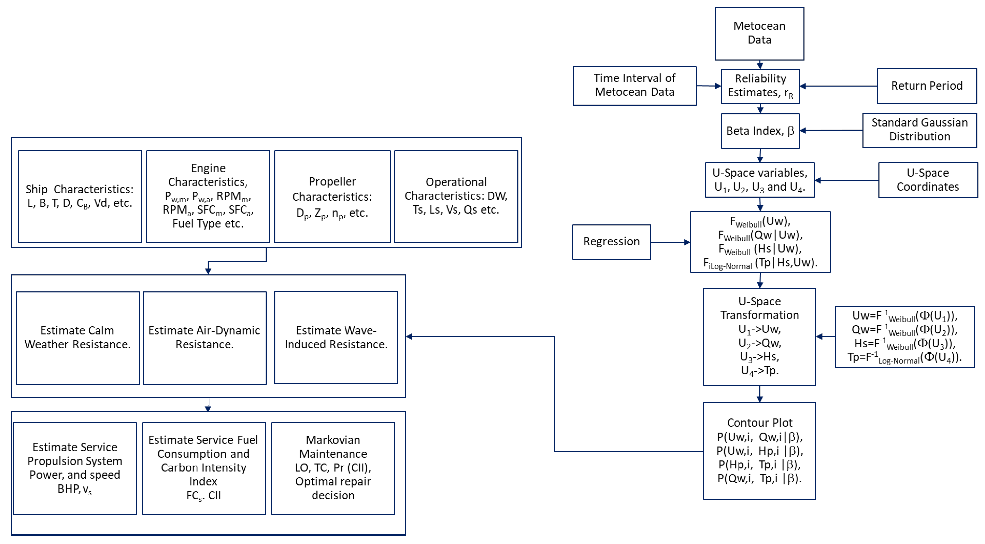
Figure 1 illustrates how the study’s framework makes use of both generated and pre-existing data. The information is organized into four main sections: (1) ocean data and analysis; (2) characteristics of the ship, engine, propeller, and operation; (3) calm weather, air-dynamic, and wave-induced resistance; (4) service propulsion system power and ship speed, fuel consumption, and CII; and (5) Markovian maintenance decision.
Section 2,
Section 3,
Section 4 and
Section 5 provide a thorough description of the four blocks. In
Section 2, the prediction of ship power is estimated, taking into account additional resistance in wind, waves, and calm waters. In
Section 3, the operating profile of the ship is examined to ascertain the propulsion system’s energy efficiency. The activity profile provides details about the ship’s intended course through the activity areas as well as the amount of time spent in each area. It also contains information regarding the tasks completed and the time given for each task. It also gives information on the average speed ranges of the vessel and how much time it spends at each speed in various wave heights and sea conditions. The strategies for maintaining the ship’s hull, thrust, and engine efficiency are covered in
Section 4. Finally, the ship’s propulsion system maintenance schedule is optimized in
Section 5 using a discrete-time Markov chain, taking into account both the current and future costs.
2. Ship Propulsion
For calculating the ship power prediction, including added resistance in wind and waves and calm water, methods with a minimum number of factors are considered to guarantee high accuracy, computational simplicity, and adaptability to a wide range of ship types.
While a ship’s performance is seldom tested in calm waters, it can vary significantly when operating in real sea states. However, ship design has primarily focused on designing ships for calm water conditions and additional resistance is then estimated using the ship’s experiences in various environments. The additional resistances brought on by wind and waves are also considered. Thus, the total resistance of the ship,
is determined as:
where
,
, and
relate to the calm water resistance, additional resistance in waves, and additional resistance due to wind, respectively. Manoeuvring and using the rudder wheel also increases the resistance. However, they tend to be less important and are therefore neglected in the present work.
Guldhammer–Harvald [
30], Holtrop–Mennen [
31], and Hollenbach [
32] methods are available for estimating the calm water resistance. Today, these widely used methods employ regression-based formulas that have been extensively tested in model research. The Holtrop–Mennen [
31] method has the largest applicable range and has fewer limitations, and it is used to calculate resistance in calm water in the present study.
To estimate the wave-induced resistance, ISO [
33] recommends STA-1 and STA-2 for all types of ships. STA-1 is limited to moderate sea conditions and STA-2 was developed to improve its applicability for higher sea states. Both STA-1 and STA-2 are only valid for head sea ±45 degrees to the bow, implicitly assuming that the additional resistance is zero for the remaining directions. Recently several methods [
34,
35,
36] have been proposed which perform significantly better and have the advantage of evaluating additional wave resistance on arbitrary wave heads. Since these methods require only a limited amount of information about the hull form, they are used when detailed ship hull information is not available. Therefore, the method proposed in [
35] is chosen here.
Wind resistance depends on wind speed, direction, and the area of the ship above the water line. The wind resistance has a substantial impact on the overall resistance of ships that have extensive volumes above the waterline. The estimation of additional wind resistance uses the methodology described in [
33]. This involves calculating the wind resistance coefficient through model tests or computational fluid dynamics simulations. Alternatively, coefficients can also be obtained from tabulated data based on previous tests conducted on similar hull shapes. In situations where wind tunnel tests or CFD calculations are not available, reliable estimates of wind resistance coefficients are provided in [
33,
37].
The total thrust efficiency is defined as
, where
is the hull efficiency,
is the open water efficiency,
is the relative rotative efficiency, and
is the ship hull efficiency [
38].
To evaluate the propeller efficiency in the initial design phase, the B-screw series [
39] is used. The series includes open fixed pitch propellers with blade area ratios from 0.30 to 1.05, pitch ratios from 0.5 to 1.4, and 3 to 7 blades. The open water characteristics of the Wageningen B-propeller series are described by polynomials derived from a regression analysis of the test results of 120 propeller models of the B-propeller series.
If the total resistance of the ship,
, efficiency of the propulsion unit,
and ship velocity,
are known, then the Brake Horsepower, BHP, can be calculated as follows:
The ship’s main engine is selected based on the propeller characteristics and overall ship hull resistance. The type of ship and operating mode are also used to determine the auxiliary engine profile. When the speed, required power, and technical data of the vessel are known, and the main and auxiliary engine power are defined including the fuel consumption, then the exhaust emissions of the vessel can be calculated.
Equation (2) defines the instantaneous power,
, as a function of the ship’s velocity [
40]. When the vessel is operating at its design speed, the maximum power,
, is typically 80% of the total installed main engine power, which is assumed to represent the engine’s Maximum Continuous Rating, MCR. When
, then the propelling power will be sufficient to move the ship at its design speed plus the safety margin.
Different ship types use their engines in diverse ways, particularly when visiting harbours; they may use different fuels both in and out of harbours. The type of ship determines the different requirements needed to generate electricity.
The auxiliary engines generate electricity during harbour stays and the main engines do not significantly contribute to harbour emissions during hotel stays.
The ageing of the propulsion system and fouling of the hull and propeller are reducing efficiency and need to be considered. The ageing of the engine,
, and fouling of the hull and propeller rates,
lead to an increase in the ship hull resistance as a function of time,
. The ship resistance, accounting for ageing and fouling is defined as:
where
is the elapsed time,
is the ship resistance at
= 0 (clean ship hull and propeller and maintained engine), and
and
are the latest times for engine maintenance and ship hull and propeller cleaning.
The ageing of the engine and the fouling of the ship hull and propeller will increase specific fuel consumption, as a function of time to satisfy the requested operational characteristics of the ship.
The simplest method, according to [
41] is to use the attained
to estimate each ship’s annual operational CII grates. Rather than performing in-depth computations of
emissions, this study uses the value of the total quantity contained in the EU MRV database [
42], yielding five CII rates: A, B, C, D, and E. Here, the probability that the maintenance will take place is also linked to the CII rates: unlikely (A and B), possible (C), likely (D), and certain (E).
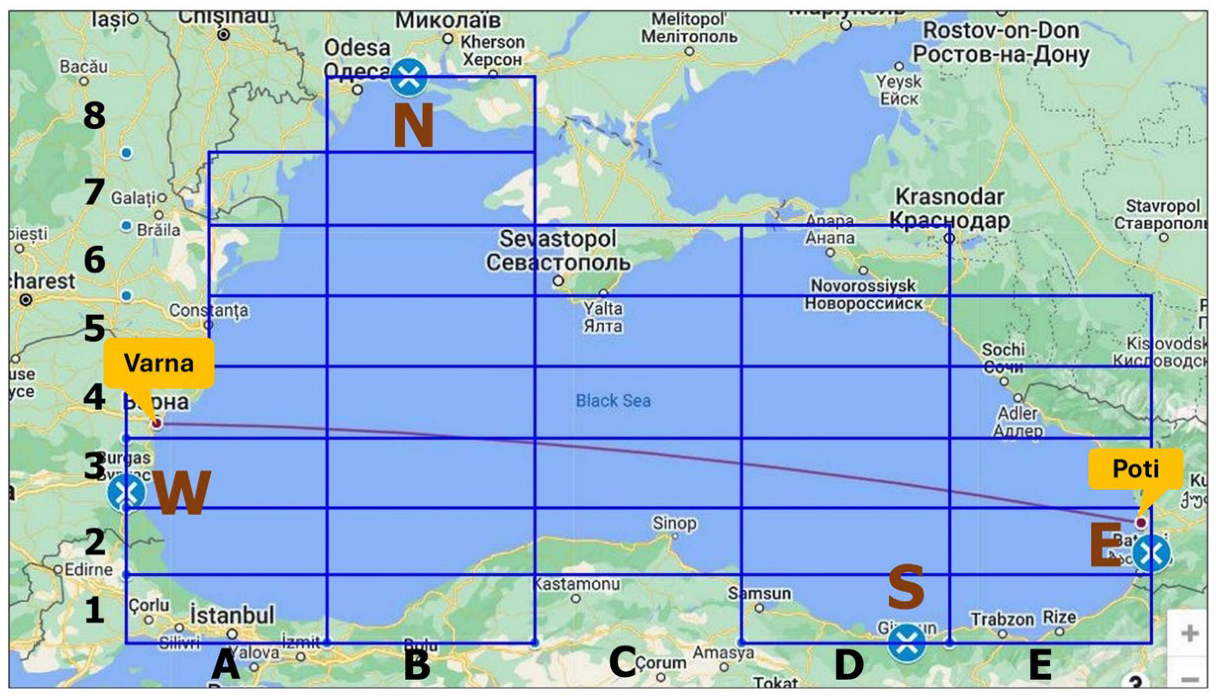
The main dimensions of the dry cargo ship used in the study are a length between the perpendicular of 181.7 m, a beam of 31 m, a depth of 16 m, a draft of 10.5 m, a block coefficient of 0.857, a ship design speed of 14 knots, and DW of 41,607 tonnes. The diameter of four-blade propellers is 6400 mm. The main engine is MAN 5G50ME-B9.5-TII (MAN Energy Solutions, Copenhagen, Denmark) with MCR 6650 KW × 97 rpm. The operational profile of the dry cargo ship operating between Varna and Poti of 658 nm, 93 voyages per year, leads to 61,200 nm travelled per year (
Figure 2).
3. Operational Profile
Detailed knowledge of a ship’s operating profile determines the energy efficiency of the propulsion system. The activity profile includes information about the planned route of the ship in the activity areas and the proportion of time devoted to each area. It also includes details about the tasks performed and the amount of time allocated to each task. Additionally, it provides data on the vessel’s average speed ranges and the amount of time spent at each speed in different sea states or wave heights.
This information can then be combined with a statistical representation of the wave climate for each region to produce a complete “ocean activity profile” for the ship.
Each parameter is discrete to perform calculations. To develop a detailed operational profile, it is necessary to input joint probability plots, including ship speed and sea state (or wave height). In developing the operational profile, speed and sea state are assumed to be independent. The next set of data needed is the distribution of time spent in each geographic area. The time spent in port should also be considered when designing a lifetime activity profile.
The Black Sea’s surface is divided into zones that cover specific geographic areas where the wave conditions are assumed to be uniform [
15] (see
Figure 2). These zones have approximate dimensions of 237 × 79 km (3:1) and are designed to accommodate the main traffic directions of S–N, S–N.E., and vice versa.
Information on significant wave height and wave period is obtained from the Copernicus Marine Service [
43]. Analysis and predictions for waves in the Black Sea are performed using the WAM Cycle 6, which is the third-generation spectral wave model. The model specific to the Black Sea operates on a spherical grid with a spatial resolution of about 2.5 km (1/40° × 1/40°) and consists of 24 directional and 30 frequency divisions. In total, there are 74,518 active grid points in the wave model.
The data has been collected over 20 years, starting on 1 January 2002 and ending on 31 December 2021. Observations were recorded every 3 h throughout the day.
The propulsion system is designed to operate in extreme environmental conditions. For example, if the BHP, generated CO
2, consumed fuel, ship speed, or attained CII are propulsion system control variables, then it can be considered that a random variable,
which represents the propulsion performance, is lower than specific thresholds,
with the probability of exceeding α mathematically. This condition may be defined as:
where
is the cumulative distribution function of the random variable.
The exceedance probability α corresponds to a particular recurrence, or a return period, which describes the average period between two successive states above the threshold
, called the return value at which the system operates, taking into account the random variable
, with a return period of
years [
44].
Offshore structures are monitored for overload failures in two limit states, the ultimate limit state ULS and the accident limit state ALS [
45]. ULS is associated with an annual probability of exceedance of 10
−2 and ALS with 10
−4. ULS is related to the design if the relationship between the load and the corresponding annual excess probability does not change rapidly. If so, ULS can be quite safe.
However, the nature of the load may vary, and significantly higher characteristic loads may be subjected to structures that are unlikely to be exceeded. Using a safety factor of 1.3, the calculated design load corresponds to an annual exceedance probability of approximately 10
−4 or less that meets the ALS requirement [
18].
With the modern design, all problematic load patterns associated with the load are identified with a 10−4 probability. However, in old structures where the load patterns have deteriorated, a misbehaving load mechanism may occur. Considering this, the probability of a misbehaving load mechanism should be considered, and an ALS system should be applied to environmental loads to ensure robustness against overload failures.
Using the applied load definitions in the case of a propulsion system that progressively is losing its efficiency, an annual probability of exceedance of 10−4 of the environmental condition is assigned to the analysis of BHP, generated CO2, consumed fuel, ship speed, or attained CII.
The safety operation of a ship’s propulsion system depends on the existence of many variables,
, and their correlations. A joint probability density function of those variables can be defined. In the present study the significant wave height, spectral peak period, wind speed, wind direction, and ship heads are considered. An environmental contour [
18] is constructed that covers a subset of the environmental and operational conditions under which the propulsion system is intended to operate, and this area is defined as the design region. The most critical propulsion system responses are associated with extremely high or low levels of any range of environmental and operational variables, i.e., environmental conditions at the edge of the design range.
Propulsion system behaviour is analysed regarding limited environmental and operational conditions along the contour rather than combining several possible variables across the design domain [
44]. When more than two variables are involved, the environmental contours lead to surfaces for three or manifolds for more than three variables.
The traditional and most used approach of the Inverse First-Order Reliability Method (IFORM) [
18], which became a design practice for ocean engineering applications such as ships, offshore structures, or wave energy converters, is employed here.
The Inverse First Order Reliability Method (IFORM) first defines the contour in the normal space, instead of the original environment variable space, , where the radius of the 2-D or n-D surface is defined, and the radius corresponds to the return period and increases as the period increases. The points of the U-contour are transformed to the original variable state, resulting in the X-contour.
The transformations are performed with Rosenblatt’s inverse transformation [
46]. IFORM is a reliability method that uses the idea that the exceedance region defines the failure area (and exceedance probability
α) and approximates the probability of threshold level crossing of the propulsion system control variables [
47]. Nowadays, IFORM-based contours are widely used in different industries [
19,
48,
49,
50,
51,
52,
53,
54].
This study analyses 600 environmental conditions that correspond to an annual exceedance probability of 10−4 that meets the ALS requirement and estimates the BHP, CO2 emission, fuel consumption, ship speed, and CII generated by the propulsion system during sea operation in the route Varna-Poti-Varna.
For convenience, the wind speed,
, and direction,
, significant wave height,
, and wave period,
are defined as
and are considered random variables in the space
. The joint probability distributions of
are available as the marginal distribution of
and the conditional distributions of
given
, and
given
and
given
and
. The most precise estimate of the generated
is derived from the return period of
years and the probability of occurrence of the average values of the random parameters
, representing these variables as conditional median values. The model was developed to estimate carbon dioxide based on a return period that includes the uncertainty of all significant environmental variables called a “4-D” probabilistic model based on the measurement interval,
, and variables
, where the Beta index β is defined as:
The recurrence period
is calculated as:
where
is the annual occurrences of the random variables. Each combination of
on the 4-D hypersphere is then transformed into physical joint random variable space and defines combinations of the physical random variables (
,
,
, and
) with
= 3 h,
, and
= 3.72.
The inverse reliability procedure like the IFORM [
18] is less computationally intensive and has an essential advantage in that it offers valuable insights into the derived BHP, generated CO
2, consumed fuel, ship speed, and attained CII, conditional to the associated environmental conditions.
It describes a -dimensional hypersphere, specifically with , for variables . The hypersphere has a radius equal to the target Beta index, , which represents independent standard normal variables. Each of these variables pertains to a physical random variable. At any given point on the hypersphere, it is possible to draw a tangent hyperplane. This hyperplane represents the probability of the points occurring on the side of the hyperplane that is furthest from the origin. This probability is defined as , and is calculated using a local linearization method of the serviceability limit state function at the design point. In this context, refers to the Gaussian distribution function.
Since each point on the hypersphere in the U-space is associated with the same reliability level when estimating
, the points on the hypersphere in the X-space can be systematically checked until the most significant derived BHP, generated CO
2, consumed fuel, ship speed, and attained CII is encountered. The conversion from the standard normal distribution in the U-space to a physical random variable in the X-space is made using the Rosenblatt transformation [
46].
The design variable
, may be determined if the cumulative distribution functions,
,
,
, and
, and the target beta index
are known as:
For each value of
the quantile value
is calculated using the inverse standard Gaussian distribution:
where
and
The environment of the shipping route is analysed, where 3-h joint environmental statistics of
(10 m above the mean sea level),
,
and
are collected specifically for the present study, where the joint probability distribution is defined as:
The Weibull distribution is assumed to follow the marginal probability distributions for
,
, and
parameters, while the Long normal distribution is assumed for the
parameter. The extreme value distributions were fitted satisfactorily for all four parameters to the marginal data. The wind speed follows the Weibull distribution:
where
and
are estimated as 1.81 and 4.14, respectively.
The conditional distribution of turbulence, given the wind speed, is assumed as a log-normal distribution, where the mean value and variance are a function of wind speed:
where
and
The conditional wind direction also follows the Weibull distribution:
where
where
,
,
,
,
and
are estimated as 0.5, 1.18, −0.66, −2760.57, 22,929.96 and −0.02, respectively.
The conditional significant wave height also follows the Weibull distribution:
where the dependence of model parameters as a function of the wind speed is modelled with different power law relationships as
where
,
,
,
,
and
are estimated as −61.32, 62.81, 0, 1.13, 0, 3.89, respectively.
The spectral peak period conforms to the log-normal distribution, given a combination of
and
:
where
where
,
,
,
,
and
are estimated as 1.62, 2.31, 0.55, 0.38, −0.22 and 0.29, respectively.
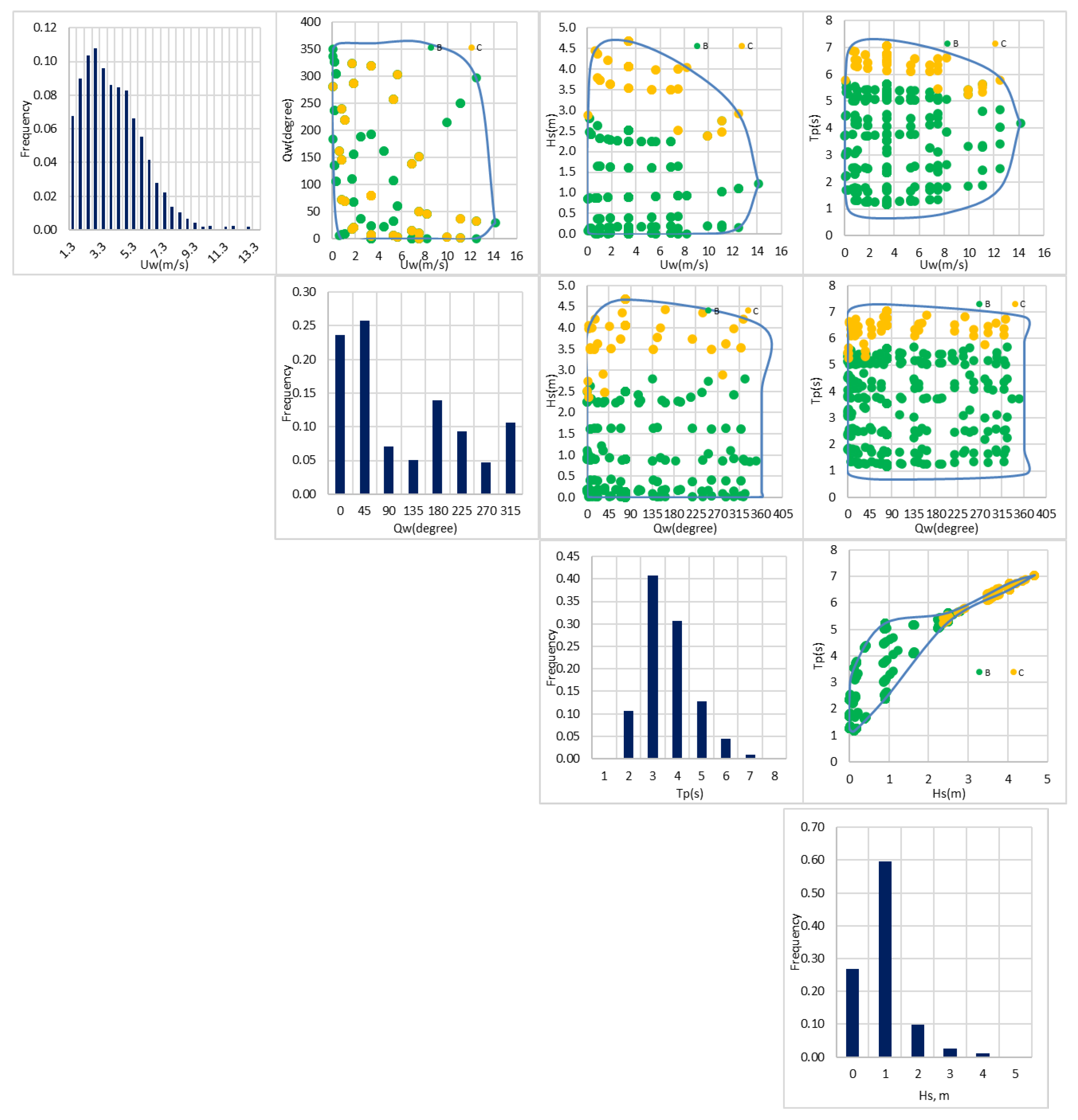
The histograms and contours of the wind speed, direction, significant wave height, wave period, and distribution of CII for LE(0) are shown in
Figure 3.
5. Markov Decision Processes
To model changes in the rate of CII over the years using a Markov chain [
64] and a set of states
are defined and the probability mass function for the initial configuration is identified. A conditional probability mass function that describes the transitions between these states is established. The probability mass function can be expressed as follows:
which expresses the absolute probability of being in state
at the time
or in state
after
transitions. For the special case when
, the value of
represents the probability of starting in state
. If there are
states
, the initial probability vector
can be expressed in an
-dimensional form. This can be done by following these steps:
The conditional probability mass function is defined as:
where
indicates the probability of being in state
at the time
if it is in state
j at the time
. If the string is stationary, the notation is
. If
= 1, it is a one-step transition probability.
The transition matrices are used in simulating the gradual transition of CII employing the Markov transition probabilistic model. All ship CII rates belong to one of five different CII intervals or states that form the basis of the Markov transition probability model. The probability matrix indicates the possibility that the CII rate remains constant or moves to another class in a given time horizon and can be used to construct a transition matrix for discrete cases in which all estimated CII can be organized. Each matrix entry indicates the probability that the CII is equal to at the time and j at the time .
The elements of the transition matrix have the following properties:
The present study analyses 600 environmental conditions that correspond to an annual exceedance probability of 10−4 and estimates the BHP, CO2 emission, fuel consumption, ship speed, and CII generated by the propulsion system of a dry cargo during sea operation in the route Varna-Poti-Varna.
In this respect, evaluating the Markov transition matrix is a straightforward process once the states of each transition are defined. The probability of changing the CII rate of the dry cargo ship in several operational conditions can be determined if their rates are known at the beginning of the state (year) and again at the beginning of the next state (year). The probability that the ship in several operational conditions,
, have a certain CII rate
in period
and CII rate
in the period
can be estimated concerning the total number of operational conditions that the ship encounters in the year
to the number of operational conditions the ship encounter at the same CII rate in the year
. If
represents the set of operational conditions in state
in period
and in state
in period
, the components of the transition matrix for multiple operational conditions must also satisfy the following conditions when information is limited about the transition between various operational conditions [
28].
and
is estimated as:
The probability of transition of a number of the operational conditions encountered by the dry cargo ship whose CII rate started in state and ended in state j divided by the total number of the operational conditions that the ship encounters that started in state gives the probability of transition from any state . The estimate given in Equation (16) is the maximum likelihood, which is consistent, but it is biased, and the bias tends to zero as the sample size increases.
The probability of transitioning from the state to the state j for a dry cargo ship, divided by the total number of operational conditions that started in state gives the probability of transitioning from any state Equation (16) provides an estimate of this probability, known as the maximum likelihood, which is consistent but biased. As the sample size increases, the bias tends to zero.
By analysing the chain after
transitions, one can calculate the accumulated probability for all transition segments that end after
n transitions. The information about the state after
n transitions is stored in an unconditional probability vector
which is computed as:
For each state of the Markov chain, a decision is made about which alternative maintenance actions should be taken in that state. The chosen course of action will affect the transition probabilities and costs associated with additional fuel, maintenance, and lost opportunities over the life of the ship’s propulsion system. Optimal maintenance is determined by considering both immediate and subsequent costs, and the decision process is related to a Markov decision process [
20].
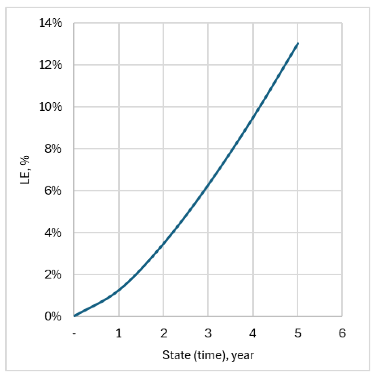
Ship hull, propeller, and engines are of permanent service, and due to that, the ship hull and propeller are fouled, and the engine deteriorates with time in both quality and power output. Therefore, at the end of a specific period, an inspection is done that results in classifying the deteriorated condition into one of five possible states, which are related to loss of efficiency, LE defined as LE(0) = 0.0%, LE(1) = 1.24%, LE(2) = 3.47%, LE(3) = 6.29%, LE(4) = 9.52%, and LE(5) = 13.04%.
After simulating the operational behaviour of the ship in specific open sea conditions, accounting for the generated CO
2, data on deterioration conditions and the CII grates are gathered, and statistical analysis is performed identifying the state of the complex ship hull-propeller-engine transits from state to state. The matrix in
Table 1 shows the probability of each transition from the CII grades A, B, C, D, and E from the LE(0)-state to the LE (1)-state.
In addition to the statistical analysis, it is found that the transition probabilities are unaffected by what the states were in the prior status. This “lack-of-memory property” is associated with the Markovian property. Therefore, the random variable of the attained CII grate, which is the state of the ship-propeller-engine at the end of the state, is a stochastic process associated with a discrete-time Markov chain whose one-step transition matrix is shown in
Table 3.
An alternative to recover the system to its previous or original state is to perform maintenance and repair. This option does not improve the propulsion system while in states A or B, so it is of interest only in states C, D, and E, and the last one coincides with the non-operational state. In this state, a renovation would return the system to state A or B. However, this will involve consequences in loss of profit from the loss of opportunity, LOC. The total cost, TC of any maintenance decision included the annual additional fuel cost, AFC, maintenance cost, RC, and loss of opportunity cost, LOC as defined in
Table 4.
Following the progressive degradation of the propulsion system, and once the maintenance is performed, the system is returned to state A or B, representing a new state. The model for the Markov decision processes is defined as the state of the discrete-time Markov chain is observed after each transition, , where after each state identification, a decision is chosen from a set of possible decisions, where . If decision is made in the state , an immediate cost is accumulated that has an expected value of . The decision in the state determines what the transition probabilities will be for the next transition from state with transition probabilities by for . A set of decisions for each state, known as , determines the policy for the Markov decision process.
The objective is to find an optimal policy according to some cost or operational criterion (CII grates, fuel consumption, CO2 generated, ship speed reduction, and required engine power) which considers both immediate and subsequent costs that result from the progressively lost efficiency of the ship propulsion system.
The Markov chain represents the state of the ship’s propulsion system, and after each inspection, a choice is made between five maintenance decisions according to
Table 4. The new transition probabilities depend only on the current state and the maintenance decision, and the instantaneous expected costs also depend only on the current state and the maintenance decision.
The maintenance strategy is deterministic, meaning that when the system is in state I, the decision rule selects only one maintenance option. The maintenance decision rule is always the same, regardless of the system’s current state. In doing so,
, where the initial maintenance decisions made in the state
assumed here are gradually increasing as the CII grates progress, and
denote a specific policy.
Table 4 shows the total cost consequences associated with the recovery to the initial CII grates, which are associated with do nothing for A, minor for B, moderate for C, major for D, and extreme for E, respectively.
The (long-run) expected average cost per unit of time
then can be estimated as:
where
) for each state and
represents the steady-state distribution of the state of the propulsion system under the maintenance policy being evaluated.
It is also assumed that the evaluated ship propulsion states are also associated with the time following the exponential relationship, (see
Figure 4):
The incremental growth of BHP, AFC, generated CO
2, and the ship service speed,
, in absolute value and CII rates in
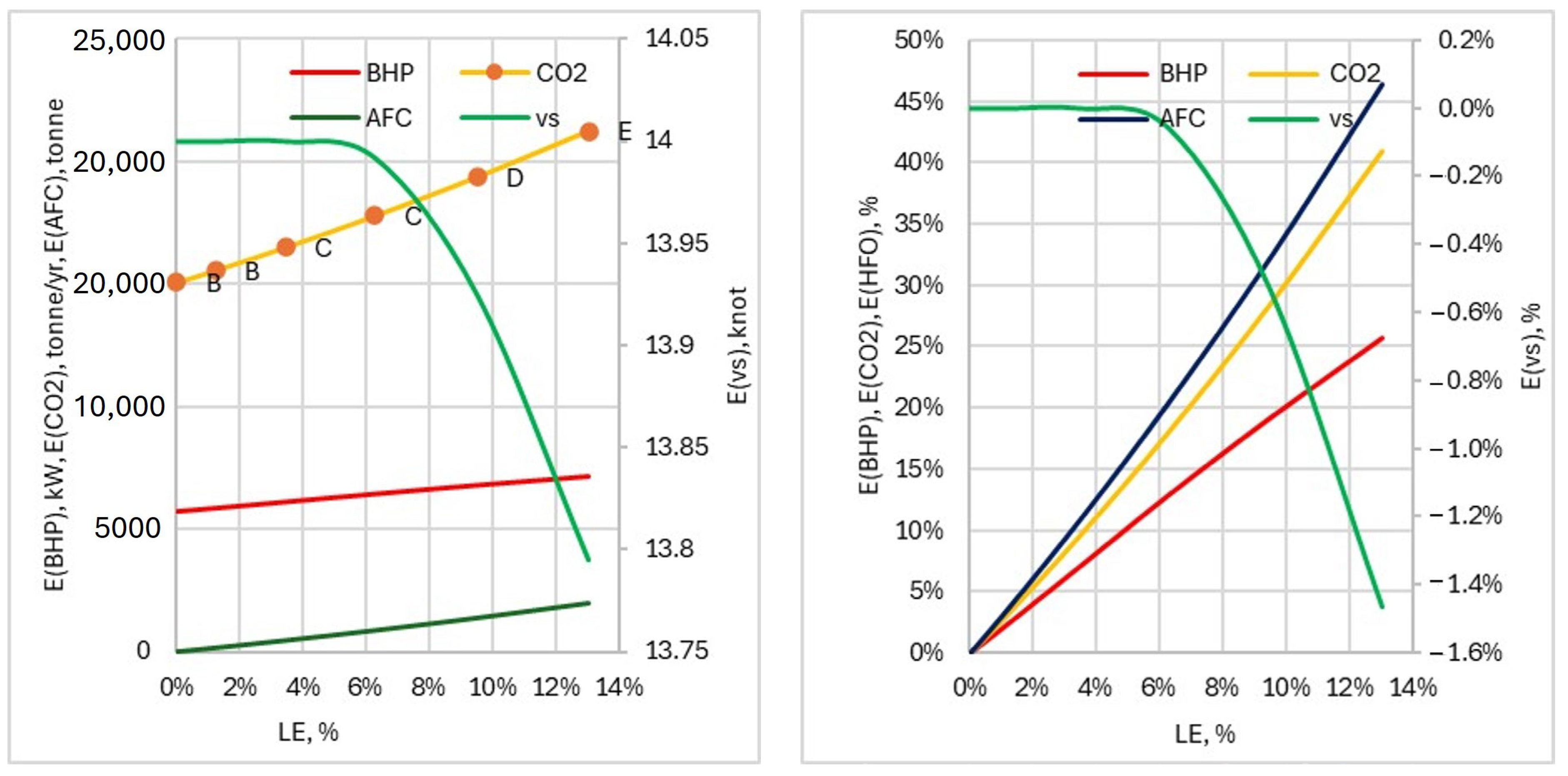
Figure 5 (left) and per cent concerning the initial zero state is given in
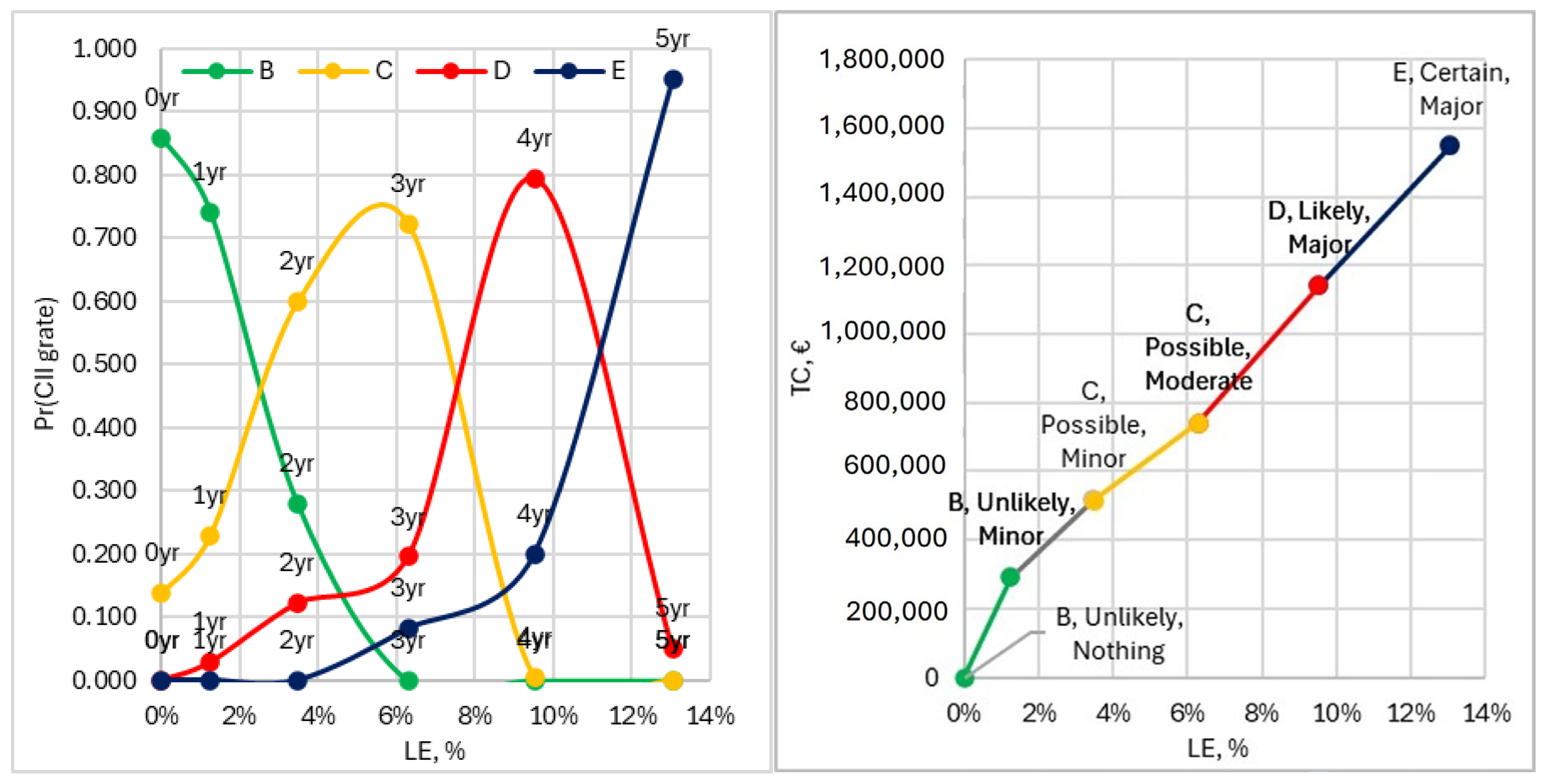
Figure 5 (right). The resulting probability of the CII grates as the degradation propagates with progressive loss of efficiency is shown in
Figure 6 (left) and the (long-run) expected average cost is in
Figure 6 (right).
Additionally,
Figure 6 (right) illustrates the likelihood that the maintenance will occur (unlikely, possible, likely, and certain), as well as the estimated depth of the maintenance and its financial implications (nothing, minor, moderate, and major).
An algorithm is implemented to improve the initially assumed maintenance policy. A series of equations are employed to find
and
in identifying an optimal maintenance strategy. For any maintenance policy
, related to the respective transition probability defined by the Markov transition matrix for any state,
, and the total cost associated with any
th state and
th decision,
, a series of equations can be defined as:
Using the cost of
computed for the maintenance policy
, an alternative policy
is defined such that, for each state
, where
minimizes:
and then
, set to the minimum value of
k, defines the optimized policy
for all identified optimal solutions,
. For the current study, the optimal decisions are indicated in
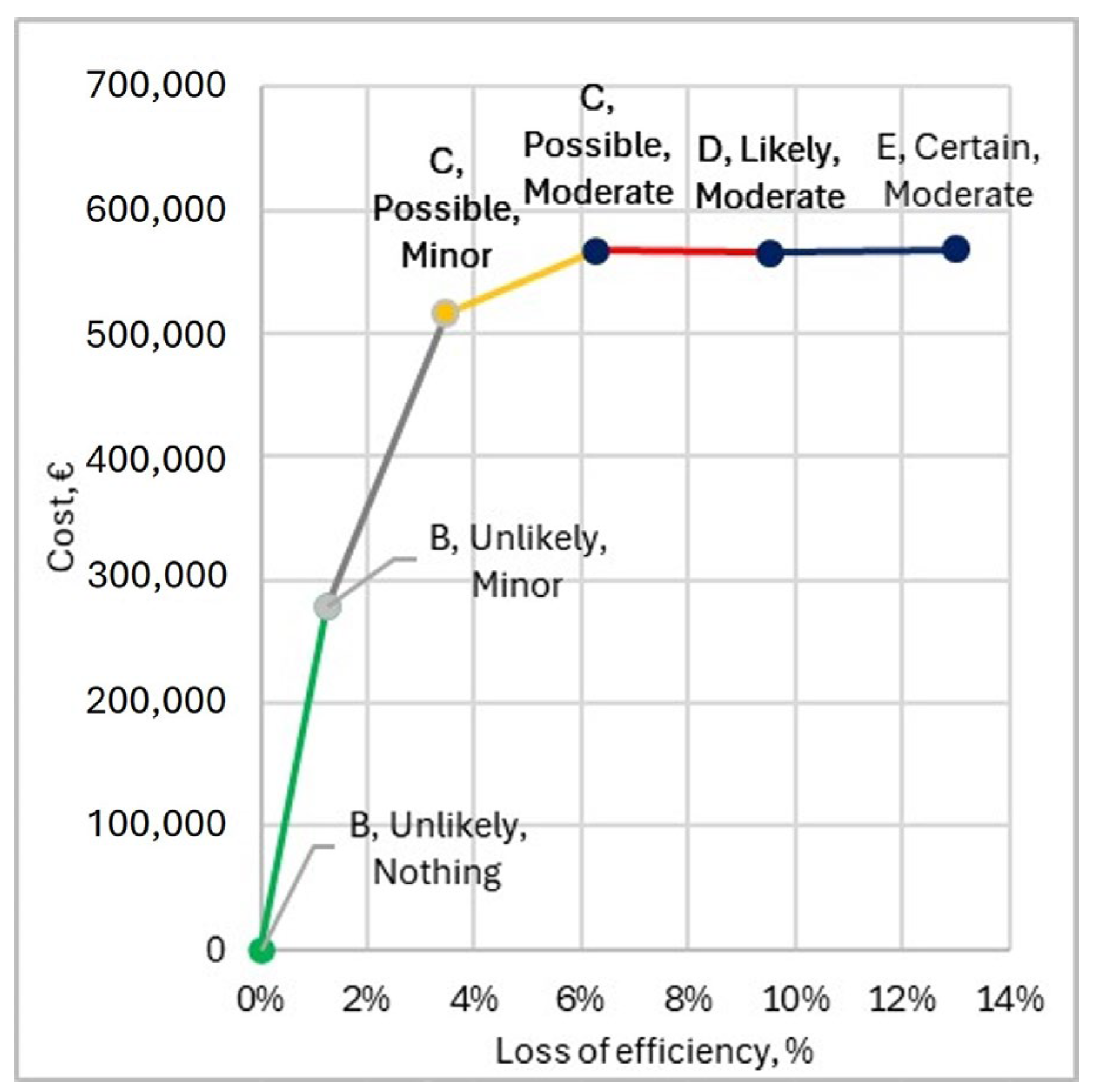
Figure 7.
Therefore, there is a difference between the optimal maintenance policy and the initial assumption. Lastly,
Figure 7 illustrates the cost related to the best maintenance strategy. It is apparent that the CII is maintained, as is the possibility of maintenance; however, the maintenance from the major level decreases to moderate, and the associated costs are also decreased.
Employing an optimisation algorithm improves the initially assumed conservative maintenance policy to the optimal maintenance decision for each level of degradation, for the initially defined environmental and operational characteristics of a dry cargo propulsion system while considering both the present and future costs.
The approach presented focuses on how to optimally design a discrete-time Markov chain ship propulsion system maintenance through a choice regarding which of multiple actions should be made at each potential state of the Markov chain. The decision made has an impact on both the upfront costs (or benefits) and ongoing system operating expenses.
