1. Introduction
This research is motivated by the notable commitment of society, companies, and enterprises to reducing energy consumption when performing operations by industrial robots. According to recently published reviews, articles, and papers, a decrease in energy demand not only contributes to the economical use of natural resources, but also boosts robot lifespan and manufacturing sustainability.
This comprehensive review [
1] lists the main resources involved in energy saving, including cost-effective equipment and programming technologies. It is shown that the selection of efficient motors, drives, and controllers can significantly reduce energy demands. Along with hardware improvements, many novel programming technologies exist that help to exclude unnecessary robot motions and joint reorientations, optimise travel routes, and apply smart velocity profiles with minimal accelerations and jerks. By improving robot programs and operation schedules, many processes may be accelerated to minimize the energy consumption of industrial robots. In article [
2], a detailed evaluation of robot energy needs is presented for different operations and execution cycles, and the optimal work schedule is derived as a solution to the mixed-integer nonlinear programming problem. Study [
3] describes a new approach to robot path planning. This enables the minimisation of energy consumption, wherein care is taken regarding the persistence of critical mechanical components during the robot cooperation with mobile platforms. The authors of [
4] propose a simulation method for generating low-energy motions using quantum computing technology. The problem is formulated as a search for the transitions of robot positions in terms of workspace and work time, using the total torque required for the motion as an objective function. In [
5], a trajectory planning method with minimal energy consumption is offered based on an improved sparrow search algorithm. In paper [
6], an optimization procedure predicts a decrease of up to 30% in energy and up to 60% in peak power for the trajectories, using various cost functions and examining the algorithm for a variety of scenarios. In [
7], energy-optimal trajectory planning and initial pick point searching problems are studied for palletizing robots with high load capacity and high speed, in which both the pick point and the place point are fixed to a desired location for each single task. The performance indexes are given within for the rigid–flexible coupling dynamics and the boundary conditions of the robot. The fourth-order Runge–Kutta method, multiple shooting method, and traversing method are used to solve these specific mathematical problems. Article [
8] focuses on trajectory optimization, whereby the detailed collision detection of individual robots is included in the analysis. It is demonstrated that energy optimization for cramped robot cells is possible, and that efficiency losses are insignificant compared to optimization results without it. In [
9], a method is presented for the optimization of trajectories in robots with six degrees of freedom (DOF) and a spherical wrist. Additionally, the maximization of manipulability and the minimization of electrical energy take place in a way that considers the kinematics and dynamics of the manipulator in order to integrate an algorithm based on the Kalman method for calculation purposes.
Robots with parallel and serial topologies compete in the modern market in terms of numerous technical indicators. In a number of applications, the parallel robots have prominent advantages over their serial counterparts, such as a greater payload capacity, fewer positioning errors, higher rigidity, less inertia, and better dynamic characteristics that are suited to the rapid manipulation of processed parts [
10,
11]. This applies in particular to the pick-and-place (PnP) processes, in which the parallel-type linear Delta robots (LDRs) have specific benefits thanks to their better ability to withstand inertial overloads, along with accurate and fast movement. These features of the LDRs are even more important issues for energy optimization than in the case of serial machines, despite their limited DOF [
12,
13].
Various model-based control principles are used to LDR manage, develop, and study [
14,
15,
16,
17]. Unfortunately, due to design complexity, most of their physics–mathematical models are designed for solving either kinematic, statical, or dynamics-related problems separately, and do not have sufficient completeness to optimize energy consumption. Hence, new computer models are required for supporting the simultaneous resolution of both the forward and inverse kinematic (for route optimization), statical (for power optimization), and dynamics-related (for energy optimization) issues of robotics.
In this regard, it is useful to address neural network (NN) technology that enables the successful adoption of new inputs and the performance of human-like intelligent tasks, such as reasoning, making decisions, or solving problems. Among the recent studies related to machine learning in robotics, some studies may be strengthened, such as [
18,
19,
20,
21,
22]. In a review on NN developments initiated in [
23], a comprehensive study of multiple research articles published from 2014 is presented, considering the domains of industrial informatics. Based on these publications, it is appropriate to infer that the main advantages of all NNs are their learning ability, fault tolerance, and real-time operation, possibility resulting from their high computational speeds. They can be trained to classify data, recognize patterns, and detect sequential dependencies in the inputs. To employ these benefits, various single- and multilayer, feedforward (forward propagation), and recurrent (backward propagation) NNs are developed, including deep NNs with many hidden layers, convolutional NNs suitable for image, and audio and text processing.
In the current study, the multilayer feedforward fitting NN capable of forecasting future events was selected. This, in contrast to other topologies, provides extensive opportunities for learning from the preliminary measurements performed on real machines. Thanks to its purely data-driven nature, this NN does not require complete knowledge of all the geometric and mass properties of the robot and its environment. Additionally, the fitting NN models are suitable for adaptation to the changes in robot architecture occurring over time in line with regular industry updates.
In this article, solutions to two research problems are reported based on the fitting NN models considered. Both of them focus on energy saving in PnP operations, without any investments in hardware, based on the selection of the best robot joint configuration (JK), i.e., a set of locations that robot joints may take while placing the tool in a target position [
24,
25].
The first way to save energy concerns the minimization of the robot power consumed in a separate tool position (target). The goal is to find the JK for each target that requires a minimal supply power in terms of statics. This problem is real for processes such as quality control, welding, packaging, or wrapping, in which the steady-state placing and holding phases of the PnP cycle continue for much more time compared with picking.
An objective function of the second problem concerns the minimum total joint route distance through all targets, considering all possible JKs at which the overall energy consumption becomes minimal as a result of reducing the duration of the PnP process. This solution is actually used for the systems that require the fastest picking and placing cycles with relatively stable power consumption, such as assembling, loading, or painting.
To solve the above-stated problems, the new NN-based models of the LDR are developed in line with a novel consumed-power monitoring procedure, which aligns detailed power estimation at different JKs with joint route optimization to reduce the energy demand.
Both solutions are supported by simulation procedures based on MATLAB R2023b libraries and apps; these are constrained by the possible locations of the tool, processed parts, trajectories, joint properties, arm dimensions, mass, inertia, and velocity profiles. The feasibility and applicability of the offered optimization tools are confirmed by measurements of the real Festo EXPT-45-E1 robot.
The contents of this paper are arranged as follows. First, the mathematical formulation of the problem is given, and the NN-based computer models design of the LDR is presented. Next, a search procedure for the JKs with the lowest power demand is described. Then, a technique is established for planning the shortest route that the joints can pass between given the initial picking and final placement positions in the total PnP process, following which the robot consumes the lowest energy. Finally, the experimental results are evaluated, and conclusions are drawn.
2. The Problem Statement
The joint dynamics of the LDR are described by the Newton–Euler equation [
26]:
where
is the joint torque applied to
th joint;
is the fraction directed at overcoming external disturbances;
is joint stiffness, dependent on the internal body mass resistance;
is the damping factor;
is the moment of inertia; whereas
represent the vectors of joint positions, velocities, and accelerations.
The electromagnetic fraction of torque generated by an electric motor with flux linkage
and supply current
is given as:
At given supply voltage
, this yields the electrical power required to keep the joint:
The energy consumed during the PnP cycle of the time length
t is given as follows:
According to (1), the torque developed by the joint motor is composed of two parts, namely, the holding torque needed to withstand constant external and internal influences, and the moving torque required to move, accelerate, and decelerate the arm due to robot inertia. Therefore, the current study considers two research problems, and two different solutions are found. In the first case, the focus is on the retention of the processed part in the target position, and the problem is reduced to solving (1) for only. In the second case, the total electricity consumption of the moving LDR is the focus.
When looking for solutions, it should be borne in mind that the total power
and energy
consumed by the
-DOF robot are determined not only by the common joint power and energy, but also by the additional parts
and
associated with system losses in motors and gears, power converter, fans, sensors, control equipment, and other needs of the robot system. This is given as follows:
This means, the electricity consumption of the robot depends on both the JK and other factors, and it is quite a complex problem to assess the ratio of system and joint power and energy components. In this research, this ratio is sought experimentally.
Once the consumed power and energy (5) are found, the objective function of the research is represented:
3. Materials and Methods
The described approach addresses a 3-DOF LDR, shown in
Figure 1. The robot contains a triangular fixed-base platform, three identical arms, and a mobile tool flange. Each arm consists of a couple of parts, namely, the upper motor-driven linear rail joint, such as A1, A2, or A3, which has a toothed belt gear, and the lower parallelogram rod, connected at one end to the rail by a passive joint and at the other end to the tool flange by another passive joint. These spherical joints drag the tool flange along the Cartesian XY frame, parallel to the base platform, and vertically along the Z axis.
The robot dimensions are presented in
Table 1 [
27].
Due to many unknown, non-linear, and unstable factors in (5), most of the conventional physics–mathematical models of LDRs cannot jointly solve forward and inverse kinematics problems on the one hand and static problems on the other hand, whereas it is the latter that are needed to minimize consumed power and energy (5), (6). Unlike kinematics, robot behavior in statics depends on the mass of the processed object, its shape, and the way it is gripped, and all these factors affect energy consumption. For this reason, the focus of attention has been shifted to NN models suitable for solving complex problems and capable of providing higher efficiency, cost savings, and accuracy compared to physics–mathematical solutions.
The first and most important step in the development of any NN model is related to the collection of the sufficient quantity of data required. In the condition when complete open data sources of the LDR are absent, the measurements of the real robot are to be performed with the foremost aim of composing an NN capable of predicting the power and energy demands in various kinematic configurations. The conventional relational tabular database was chosen as the source for further NN training and testing.
Many data collection methods have been proposed for 3D workspace estimation without emphasis on energy consumption, such as in [
28], where the workspace is divided into a regular voxel grid; in [
29], where the 3D space is segmented into a pillar grid; or [
30], where the features are directly extracted from raw point clouds. In the current data accumulation procedure, three LDR linear joints—A1, A2 and A3—were conditionally divided into rail segments, one after the other. Based on the lengths of the linear rails given in
Table 1, the volume of the dataset was set as
m = 496 tool positions (tabular rows), with 7 parameters (tabular columns A1, A2, A3, X, Y, Z, and P) each. During the systematic moving of the joints along these segments with a 24.6 mm step, joint coordinates A1, A2, and A3 and Cartesian tool coordinates X, Y, and Z were read with the help of the Festo CDSA-D1-VX teaching pendant. These coordinates are determined by the LDR geometry and do not depend on robot physics (mass, inertia, friction, stiffness, damping, etc.).
To estimate consumed power, a Fluke 1745 power quality logger with PQ Log 2.2 software granted by Fluke was applied. Since these data are defined by LDR physics, they reflect the particular mass of the processed object, its shape, and the way it is gripped.
Given that all collected data initially have the required format, they can be sent directly to the NN designer without complex preprocessing.
Next, using the MATLAB R2023b NN Fitting app (
nftool) [
31], the model was designed in the form of a tandem of multilayer feedforward NNs. The first NN is intended for simultaneously solving the forward kinematics and power consumption (FKP) problems. To compose it, all accumulated observations were regrouped into two arrays and imported in the NN Fitting app as an {
m to 3}-size array of predictors A1, A2, A3 and an {
m to 4}-size array of responses X, Y, Z, and P. The second NN is intended for simultaneously solving inverse kinematics and power consumption (IKP) problems. To compose it, the same observations were imported in the NN Fitting app, but in this instance the {
m to 3}-size array of predictors consisted of X, Y, and Z data, whereas an {
m to 4}-size array of responses consists of A1, A2, A3, and P data.
In both cases, imported data are distributed between the training set for learning (70%), the validation set for NN verification and the prevention of overfitting (20%), and the test set for independent checking (10%).
The synthesis of a NN begins with a simple double-layer feedforward topology with a few hidden neurons, a sigmoid transfer function in the hidden layer, and a linear transfer function in the output layer. Three training algorithms, namely, the fast Lavenberg–Marquardt algorithm, the slow but accurate Bayesian Regularization algorithm, and the memory-efficient Scaled Conjugate Gradient algorithm, were compared to the {
m to 3}-size array of predictors and {
m to 4}-size array of responses upon random data division, an initial layer size of 10, and a maximal number of epochs of 1000. Training results were qualified by the number of epochs that passed before stopping, the mean square error (MSE) performance, and regression (R). The average results of this comparison are collected in
Table 2.
The Bayesian Regularization algorithm was selected for further NN training due to its achievement of the best MSE and R indicators. During the NN training, its structure was optimized by changing the number of neurons and activation functions in hidden layers to improve the model’s quality. The following results were obtained: MSE = 0.00715 and regression R = 0.9986 in training, MSE = 0.000012 and R = 0.9983 in validation, and MSE = 0.00036 and R = 0.9972 in testing.
After training, the NN codes generated by the app were forwarded to MATLAB for their use as the LDR models suitable for finding the subsequent solutions of the FKP problem and the IKP problem, appropriately.
4. Results and Discussion
4.1. Using the NN as an FKP Solver
To validate the developed robot model as an FKP solver, the following procedure is performed. First, an {s to 3}-size joint array (JOINT) is generated, where s is the number of permissible A1, A2, and A3 joint positions, where s >> m. Using the NN model, this array is transformed into another {s to 4}-size array, with Cartesian tool coordinates of X, Y, and Z and consumed power, P (CARTP). A small part of the JOINT and CARTP arrays are consistent with the data obtained earlier, while most of them are intended for use in predicting possible LDR states and behavior.
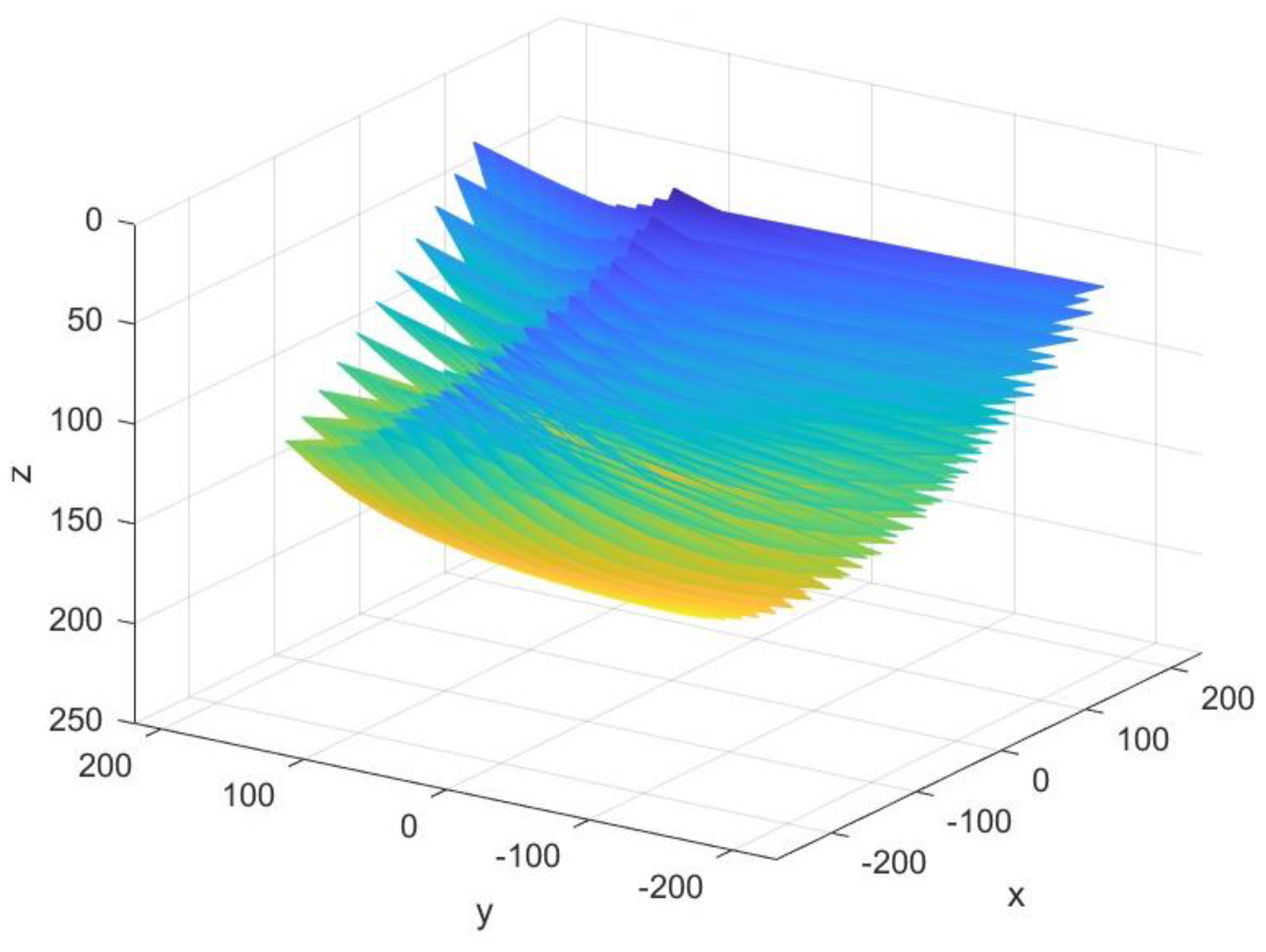
The obtained CARTP array is suitable for estimating the robot 3D workspace, i.e., a set of all spatial positions that a tool might reach without collisions and singularities. To identify the workspace, the forward kinematics problem is solved repeatedly, while every joint cyclically increases its position value within the prescribed limits and Cartesian tool coordinates are saved. The robot workspace plotted with the help of the designed FKP solver is displayed in
Figure 2, where Cartesian tool coordinates X, Y, and Z are measured in millimeters.
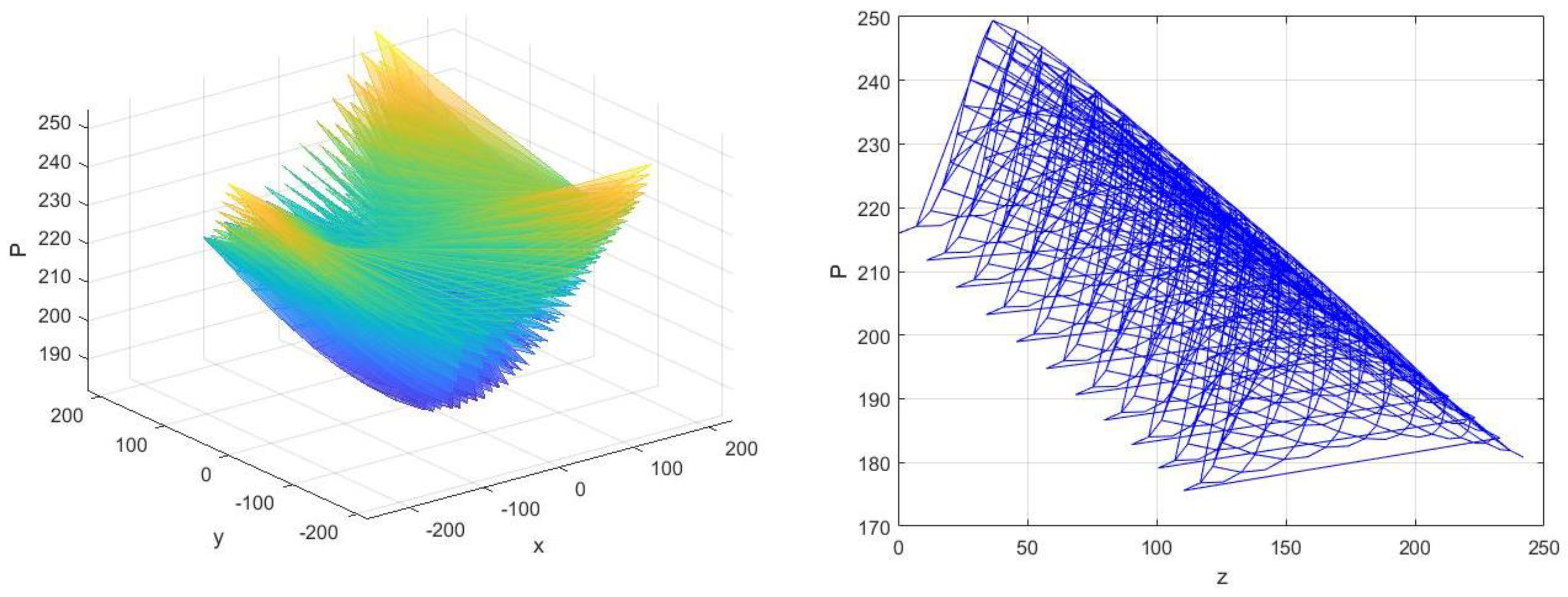
Figure 3 demonstrates two non-linear dependences of the power consumed by the robot on Cartesian coordinates, plotted with the help of the FKP solver designed, where Cartesian tool coordinates X, Y, and Z are measured in millimeters and consumed power, P, is measured in watts. These diagrams show that minimal power is consumed when the tool is lifted above the central part of the work plane. The farther the tool moves away from the center and the lower it descends the greater the power that is consumed.
4.2. Search for the JKs with the Lowest Power Demand
Considering that LDR accuracy must always exceed the tolerance of PnP operations a robot performs, every joint location in the JOINT array may result in a number of similar Cartesian locations in the CARTP array. This means that different power amounts can be consumed while the tool achieves the same Cartesian positions at different JKs. Consequently, a search for the JKs with the lowest power demand may be chosen as a key factor in the optimization procedure in the steady state.
The proposed method for searching the best JKs tends towards the common solution of the inverse kinematics problem. In [
32], various algorithms known in robotics are compared to generate solutions to inverse kinematics problems. Usually, they employ iterative gradient-based optimization approaches that start with an initial guess about the solution and seek to reduce a specific cost function. Since most of them fail with some combinations of the initial assumption and target tool positions, not all inverse kinematics and power estimation requirements can be met with their help. This is especially important for the LDRs that are the 3-DOF machines of parallel architecture.
Taking into account this issue, another solution to the problem is applied in the current work, based on the same approach that was used in the design of the FKP solver. To this aim, the IKP solver of the designed model is used. To find the best JKs, the IKP solver is launched for each required Cartesian position of the tool. Since not only the Cartesian coordinates are stored in the CARTP array, but also information about consumed power, the optimal JK is searched in such a way as to ensure minimum energy consumption.
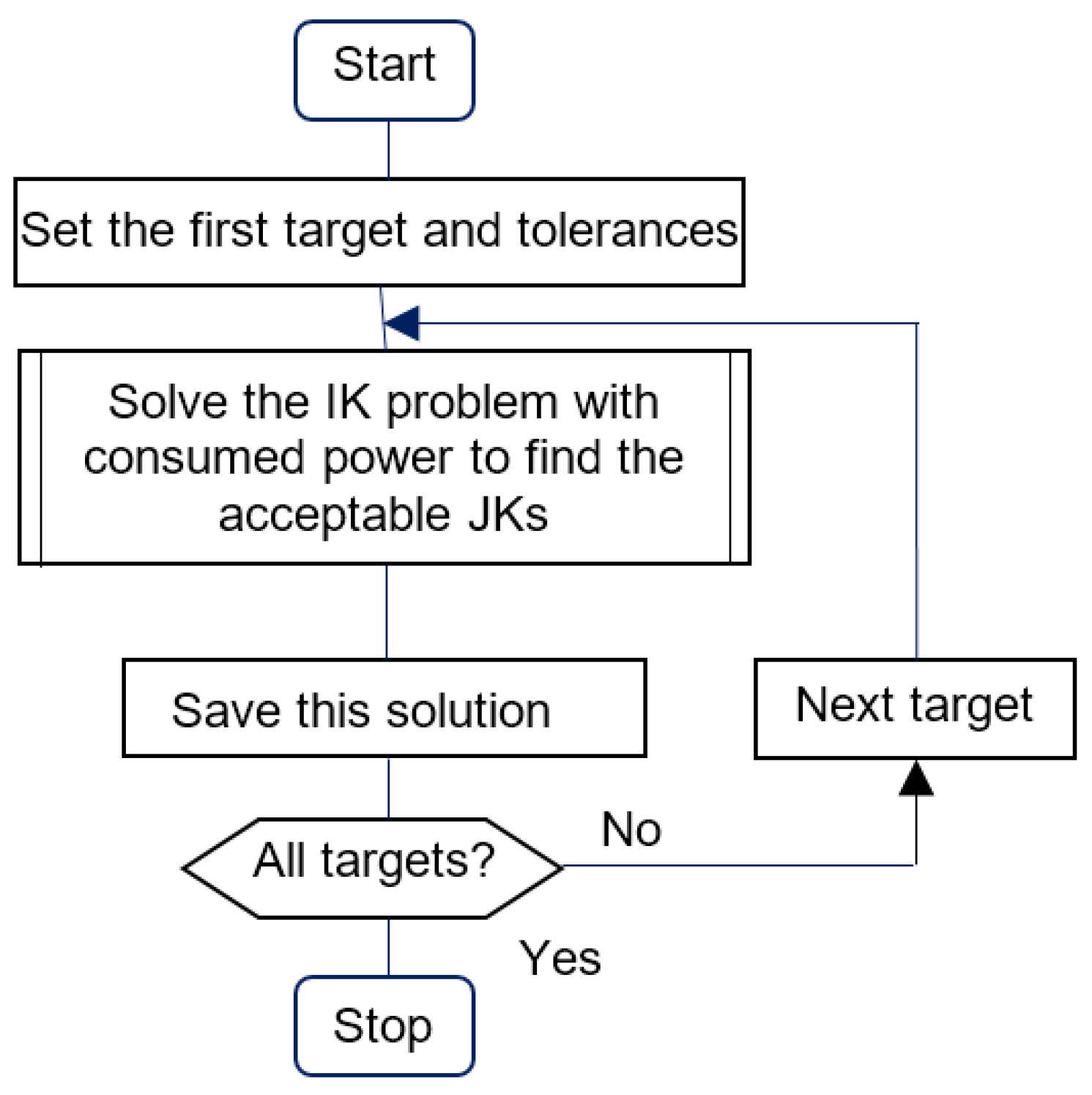
An appropriate algorithm is shown in
Figure 4. It has adjustable parameters, such as the X, Y, and Z Cartesian coordinates of the targets and the number of JKs in a target. Since the targets are usually not rigidly fixed into the desired locations but permit small accuracy tolerances, the acceptable errors between tool positions, generated based on the solution and the target position, are also specified.
Table 3 illustrates a case study in which a specific PnP process is described by 10 targets, corresponding to 10 Cartesian positions of X, Y, and Z, which the tool should pass with a 5% tolerance. In this example, each of the 10 targets can be reached using one of four JKs, with different A1, A2, and A3 joint coordinates and power demands, P, being found as solutions to the problem. The JKs with minimal consumed power are highlighted. In the last column, the amounts of saved power are calculated for each target. For example, to reach Target 1 (X = 37, Y = −32, Z = 163 mm), four JKs can be used, with different A1, A2, and A3 joint positions and different levels of power consumption being appropriate. The fourth configuration is the best since it requires 2.7% less power than the first one.
This PnP case study shows that by choosing an optimal JK, it is possible to reduce the static power consumption of the LDR slightly, mostly less than 3%. Such a reduction looks rather small compared to the 18% savings achieved in 6-DOF robots of serial architecture, as described in [
29].
4.3. Planning an Energy-Optimal Path for Joints
In accordance with (6), another way to save energy is by shortening the total joint route distance through all targets, considering all possible JKs at which the overall energy consumption becomes minimal as a result of time reductions in the PnP process.
The developed NN-based model opens up new possibilities for finding the shortest path that the joints A1, A2, and A3 might follow between the given picking and placement positions in the PnP tasks, which are similar to those shown in
Table 3.
Many mathematical methods, such as the Floyd–Warshall algorithm and different variations of Dijkstra’s algorithm, are used to find solutions to the shortest path problem [
33]. The peculiarity of the present task is its objective function (6), which represents the minimum of the total distance through all targets considering all possible JKs in the target.
The following solution is offered to this aim.
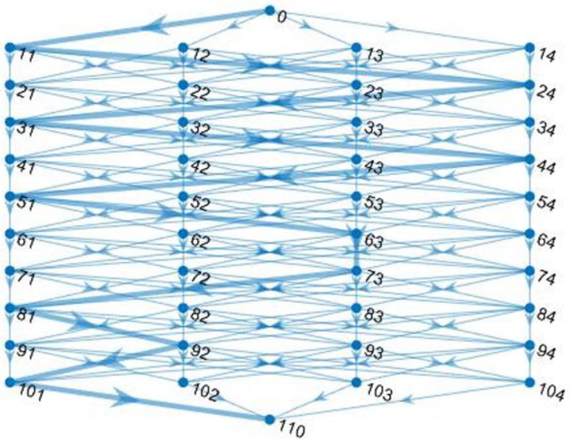
Let the desired PnP route passes via k targets, each of which can be achieved using one of p possible JKs. A {k to p2}-size array represents all possible distances between the candidate joints. Each distance is calculated as a maximal offset between conforming positions of joints A1, A2, and A3 in the neighbouring targets and labelled as “11”, “12”,…, “1p”, “21”,…, “kp”, where the first digit specifies the target number and the second one is the JK number in the target.
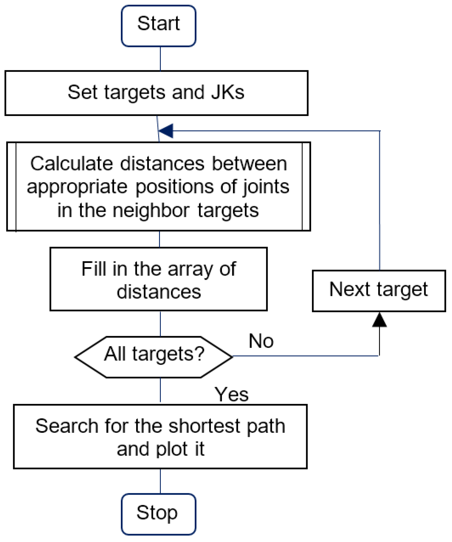
To search for and plot the shortest path, the “shortestpath”, “digraph”, “highlight”, and “printpath” MATLAB functions are applied. An appropriate algorithm is presented in
Figure 5.
Figure 6 demonstrates an example of the shortest path found for 10 targets with 4 possible JKs, each given in
Table 3.
In
Figure 6, the shortest path between targets 1 and 10 passes via the joint positions 11, 24, 31, 44, 51, 63, 73, 81, 92 and 101. The distances passed by joints are collected in
Table 4.
The total length of the found path is 1298 mm. Given an average joint velocity of 250 mm/s and an average consumed power of 250 W, the total energy needed to pass this route may be estimated to be 1298 J according to (6). In comparison with the longest path, up to 20% energy may be saved in this PnP task.
As follows from the diagram showing the shortest path, this route does not necessarily pass through the same JKs that are highlighted in
Table 3. This is due to the fact that another problem is formulated in this section, namely, searching for the shortest route between the JKs of all targets. The overall energy consumption drops here due to reductions in the total PnP process time.
4.4. Implementation Notes
For operating and programming Festo robots, the Festo Configuration Toolbox (FCT) is commonly used, which converts Cartesian coordinates X, Y, and Z into joint coordinates A1, A2, and A3, ignoring any energy indicators. The presented novel optimization routines seamlessly interface with FCT, which allows us to automatically compute energy-effective motion parameters. The designed IKP model helps to present the required PnP task in the form of a joint control program pre-processed from the Cartesian coordinates, thus implementing the proposed approach without FCT 2.2.0.97 software modification.
A more effective method could be to modify the toolbox by including the NN in the FCT software. In this case, the required PnP task might be prepared in the form of the Cartesian program, with its automatic processing by the system taking into account energy indexes. However, as it is correctly noticed in [
34,
35], most industrial robots are equipped with closed controllers, which heavily limits the feasibility of the offered method.
A test conducted on the LDR shown in
Figure 1 demonstrated a slight (2.5%) instability in terms of consumed energy in statics and a significant energy saving of 9.5% resulted from path optimization.
Figure 7 displays an experimental plot of phase power consumption obtained with the help of the Fluke 1745 power quality logger during the 67 s cycle of robot motion along the route shown in
Table 4. Here, the average power consumption of one phase is about 70 W, while the total power of the entire system is at least three times higher, at roughly 250 W. This result was compared with the result obtained by using a non-optimal path; in the latter case, the cycle lengthened up to 74 s with an appropriate energy demand growth.
The fact that the energy consumption of the separate drives that comprise LDRs is contingent upon the specific task at hand, namely, the targets of the motion trajectory, is worthy of attention. In particular, the points at the edge of the workspace, situated in the vicinity of the singularity, typically necessitate the operation of some drive at maximum power, while others may consume minimal power at any given instant. Moreover, the robot manipulability parameters are worthy of consideration in this context. The mass of the processed object, its form, and the manner in which it is gripped may significantly modify the torques of the drives, thereby influencing energy consumption. This means that, any time when the above parameters change, either the model has to be trained again or the designers must anticipate such situations in advance and save the relevant data in the model beforehand.
The same applies to any physics–mathematical model. However, the benefit of the NN models is that the designer does not need to search for the reasons for changes in robot physical data. For this actor, the LDR is a “black box” whose input and output data change, and the designer’s task is to measure new information in time and send it to the ready-made model.
Certainly, the authors did not check all scenarios considering laboratory restrictions. In the described case study, the power quality logger estimated the power consumption of all drives, and then the total power consumed was counted, considering additional system components loss. The goal of the experimentation was to verify the suggested method and to confirm its flexibility and saving rate, although in other conditions the numerical results will undoubtedly be different. In any case, they should be positive in terms of energy savings.
5. Conclusions
During production planning, it becomes crucial to minimize the energy costs of PnP operations, aiming to find the most economical technology. This paper presents a novel NN-based management approach for LDRs that are interfaced with robot programming tools which allow us to choose optimal sequence of operations in order to reduce total energy consumption. Here, the mathematical formulation of the problem is given and the design procedure of NN computer models of LDRs is reported. Based on these models, a search for the JKs with the lowest power demand is arranged. Then, a technique is established for planning the shortest route that the joints pass between the given initial picking and final placement positions in the total PnP process, following which the robot consumes the lowest amount of energy. Experimental tests performed on a Festo EXPT-45-E1 robot confirm the effectiveness of both the models and the appropriate simulation tools. An important advantage of this approach, as compared to the other ones not conceived of for energy saving, is that the optimal JK and tool path can be calculated just before the program is put into use.
The result of the study is applicable to both the novel and existing robotic systems, since the required modifications are limited to operation rescheduling and no investments are needed in new hardware.
Due to the relevance of the developed methodology, it might lead to similar solutions far beyond linear Delta robotics. However, given that energy consumption depends on the robot kinematics, statics, dynamics, workspace, and technical parameters, the usefulness of the proposed approach depends on the application, whether it is a process in which the holding power accounts the largest portion of the total power consumed by the robot, or it is a process in which rapid operation is required, as well as whether it is a multi-DOF serial robot or a 3-DOF parallel robot.

