Article

Linear Ensembles for WTI Oil Price Forecasting

by
João Lucas Ferreira dos Santos
1,†,
Allefe Jardel Chagas Vaz
2,†,
Yslene Rocha Kachba
3,†,
Sergio Luiz Stevan, Jr.
4,†,
Thiago Antonini Alves
2,† and
Hugo Valadares Siqueira
3,4,*,†
1
Graduate Program in Industrial Engineering (PPGEP), Federal University of Technology—Paraná, Ponta Grossa 84017-220, Brazil
2
Graduate Program in Mechanical Engineering, Federal University of Technology—Paraná, Ponta Grossa 84017-220, Brazil
3
Department of Industrial Engineering, Federal University of Technology—Paraná, Ponta Grossa 84017-220, Brazil
4
Graduate Program in Electrical Engineering, Federal University of Technology—Paraná, Ponta Grossa 84017-220, Brazil
*
Author to whom correspondence should be addressed.
These authors contributed equally to this work.
Energies 2024, 17(16), 4058; https://doi.org/10.3390/en17164058
Submission received: 25 June 2024 / Revised: 29 July 2024 / Accepted: 9 August 2024 / Published: 15 August 2024
(This article belongs to the Section C: Energy Economics and Policy)

Abstract

:
This paper investigated the use of linear models to forecast crude oil futures prices (WTI) on a monthly basis, emphasizing their importance for financial markets and the global economy. The main objective was to develop predictive models using time series analysis techniques, such as autoregressive (AR), autoregressive moving average (ARMA), autoregressive integrated moving average (ARIMA), as well as ARMA variants adjusted by genetic algorithms (ARMA-GA) and particle swarm optimization (ARMA-PSO). Exponential smoothing techniques, including SES, Holt, and Holt-Winters, in additive and multiplicative forms, were also covered. The models were integrated using ensemble techniques, by the mean, median, Moore-Penrose pseudo-inverse, and weighted averages with GA and PSO. The methodology adopted included pre-processing that applied techniques to ensure the stationarity of the data, which is essential for reliable modeling. The results indicated that for one-step-ahead forecasts, the weighted average ensemble with PSO outperformed traditional models in terms of error metrics. For multi-step forecasts (3, 6, 9 and 12), the ensemble with the Moore-Penrose pseudo-inverse showed better results. This study has shown the effectiveness of combining predictive models to forecast future values in WTI oil prices, offering a useful tool for analysis and applications. However, it is possible to expand the idea of applying linear models to non-linear models.

1. Introduction

The global energy consumption scenario is dominated by non-renewable sources such as coal, oil and natural gas. In 2022, according to the Energy Information Administration (EIA) [1], the consumption was: oil (29.5%), coal (26.8%), natural gas (23.7%), biomass (9.8%), nuclear energy (5.0%), hydroelectric energy (2.7%) and other sources (2.5%). In the coming years, oil and natural gas are expected to remain prominent, driven by the development of nations such as China, the largest importer and second largest consumer of oil [2].
Oil, a raw material with high industrial value, has its price influenced by global economic and geopolitical aspects [3,4,5,6,7,8,9]. This price is determined by a complex, non-linear system with many uncertainties [10].
Since 2008, the fall in oil prices has been influenced by the global economic slowdown and geopolitical instability, as well as the crisis between China and the US. The COVID-19 pandemic and the war between Russia and Ukraine have added new uncertainties, affecting price formation [6,11,12]. These events have caused fluctuations in prices, challenging market and political decisions, but also offering opportunities to explore forecasting methods.
Forecasting models include linear and non-linear approaches and combination strategies such as hybrids and ensemble. Linear models, such as exponential smoothing, are used to capture patterns in time series by adjusting for trends and seasonality. For example, Simple Exponential Smoothing (SES) is suitable for series with no trend or seasonality, while the Holt-Winters model deals with series that have these characteristics. Box & Jenkins models, such as AR, ARMA and ARIMA, are essential for analyzing time dependencies, where AR captures the linear relationship between an observation and several past lags, MA models the forecast error as a linear combination of past errors and ARIMA handles non-stationary series by incorporating differentiation [13].
Variants of the ARMA model optimized by Genetic Algorithm (GA) and Particle Swarm Optimization (PSO) improve forecast accuracy by automatically adjusting parameters, allowing for more effective modeling of complex dynamics [14]. These optimization techniques provide an enhanced ability to capture subtle patterns and deal with the inherent complexity of time series.
In addition to hybrid models, combination strategies such as ensemble combine outputs from individual predictors [15]. These strategies include averages, medians, weighted averages and other combinations [16,17]. ensemble techniques optimize the accuracy of forecasts by combining results from multiple models, reducing the variance of errors and increasing the consistency of estimates in volatile markets.
The literature has evolved regarding forecasting models for monthly crude oil (WTI) futures prices [18,19,20]. Although new techniques are emerging, linear models are still widely used, from simple comparisons to hybrid models [21].ensemble models have the potential to improve forecast accuracy, but are still little explored [15,16,17].
The aim of this article is to explore linear models, specifically smoothing and Box & Jenkins models, and apply incremental adjustments to the ARMA model using GA and PSO. Combination strategies ensemble considered include mean, median, pseudo-inverse of Moore-Penrose and dynamic adjustments of weights with GA and PSO, significantly improving the performance of the results.

2. Linear Models

2.1. Smoothing Models

This section presents the first set of models used, known as smoothing models. In these models, the main objective is to estimate the smoothing parameters. The models will be divided as follows: Simple Exponential Smoothing SES, Holt Exponential Smoothing (HES), Additive Holt-Winters (A-HW) and Multiplicative Holt-Winters (M-HW).

2.1.1. Simple Exponential Smoothing (SES)

Simple Exponential Smoothing SES is a data smoothing model that applies non-corresponding weights to the fundamental values of the time series [22,23]. The forecast for one period ahead is given by Equation (1):
F ^ t + 1 = α x t + ( 1 α ) · F t
where F t + 1 is the forecast, x t is the actual data in period t, F t is the forecast in period t and α is the smoothing parameter ( 0 < α < 1 ).
Values of α close to zero indicate slower forecasts and less reaction to changes, while values close to one result in faster responses to recent changes in the time series.
After defining the SES model equation, the next section will introduce the Holt model.

2.1.2. Holt Exponential Smoothing (HES)

The Holt Exponential Smoothing HES models are widely used in time series with a linear trend [24]. Unlike the SES model, which smooths only the level, the Holt model also models the trend. Represented by Equations (2)–(4).
L t = α Z t + ( 1 α ) · ( L t 1 + T t 1 )
T t = β ( L t L t 1 ) + ( 1 β ) T t 1
Y ^ = L t + T t
where L t is the new smoothed value, α is the smoothing coefficient ( 0 < α < 1 ), Z t is the current value in period t, β is the trend smoothing coefficient ( 0 < β < 1 ), T t is the predicted trend, and Y ^ is the predicted value.
Low values of β indicate a slow adjustment to the trend, while high values indicate a rapid response to changes in the trend.
The next section will introduce the Holt-Winters model, which models seasonality in an additive or multiplicative way.

2.1.3. Holt-Winters Model

The Holt-Winters model, or triple smoothing model, is used for data with trend, level and seasonality [25]. This model has two variations: Additive Method and Multiplicative Method.
Additive Holt-Winters Method (A-HW): Represented by Equation (5):
Z t = L t + T t + S t + ε t
where L t is the level, T t the trend, S t the seasonality at time t and ε the white noise. The estimates of the model components are given by Equations (6)–(8):
T ^ t = β ( L t L t 1 ) + ( 1 β ) T t 1
L ^ t = α ( Z t S t 1 ) + ( 1 α ) ( L t 1 + T t 1 )
S ^ t = γ ( Z t L t ) + ( 1 γ ) S t 1
where α , β and γ are the smoothing parameters for level, trend and seasonality ( 0 < γ < 1 ).
Multiplicative Holt-Winters Method (M-HW): Represented by Equation (9):
Z t = ( L t + T t ) S t + ε t
The estimates of the model components are given by Equations (10)–(12):
L ^ t = α Z t S t 1 + ( 1 α ) ( L t 1 + T t 1 )
T ^ t = β ( L t L t 1 ) + ( 1 β ) T t 1
S ^ t = γ Z t L t + ( 1 γ ) S t 1
Additive models are indicated for seasonal variations of constant amplitude [26], while multiplicative models are suggested for increasing or decreasing seasonal variations [27]. Both models were tested in this study. The next section will present the adjustments of the smoothing models.
After presenting the smoothing models, the next section will introduce the Box & Jenkins models and their variations.

2.2. Box & Jenkins Models

The Box & Jenkins models, such as ARIMA( p , d , q ), are notable for their accuracy in forecasting time series [25,28,29]. In addition to ARIMA, there are AR(p) and ARMA( p , q ) models, and the challenge is to determine the values of (p), (d) and (q) and their respective coefficients [30].
Next, the AR(p), ARMA( p , q ) and ARIMA( p , d , q ) models are discussed.

2.2.1. Autoregressive Model—AR(p)

The AR(p) model uses p time lags as inputs to forecast future observations, represented by the linear combination Z ^ t 1 + + Z ^ t p  of the past terms of the series, multiplied by the coefficients ϕ p and adding a Gaussian white noise a t [13,31]. Based on a deterministic approach, AR(p) uses the Yule-Walker Equations to estimate its coefficients, minimizing the error between the observed data and the predictions [28]. Equation (13) represents the model.
Z ^ t = ϕ 1 Z t 1 + ϕ 2 Z t 2 + + ϕ p Z t p + a t
where Z t is the predicted value at time t, ϕ p is the weighting coefficient for the delay of p 1 , 2 , , P .
Direct application of this model requires stationary data.

2.2.2. Autoregressive Moving Average Model—ARMA(p,q)

The ARMA( p , q ) model combines autoregression (AR) and moving average (MA) components [13,32]. Equation (14) describes the model:
Z ^ t = ϕ 1 Z t p + ϕ 2 Z t p 1 + + ϕ p Z t p p + 1 θ 1 a t 1 θ 2 a t 2 θ q a t q + a t

2.2.3. Autoregressive Integrated Moving Average Model—ARIMA(p,d,q)

The ARIMA( p , d , q ) model extends ARMA with an order of differentiation d to remove trends and make the series stationary [33]. Equation (15) describes the model:
Z ^ t = ϕ 1 Z t 1 + + ϕ p Z t p θ 1 ε t 1 θ q ε t q ε t
The direct application of the ARIMA model makes it possible to model random shocks using the forecast error from the previous step ε t 1 , where ε t = a t .
Maximum likelihood estimation can be used to determine the θ coefficients of the ARMA( p , q ) and ARIMA( p , d , q ) [34] models.

2.3. Bioinspired Optimization Tools

In this section, we present the algorithms used to optimize the ARMA( p , q ) models, using two different strategies: Genetic Algorithms GA and Particle Swarm Optimization PSO. The details of how these algorithms were applied to the problem in question will be provided in Section 3 along with the application of the Ensemble model.

2.3.1. Genetic Algorithms (GA)

Optimization using Genetic Algorithms GA is widely used among algorithms inspired by biological processes. Based on the principles of the theory of evolution of Darwin [35,36,37], GAs model biological behavior to solve optimization problems. Introduced by [38] and refined by [39,40], GAs are recognized for identifying optimal or suboptimal solutions, and are robust to various problems, as they seek a global optimal solution [41].
In the context of GAs, the problem is modeled by representing individuals associated with the parameters and coefficients of the models to be optimized, evaluated by the degree of adaptability, known as fitness [14]. This establishes an analogy between an individual’s ability to thrive in an environment and the effectiveness of parameters in producing an optimal solution.

2.3.2. Particle Swarm Optimization (PSO)

A major advantage of metaheuristics is that they are derivative-independent, unlike classical optimization techniques such as gradient descent or Newton methods, which require derivatives of the predictor [42]. This makes them especially useful in problems where derivatives are unavailable or difficult to calculate.
Inspired by the social behavior of birds and fish, Particle Swarm Optimization PSO, proposed by [35], uses individual and collective experience to solve problems. PSO limits the distribution of swarm members in the search space by the current position ( x p ) and velocity ( v p ) [43]. The search for the best solution is guided by improving the local position ( p b e s t ) and the best global position ( g b e s t ).
Reference The authors [44] proposed adding the inertia coefficient ( ω ), according to Equation (16), restricting the area surveyed. Values of ω vary from 0.9 for broad searches to 0.4 for narrow searches, affecting convergence. Cognitive components c 1 and c 2 influence the solution using past experiences, initially defined as 2 [44].
v p ( i + 1 ) = ω v p ( i ) + c 1 · rand 1 ( i ) [ p b e s t p x p ( i ) ] + c 2 · rand 2 ( i ) [ g b e s t p x p ( i ) ]
The performance of the PSO is influenced by c 1 and c 2 , controlling the speed and direction of the search. When the swarm starts, the particles are randomly distributed in the search space. Each particle is evaluated by the fitness function; the best position found is stored in ( p b e s t ) and ( g b e s t ). The speed of each particle is updated in each iteration based on ( p b e s t ) and ( g b e s t ), until the stopping criterion is reached.
After defining the linear models and optimization tools, the next section presents the Ensemble strategies used.

2.4. Tools for Combining Predictors Ensemble

One of the main advantages of ensembles lies in the ability to synergistically combine different individual models, which can result in remarkable improvements in the generalization process and in the accuracy of predictive models, as mentioned by [45,46,47]. Therefore, it can be said that a Ensemble has the ability to reduce error variance.
However, it is important to note that the effectiveness of ensembles is directly linked to the assertiveness of the individual models, which is influenced by the combination method adopted, as pointed out by [48]. There is no definition or consensus on which ensemble strategy should be used [49].
An ensemble can consist of several stages, such as the generation of individual models, the selection of models and, finally, their combination or aggregation [50,51].
The model generation stage is crucial for creating diversity within the Ensemble [51]. It can be classified as heterogeneous, using models with different architectures, or homogeneous, using models with the same architecture [50,52]. The combination of both approaches is common to diversify the Ensembles [53,54], although heterogeneous models can face challenges in maintaining diversity [53]. Homogeneous models, on the other hand, offer greater control over diversity [53].
The selection and combination of models are fundamental steps in the process of forming an ensemble, with the aim of balancing diversity and forecast accuracy. After generating the models, the next stage is selection, which is essential for building an efficient Ensemble.
A fundamental part of the composition of an ensemble is the selection of predictors, which can involve choosing all the available predictors or a specific subgroup, following established criteria. Selection can be static, using one model or subgroup for the entire test set [55,56], or dynamic, choosing models based on the region of competence during the test phase [50,57]. Although selection is not mandatory at this stage, it can influence the results. Considering all predictors for the final stage may be prudent to avoid selecting models that may underperform in the test set [57]. The next step in forming an Ensemble is the final combination of predictors.
This step integrates the results of the forecasts of the individual predictors, forming the Ensemble forecast ( Z ^ t + 1 ). In time series problems, it is common to aggregate the forecasts of k predictors to obtain more accurate results, usually using the mean or median of the forecasts [58,59].
Both the mean and the median are non-trainable ensemble models, reducing computational costs as it is not necessary to retrain the models repeatedly. The mean is represented by Equation (17), where y i are the predictions of the predictor i and m is the total number of predictors.
Z ^ t + 1 = 1 m i = 1 m y i
The median, represented by Equation (18), is useful in the presence of outliers, offering a robust estimate of the central tendency of the forecasts.
Z ^ t + 1 = Median { y 1 , y 2 , , y m }
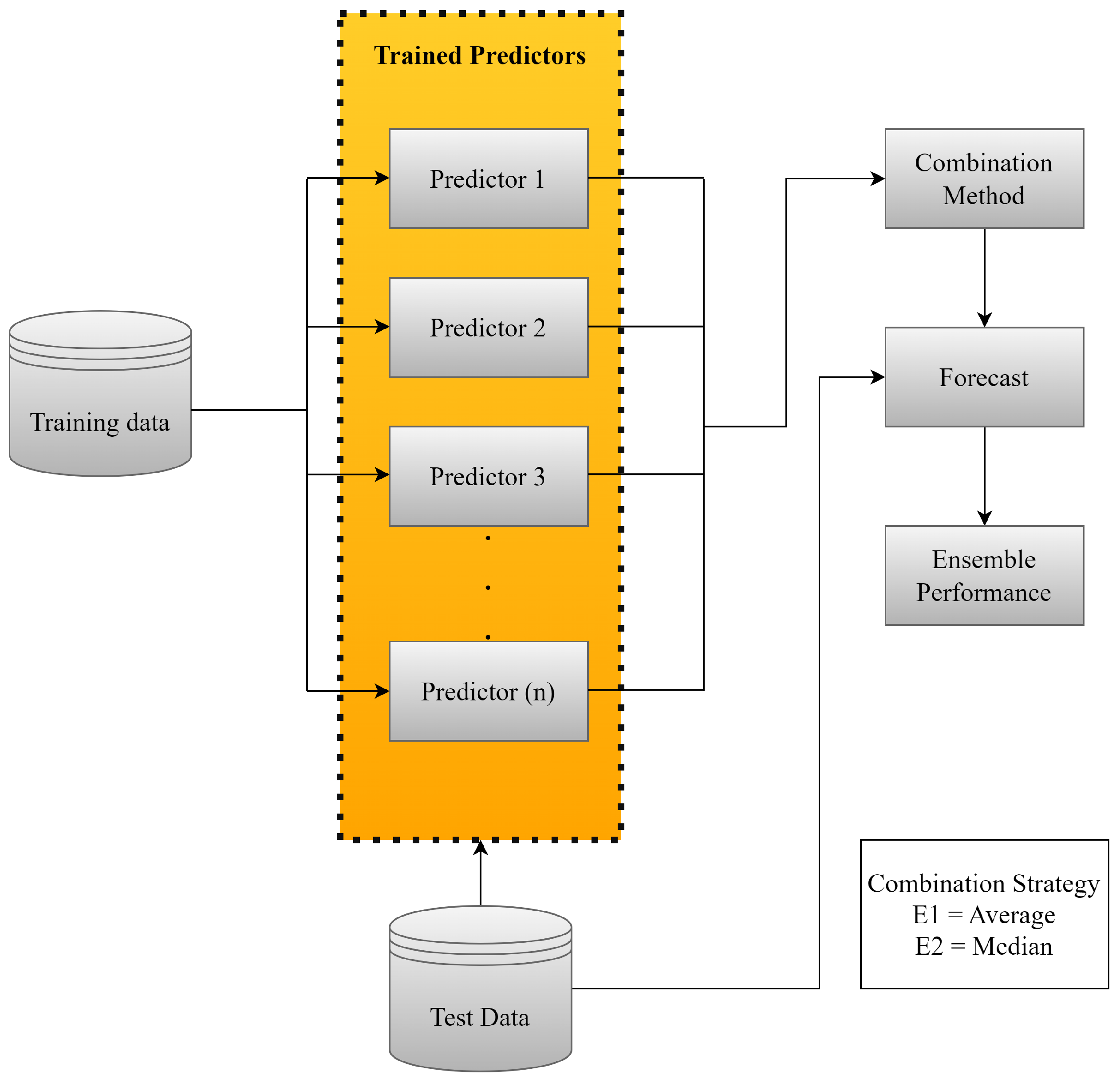
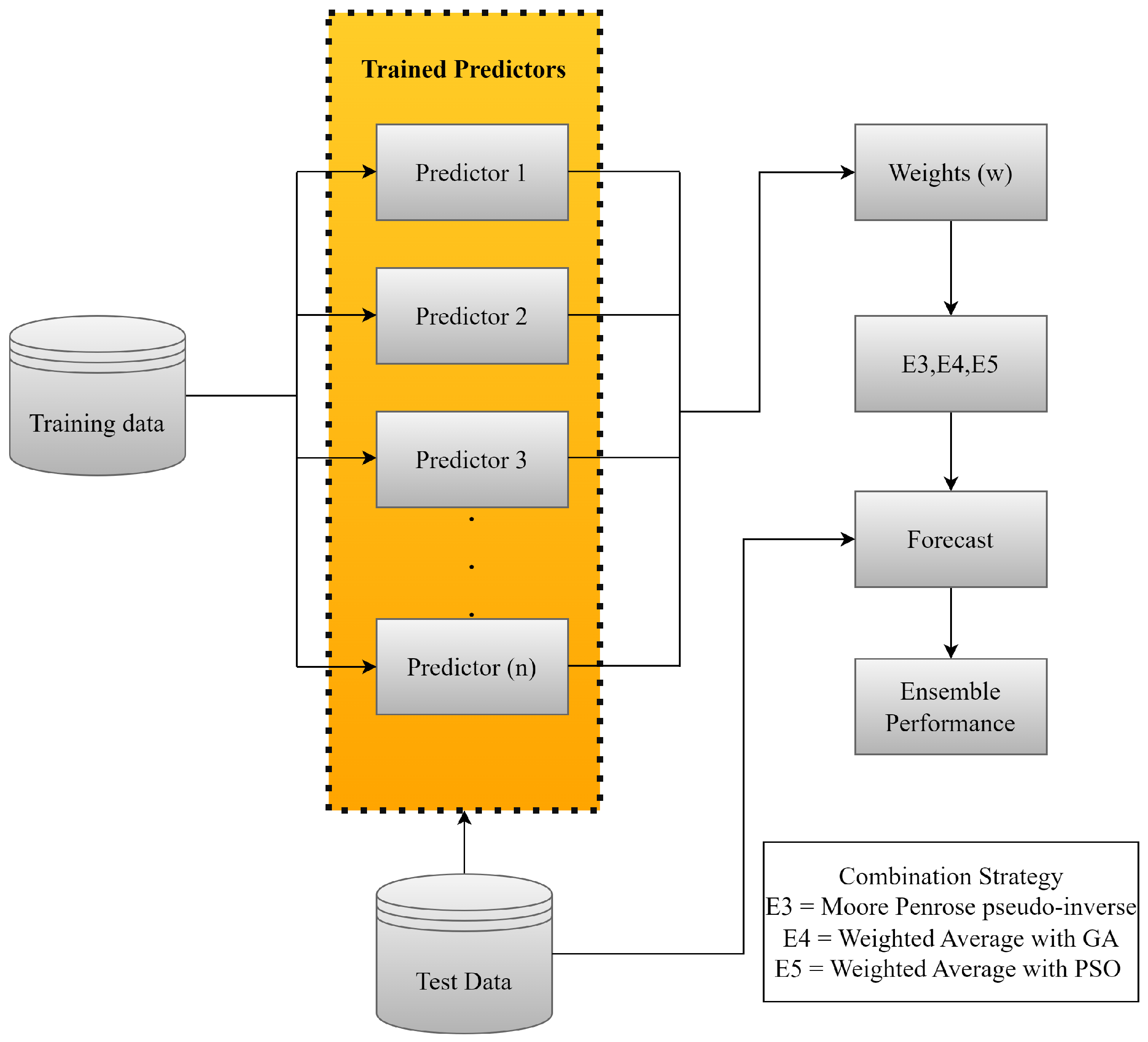
Figure 1 illustrates the process of combining previously trained models using a non-trainable approach.
In addition to the non-trainable ensembles, we also investigated the trainable ones, which differ in the assignment of weights to each predictor [60,61]. This stands out as the main contribution of this research.
Weights can be determined in various ways, such as minimum, maximum or product of the predictors’ outputs. A viable strategy is the weighted average, assigning greater weights to the models with the best performance [62,63,64].
The pseudo-inverse of Moore-Penrose can be used to calculate the weights, effectively adapting to the characteristics of the predictors [65]. Equation (19) provides the solution to this problem:
W = ( Y T Y ) 1 Y T y
Figure 2 shows the procedure for combining previously trained models, incorporating an additional re-training step.
This additional step adjusts the weights of the ensemble models according to the evolution of the data or problem conditions, resulting in a trainable approach.
In this paper, we propose an ensemble of predictive models, where the final output is calculated as the weighted average of the models’ individual predictions, represented by Equation (20).
y ^ = i = 1 M w i · y ^ i ,
The weights w i are optimized using Genetic Algorithm GA and Particle Swarm Optimization PSO, in order to minimize the prediction error of the ensemble [66].
After defining the linear models, optimization and combination tools, the next section will present the evaluation of these steps.

3. Methodology

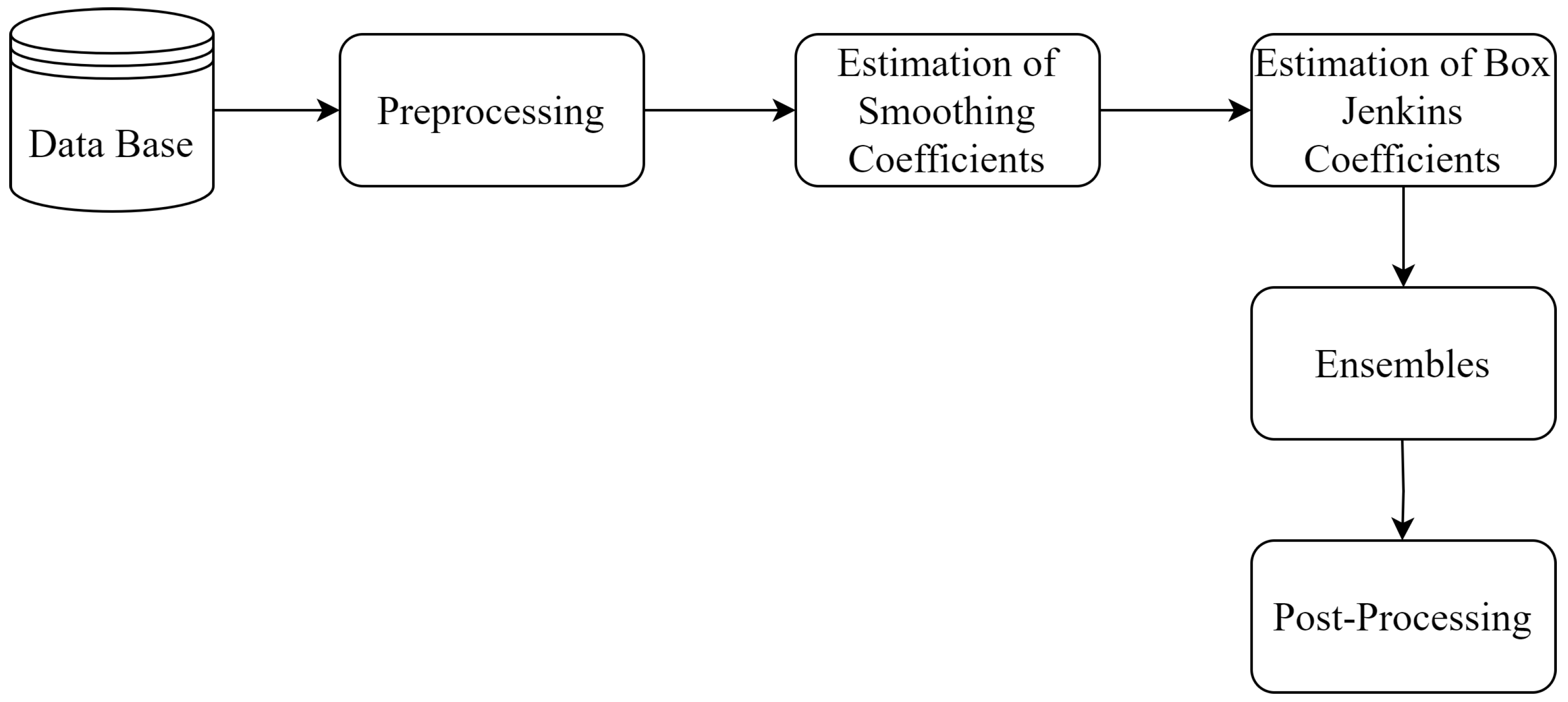
In this section, the stages for the development of this research will be presented. Figure 3 illustrates the organization of the stages.
All the statistical tests and computational results were developed using the Python 3.11.5 version programming language.

3.1. Database

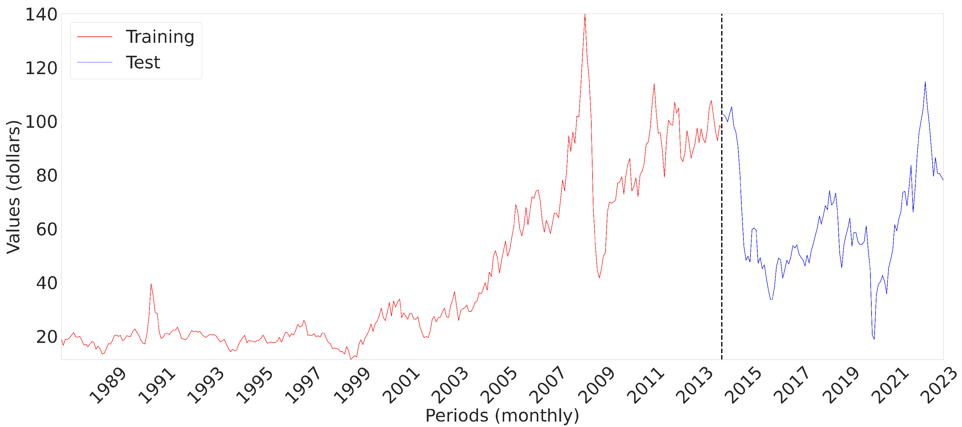
The data analyzed, from the EIA [1], covers the monthly closing prices of WTI crude oil from January 1987 to February 2023, totaling 434 observations and showing total integrity with no missing or null records. The distribution of this data is illustrated in Figure 4.
To develop the models, 75% of the data was used for training, while the remaining 25% was used for testing, as shown in Figure 4.

3.2. Pre-Processing

After collecting the data, it was analyzed to identify behaviors such as trend, cyclicality, seasonality and a random term. One of the ways to detect these behaviors is to use certain tests, such as the Cox-Stuart test and the Friedman test [67,68].
The tests show that the series has a trend and seasonality. In this case, it is necessary to pre-process the data to ensure stationarity. The so-called stationary series have a constant mean, constant variance and autocovariance that does not depend on time, reflecting a more stable behavior of the data, which for modeling, especially the Box & Jenkins models, is a sine qua non condition [25,28,69].
For this study, we used the logarithmic transformation and the moving average with a 12-month window, along with differentiation, as shown in Equations (21)–( 23).
L ( t ) = log ( Z ( t ) )
in this case L ( t ) will be the value of the logarithm, Z ( t ) represents the time series at time t.
M ( t ) = 1 N k = t n + 1 t L ( i )
and M ( t ) represents the value of the moving average at time t. The moving average is calculated as the average of the L ( i ) values with a window of N-periods. Now ( i ) represents the iteration over all the points in the N-period window.
If we then apply differentiation using Equation (23), you get:
Δ = ( L ( t ) M ( t ) ) ( L ( t 1 ) M ( t 1 ) )
Combining all the parts, the complete transformation of the time series is represented by Δ .
The next step is to determine the parameters of the smoothing models. In this case, determine the parameters for level, trend and seasonality.

3.3. Estimating the Smoothing Coefficients

Exponential smoothing models require the determination of the α , β and γ coefficients. The literature indicates that there is no consensus on an ideal method for this determination [70]. Using the numerical evaluation of the cost function, the L-BFGS-B (The standard algorithm in the statsmodels library minimizes the mean square error (MSE) using the Quasi-Newton method, without the need to provide the Hessian matrix or the structure of the objective function) method was used to minimize the MSE and define the parameters in the training set.
Although Exponential Smoothing models do not require the series to be stationary, it was decided to use stationary data in this study. The adjusted parameters α , β and γ are shown in Table 1 and Appendix A.
After determining the coefficients of the smoothing models, we proceeded to apply the Box & Jenkins models.

3.4. Estimating the Coefficients and Orders of the Box & Jenkins

For the Box & Jenkins models, the orders and coefficients were determined in two ways: the classical approach and the optimization of the coefficients of the ARMA( p , q ) model using GA and PSO.
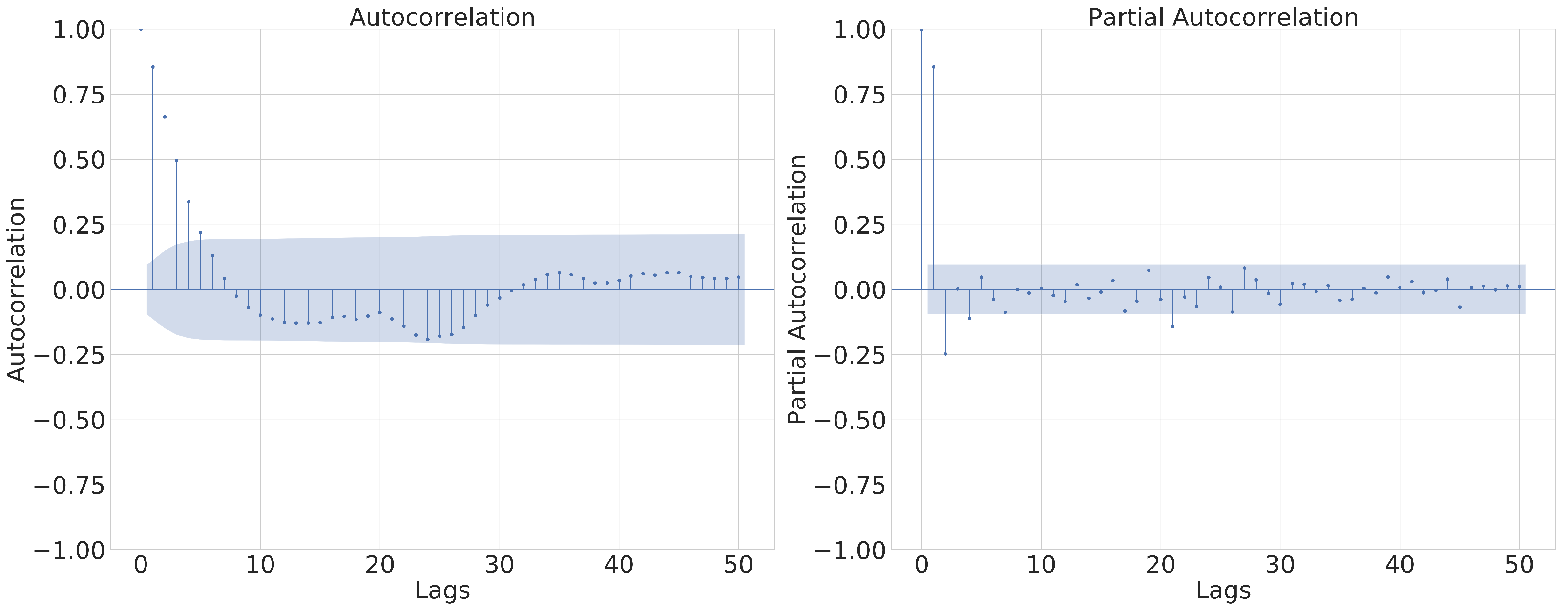
The candidate orders were evaluated using the Autocorrelation Function (ACF) and Partial Autocorrelation Function (PACF) graphs. The θ i coefficients were estimated by solving the Yule-Walker Equations for AR(p) [71]. For the ARMA( p , q ) and ARIMA( p , d , q ) models, the maximum likelihood estimator [34] was used. The d part of the ARIMA model was determined as 1 by applying a differentiation to the data.
Significant lags were defined by analyzing Figure 5, which makes it easier to understand the autocorrelation patterns in the adjusted time series.
The ACF and PACF help identify significant lag components for the AR and MA models, respectively [72]. Determining these parameters can be challenging due to the complexity and volume of the data. For the AR(p) model, although Figure 5 suggests testing up to lag 2, lags from 1 to 6 were observed. For the ARMA( p , q ) model, the MA(q) part was tested up to order 6, as indicated by the ACF.
For the ARIMA( p , d , q ) model, the same orders were tested, with d set to 1. The coefficients of the Box & Jenkins models are shown in Table 2. After analyzing the orders, it was decided to refine the choice of parameters, especially for the ARMA( p , q ) model, using GA and PSO optimization for greater precision [73,74].
Siqueira2 Table 3 and Table 4. In GA, the parameters ϕ and θ were optimized with p = 1 and q = 3 , using one-point crossover, dynamic mutation and roulette wheel selection. The specific parameters are detailed in
In PSO Table 4, particles represent candidate solutions ( ϕ 1 , θ 1 , θ 2 , θ 3 ) R . The particles adjust their trajectories based on the best individual ( p b e s t ) and global ( g b e s t ) experiences. The inertia (w), cognitive ( c 1 ) and social ( c 2 ) coefficients modulate the search dynamics. 30 simulations were carried out to identify the optimal configuration.
The optimized values of ( ϕ 1 , θ 1 , θ 2 , θ 3 ) R are shown in Table 5. With the application of GA and PSO, all the linear models are ready to be combined. The ensembles can be developed using the techniques presented in Section 2.4.

3.5. Ensemble

To build ensemble 1, the average of the models’ forecasts was used, as described in Equation (17), for the forecast horizons of 1, 3, 6, 9 and 12 steps ahead. The forecasts were collected and the arithmetic mean was calculated, with all model outputs contributing equally to the final forecast, without the need for readjustment or retraining. Individual errors were calculated for each horizon.
Ensemble 2 was developed based on the median of the models’ forecasts, following the same steps as ensemble 1 and using Equation (18). Each model was evaluated individually.
Ensemble 3, unlike ensembles 1 and 2, is trainable. Initially, the model predictions were organized in a Y matrix and the actual values in a y vector. The weights that minimize the quadratic difference between predictions and actual values were calculated by applying the pseudo-inverse of Moore-Penrose to solve the least squares problem Equation (19).
For ensemble 4, the weighted average of the models’ predictions was used, with weights initially optimized using GA. A chromosome was formed representing the weights W, with the restriction that the weights add up to 1 and are non-negative. GA was applied with one-point crossover, dynamic mutation and tournament selection, as detailed in Table 6.
After simulations and tests with GA, the parameters for PSO were defined Table 7. Each particle in the PSO represents a candidate solution and adjusts its trajectory based on the best individual ( p b e s t ) and global ( g b e s t ) experiences, following Equation (16).

3.6. Post-Processing

After the initial transformations to the time series data, it was necessary to reverse the modifications to recover the “removed” values and return the forecasts to the original scale. This makes it easier to understand and visualize the results accurately, ensuring that the accuracy metrics are on the same scale as the original data.
The following evaluation metrics were used: MSE, MAE, MAPE and AE.
The Mean Square Error MSE calculates the average of the squared errors with Equation (24).
M S E = 1 n t = 1 n ( y y ^ ) 2
The Mean Absolute Percentage Error MAPE avoids different scale penalties, represented with Equation (25).
M A P E = t = 1 n | y y ^ y ^ |
And the Mean Absolute Error MAE calculates the average of the absolute errors with Equation (26).
M A E = 1 n t = 1 n | y y ^ |
On the other hand, the Absolute Error AE is the difference between the observed value and the predicted value and can be calculated with Equation (27).
A E = | y y ^ |
Section 4 will present the final results with the models adjusted and reversed as described in Section 3.6.

4. Results

This section presents the results of the models evaluated for each forecast horizon, based on the MSE, MAE and MAPE errors, followed by a ranking of the models (Table 8). For each horizon, the best result is illustrated next to the actual data, as well as the Absolute Error AE curves over time for the 14 models evaluated.The graphs are organized as follows:
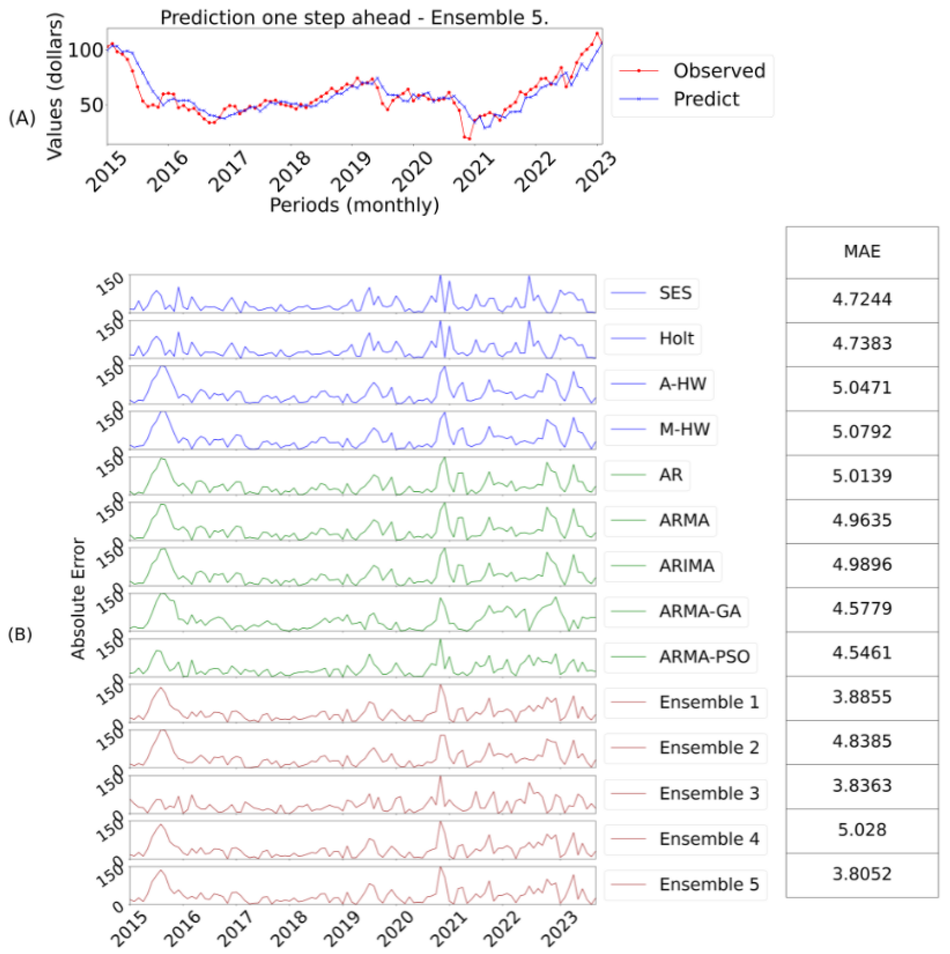
  • Figure 6: A corresponds to the prediction of the best model and B o the evaluation of the AE for one-step ahead;
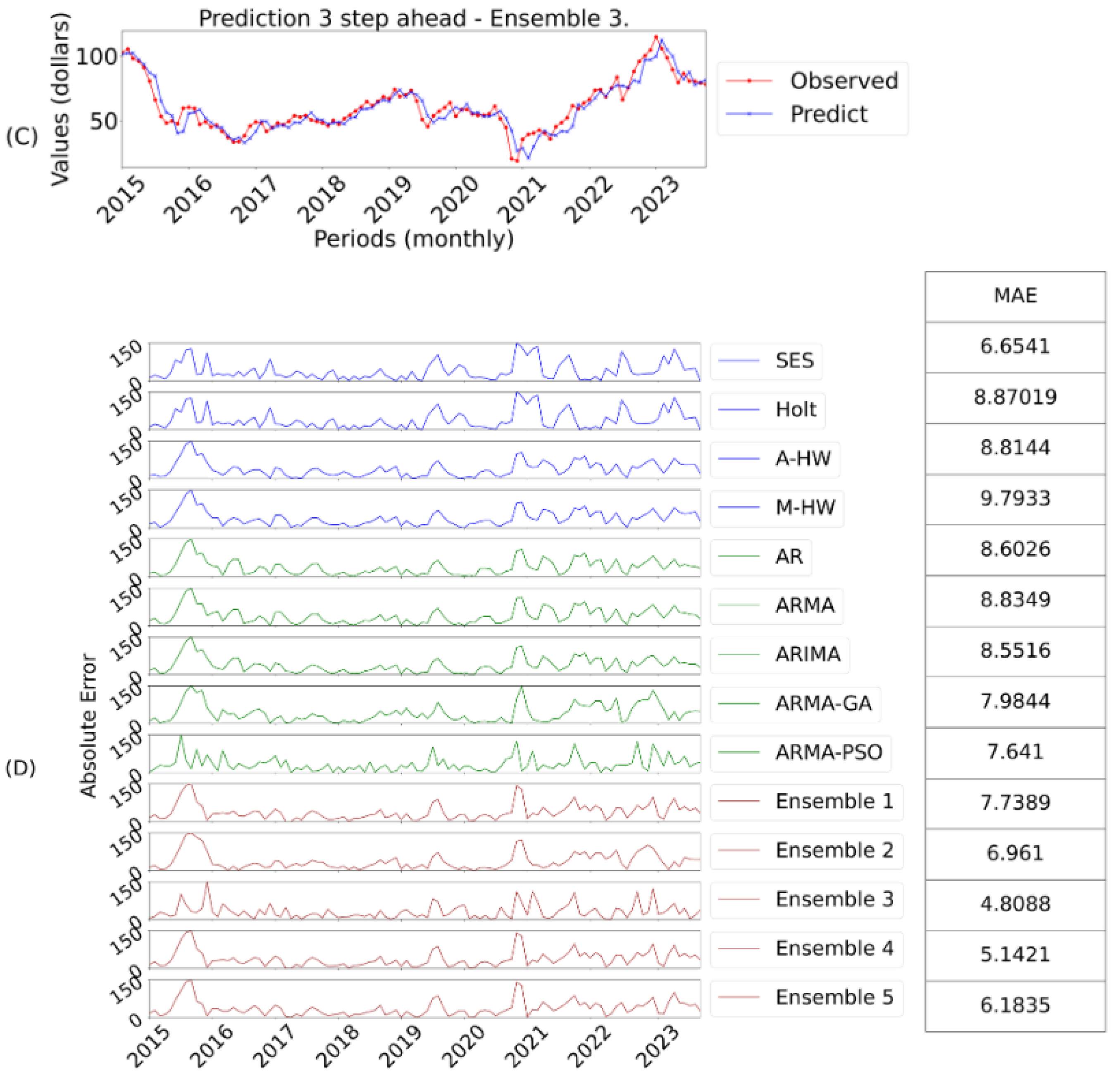
  • Figure 7: C represents the prediction of the best model and D the AE evaluation for three-steps ahead;
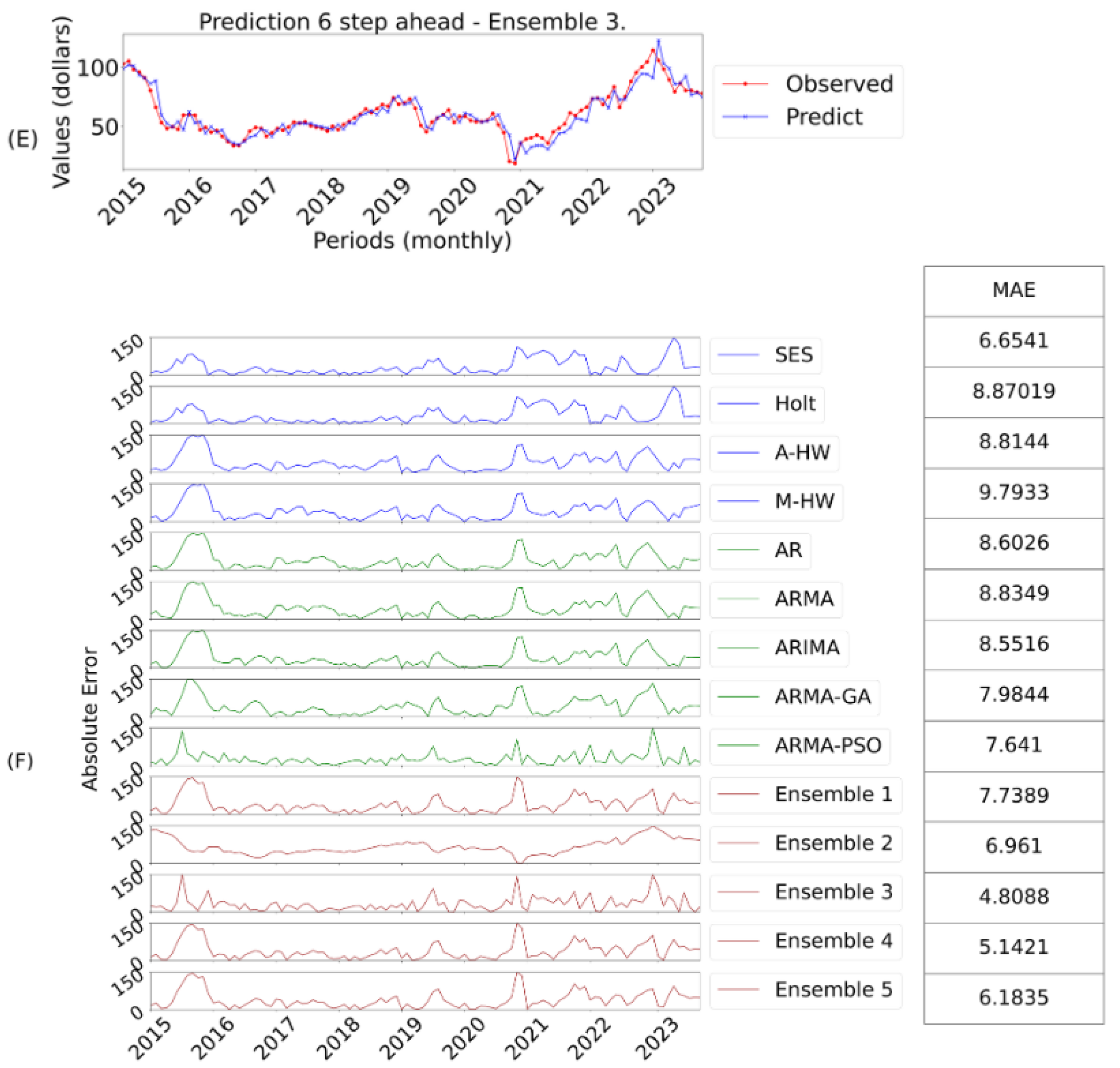
  • Figure 8: E shows the prediction of the best model and F the AE evaluation corresponding to six-steps ahead;
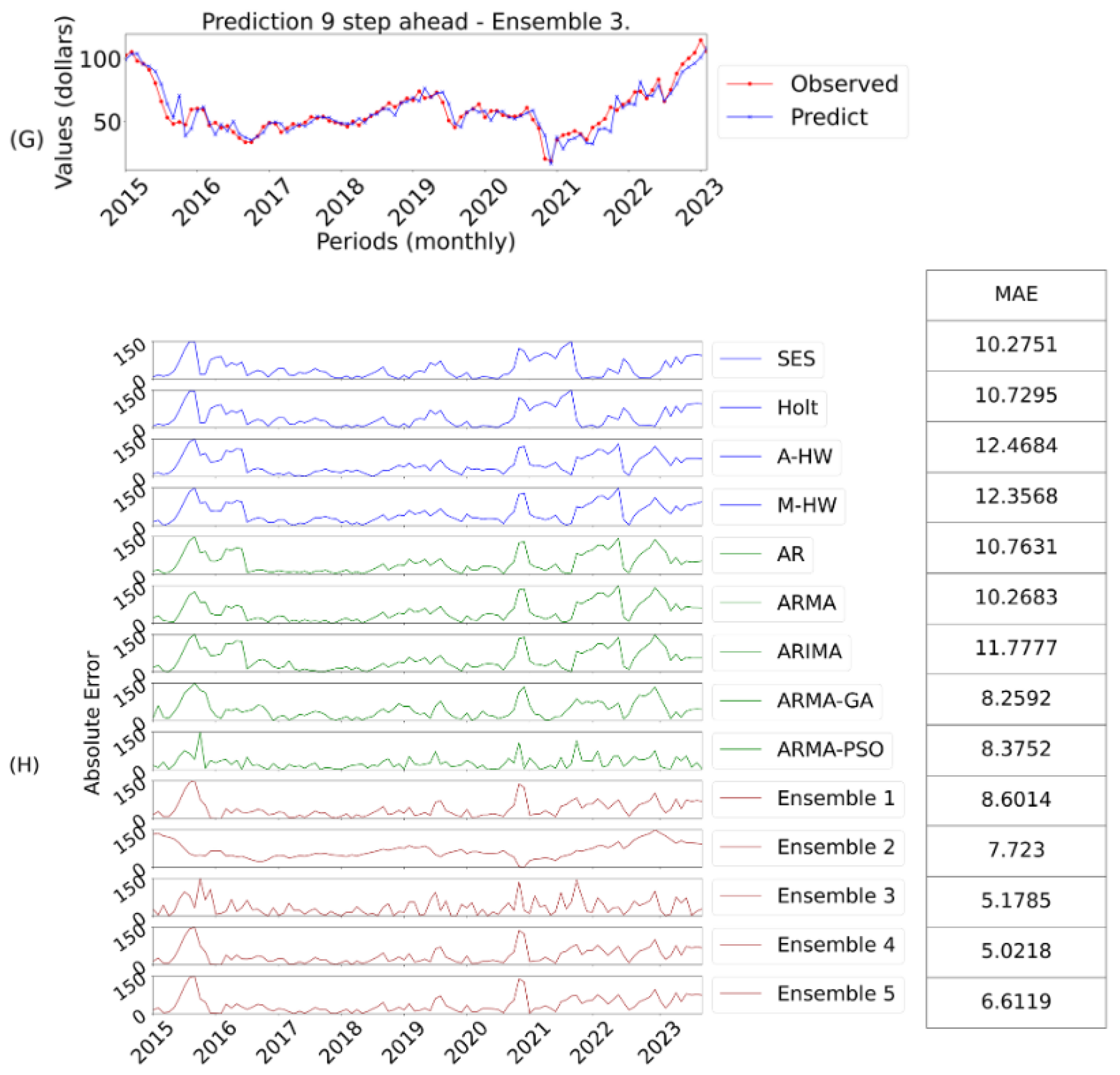
  • Figure 9: G shows the best model prediction and H the AE evaluation for nine-steps ahead;
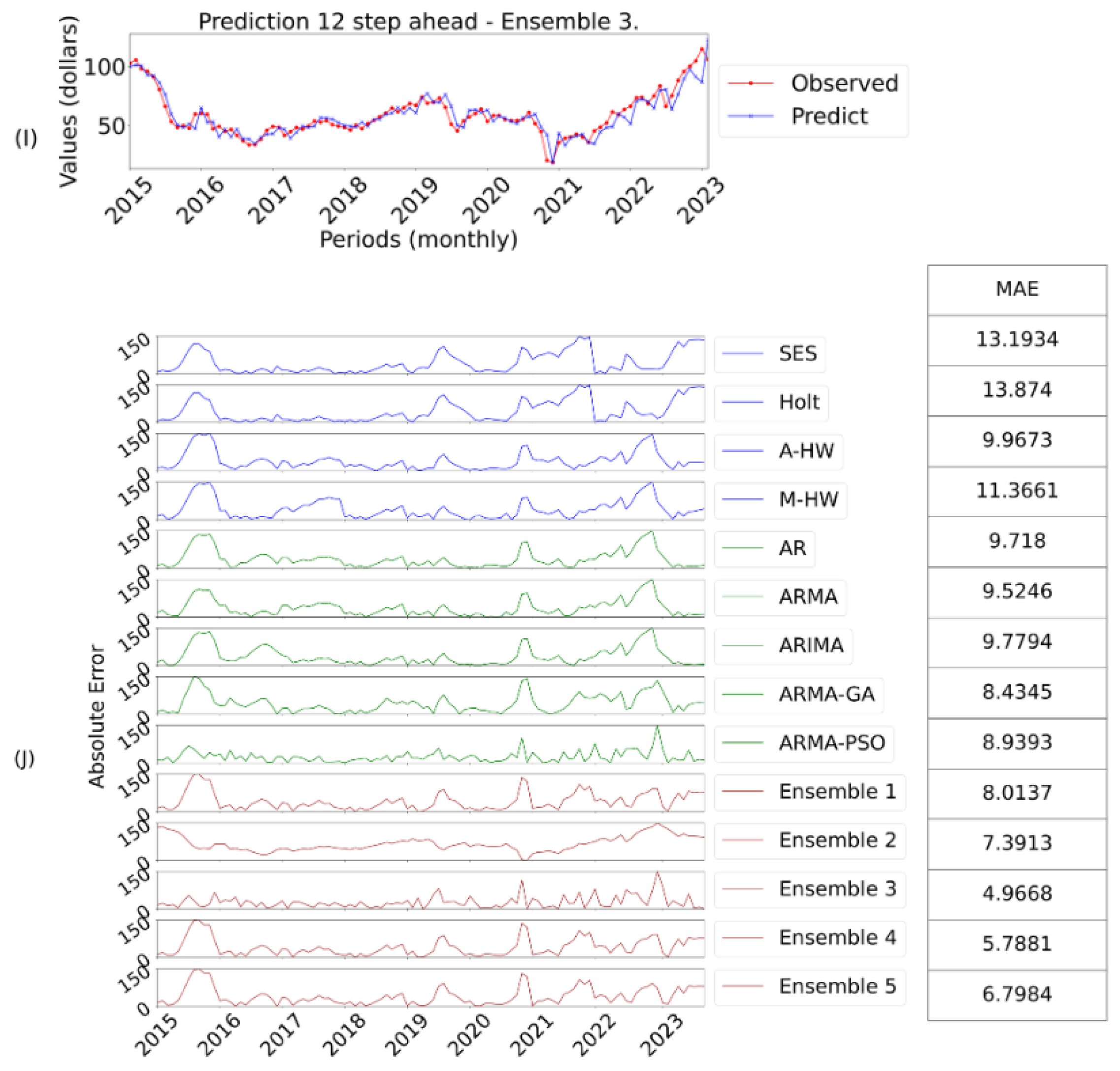
  • Figure 10: I contains the prediction of the best model and J the AE evaluation of the absolute error considering twelve-steps ahead.
As shown in Table 8, ensemble 5, using the weighted average with PSO, stood out by dynamically adjusting the weights of the models in the Ensemble based on historical performance, maximizing overall accuracy. This flexibility justifies its superior performance compared to ensembles 1 and 2, which assign equal weights to each model, according to Equations (17) and (18). By looking at the scores assigned to each model according to its performance per evaluation metric, it is possible to construct a score with the sum of all the scores. It can be seen that although ensemble 5 had the best overall performance, ensemble 3 stood out with the best position in relation to MAPE error.
Figure 6 illustrates the best model for predicting a step forward on the test set (Observed).
Subfigure A contains the predicted values with the best model. While subfigure B presents the absolute error for each predicted value of all models. Next to it are the values with the MAE errors per model. This analogy is used for the other predicted steps.
After evaluating the one-step ahead forecasts, we moved on to analyze the three-steps ahead horizons. Table 9 shows the results of all the models based on the MSE, MAE and MAPE error metrics.
For this horizon, ensemble 3 stood out, using the pseudo-inverse of Moore-Penrose to combine the models, taking better advantage of their individual characteristics. The ensembles 4 and 5 also outperformed the individual models, indicating the effectiveness of the GA and PSO approaches. Individual models such as AR, ARMA and ARIMA showed relatively high errors, with the multiplicative Holt Winters model obtaining the highest MSE.
In the three-steps horizon, the ARMA-GA model outperformed ARMA-PSO, possibly due to uncertainties in the parameter selection process. The smoothing models behaved similarly to the one-step horizon, with larger errors in multi-step forecasts. Ensemble 3 again stood out in this horizon.
As mentioned above and illustrated in Table 9, ensemble 3 obtained better results than all the predictive models. This is because ensemble 3 is more precise when adjusting the weights, directly minimizing the prediction error. In this case, it provides more sensitive and accurate responses to fluctuations, which are more evident in forecasts with longer horizons. Its performance is also evident when evaluating the final ranking, thus obtaining a better score in all error metrics. It is worth noting, however, that as in the previous step, ensembles 4 and 5 obtained good results compared to the other ensembles, again highlighting the efficiency of using GA and PSO. In this sense, Figure 7 shows the best prediction model, obtained by ensemble 3.
Similarly, we went on to evaluate other forecast horizons, in this case for six-steps ahead, as shown in Table 10.
Ensemble 3 was again superior, reinforcing its ability to determine the best weightings for longer forecasts. The ensemble 5 also stood out, showing the efficiency of the optimization algorithms. Its performance is also evident when evaluating the final ranking, thus obtaining a better score in all the error metrics. Ensemble 2, which uses the median, performed reasonably well, being robust against outliers as the steps increase. Figure 8 shows the best result for this horizon, obtained by ensemble 3.
After these considerations, the forecasts for the models considering nine-steps ahead were evaluated, as illustrated in Table 11.
Ensemble 3 stood out again, as shown in Table 11. As the horizons increase, the errors of the individual models increase significantly, which does not occur in the ensembles. Ensemble 3 was the best for forecasts nine-steps ahead, as illustrated in Figure 9. Its performance is also evident when evaluating the final ranking, thus obtaining a better score in all the error metrics. The Box & Jenkins models maintained their performance, highlighting the efficiency of the GA and PSO algorithms. Although ensemble 2 was not the best, it obtained considerable results, demonstrating its robustness for longer horizon forecasts, due to the reduction in variability when using central values.
Finally, with regard to the last forecast horizon, considering twelve-steps ahead, Table 12 shows the results of all the models.
The Box & Jenkins models maintained the same results as the previous cases. In the Smoothing models, there was a change, with the additive and multiplicative models, previously the worst, becoming the best. The ensemble 3 remains the most effective.
The exponential smoothing models showed variations in results, with the Additive Holt Winters being the most effective, especially in long-term forecasts, due to its stability and predictability. The SES model also benefited from stationarity in shorter horizon forecasts.
Finally, the results reinforce that ensemble 3 significantly outperformed the individual models, and the ensembles in general proved superior at other forecast horizons.
After the aforementioned considerations for a forecast horizon of twelve-steps ahead, Figure 10 shows the best answer, in this case ensemble 3.
Several were analyzed and MSE, MAE and MAPE were used to evaluate them. These metrics illustrate average values (the best overall approximation in the analysis). Abrupt changes in the direction of the time series make it difficult for models to predict, but some models have the ability to adapt better than others. By analyzing AE, it is possible to see which models have the smallest outliers, which is additional behavioral information that the usual averages do not provide.
The results presented in this section confirm the concepts discussed in the Section 2.4, demonstrating the robustness of the ensemble models over different forecast horizons. Specifically, ensemble 5 proved to be superior in the forecast horizon of one-step ahead, while for forecasts of 3, 6, 9 and 12 steps ahead, ensemble 3 was superior to all models.
In general, ensemble models have different advantages and disadvantages. The mean is simple, but can be influenced by outliers. The median is robust against outliers, but can ignore variability. The Moore-Penrose inverse optimizes weights based on historical performance, and is accurate but computationally complex. Weighted averaging with PSO and GA dynamically adjusts the weights, improving accuracy, but requires more computing power. For short-term forecasts, the mean and median are effective; for the long term, the inverse of Moore-Penrose and the weighted mean offer better optimization, provided there is sufficient data.

5. Conclusions

The main contribution of this work is related to the use of the pseudo-inverse of Moore-Penrose to determine the weights of the models to be used in the formation of the Ensemble, in addition to the use of metaheuristics.
It is known that GA and PSO algorithms are widely used in the literature, although not so much for application in ensemble. In this sense, as an initial work, it was decided to use these techniques.
The results show that the ensemble models, especially those that used metaheuristics and the pseudo-inverse of Moore-Penrose, significantly improved the individual results of the predictive models at all forecast horizons.
After pre-processing the data, the model parameters were determined in various ways: for the smoothing models, a numerical model that minimizes the cost function was used; for the Box & Jenkins models, the Yule-Walker equations and maximum likelihood estimators were used, with delays tested exhaustively. Specifically for the ARMA model, two coefficient optimization techniques were used: GA and PSO. For the ensemble, several strategies were tested, including arithmetic mean, median, pseudo-inverse of Moore-Penrose and weighted mean with GA and PSO. The results showed that the ensemble approaches outperformed the individual models, with the weighted average with PSO (ensemble 5) standing out in step 1, and the pseudo-inverse of Moore-Penrose (ensemble 3) in the other steps.
The results indicate the feasibility of using ensembles in time series forecasting, allowing it to be applied to forecasting models other than linear ones.
In this sense, the research can be further developed with the insertion of other approaches aimed at technological development, such as the creation of other Ensembles. Mention could be made of the use of artificial neural networks to form a non-linear ensemble.

Author Contributions

Conceptualization, J.L.F.d.S., Y.R.K., S.L.S.J. and H.V.S.; methodology, J.L.F.d.S., Y.R.K., S.L.S.J. and H.V.S.; software, J.L.F.d.S.; validation, J.L.F.d.S., Y.R.K., S.L.S.J., T.A.A. and H.V.S.; formal analysis, A.J.C.V.; investigation, J.L.F.d.S., Y.R.K. and H.V.S.; resources, T.A.A.; data curation, J.L.F.d.S., Y.R.K., S.L.S.J. and H.V.S.; writing—original draft preparation, J.L.F.d.S., Y.R.K., S.L.S.J. and H.V.S.; writing—review and editing, J.L.F.d.S., A.J.C.V., S.L.S.J. and H.V.S.; visualization, J.L.F.d.S.; supervision, H.V.S.; project administration, H.V.S.; funding acquisition, T.A.A. All authors have read and agreed to the published version of the manuscript.

Funding

This study was financed in part by the Coordenação de Aperfeiçoamento de Pessoa de Nível Superior—Brasil (CAPES)—Finance Code 001. The authors thank the Brazilian National Council for Scientific and Technological Development (CNPq), process numbers 315298/2020-0, 306448/2021-1, and 312367/2022-8, and Araucária Foundation, process number 51497 and 19.311.894-1, for their financial support.

Data Availability Statement

Data are contained within the article.

Conflicts of Interest

The authors declare no conflicts of interest.

Abbreviations

The following abbreviations are used in this manuscript:
ACFAutocorrelation function
AEAbsolute error
A-HWAdditive Holt-Winters’ models
ARAutoregressive
ARIMAAutoregressive integrated moving average
ARMAAutoregressive-moving-average
EIAEnergy Information administration
GAGenetic algorithm
HESHolt simple exponential smoothing
MAEMean absolute error
MAPEMean absolute percentage error
M-HWMultiplicative Holt-Winters’ models
MSEMean Squared Error
PACFPartial autocorrelation function
PSOParticle swarm optimization
SESSimple exponential smoothing
WTIWest Texas Intermediate

Appendix A

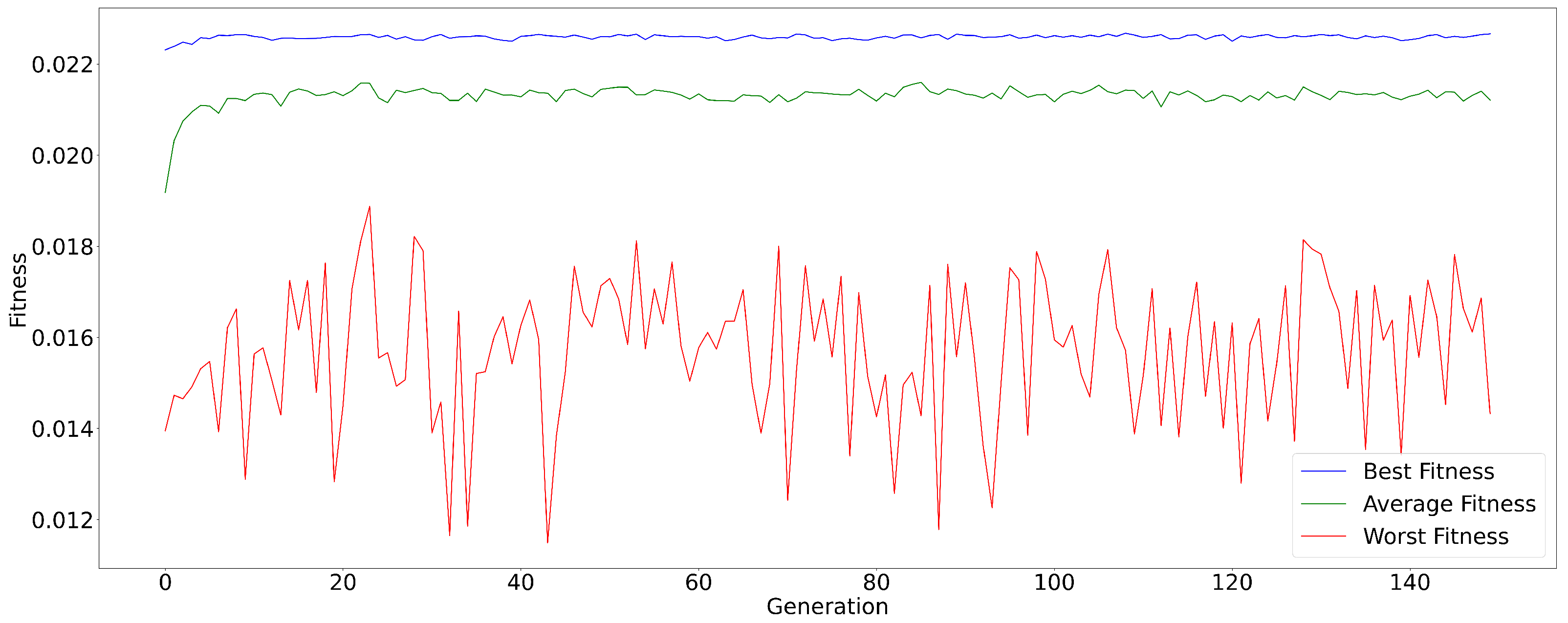
Together with the parameters observed in Table 3, the fitness of the adjusted model can be seen in Figure A1.
Figure A1. Fitness of the ARMA-A Model.
Energies 17 04058 g0a1
For the application of the Autoregressive Moving Average Model-ARMA( p , q ) with corrections using the PSO as mentioned in Section 3.4, the parameters used are shown in Table 4.
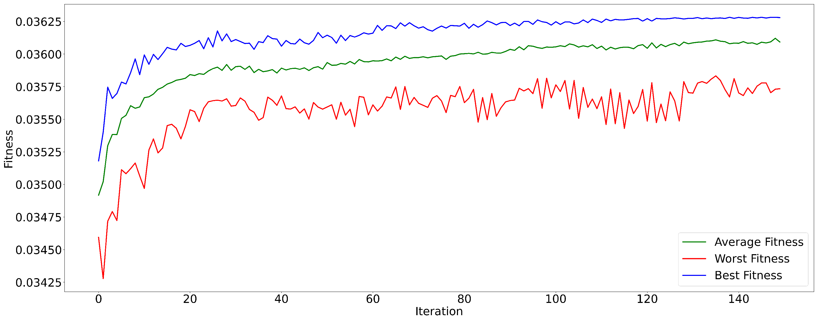
With the parameters observed in Table 4, the fitness of the adjusted model can be seen in Figure A2.
Figure A2. Fitness of the ARMA-PSO Model.
Energies 17 04058 g0a2
Adjustments of the ϕ and θ values with Table 5.
Table A1 shows the weights associated with the ensemble 3 model.
Table A1. Weights Associated with Ensemble 3.
ModelsWeights
SES5.3110
ARMA0.3103
AR0.9854
ARMA-PSO−0.0534
A-HW0.6266
M-HW−1.0575
HOLT−4.8867
ARIMA−1.1908
ARIMA-GA0.6770
Figure A3. Fitness of the Ensemble 4—GA Model.
Energies 17 04058 g0a3
Figure A4. Fitness of the Ensemble 5—PSO Model.
Energies 17 04058 g0a4
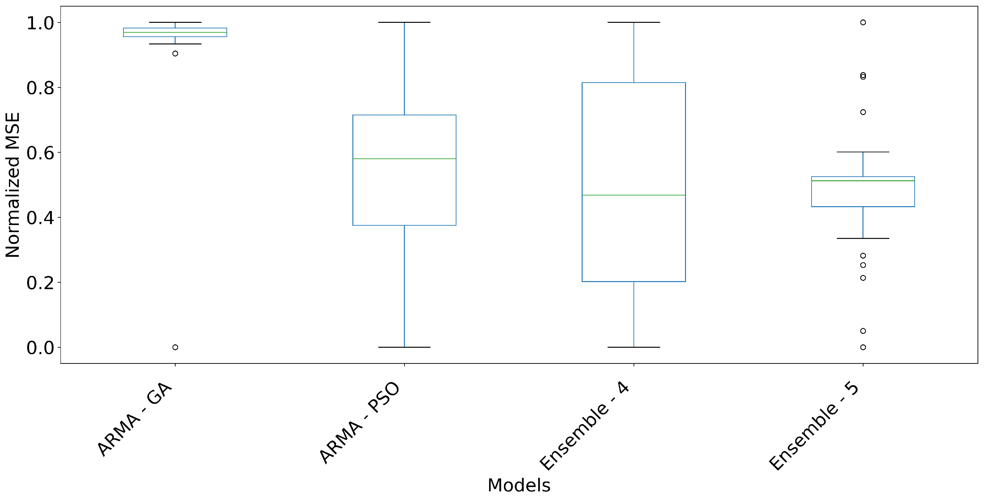
Figure A5. Model Dispersion.
Energies 17 04058 g0a5

References

  1. Administration, U.E.I. Petroleum & Other Liquids. 2023. Available online: https://www.eia.gov/petroleum (accessed on 3 June 2023).
  2. Duan, K.; Ren, X.; Wen, F.; Chen, J. Evolution of the information transmission between Chinese and international oil markets: A quantile-based framework. J. Commod. Mark. 2023, 29, 100304. [Google Scholar] [CrossRef]
  3. Balcilar, M.; Gabauer, D.; Umar, Z. Crude Oil futures contracts and commodity markets: New evidence from a TVP-VAR extended joint connectedness approach. Resour. Policy 2021, 73, 102219. [Google Scholar] [CrossRef]
  4. Lyu, Y.; Tuo, S.; Wei, Y.; Yang, M. Time-varying effects of global economic policy uncertainty shocks on crude oil price volatility: New evidence. Resour. Policy 2021, 70, 101943. [Google Scholar] [CrossRef]
  5. Khan, K.; Su, C.W.; Umar, M.; Yue, X.G. Do crude oil price bubbles occur? Resour. Policy 2021, 71, 101936. [Google Scholar] [CrossRef]
  6. Wang, X.; Li, X.; Li, S. Point and interval forecasting system for crude oil price based on complete ensemble extreme-point symmetric mode decomposition with adaptive noise and intelligent optimization algorithm. Resour. Policy 2022, 328, 120194. [Google Scholar] [CrossRef]
  7. Karasu, S.; Altan, A. Crude oil time series prediction model based on LSTM network with chaotic Henry gas solubility optimization. Energy 2022, 242, 122964. [Google Scholar] [CrossRef]
  8. Ren, X.; Liu, Z.; Jin, C.; Lin, R. Oil price uncertainty and enterprise total factor productivity: Evidence from China. Int. Rev. Econ. Financ. 2023, 83, 201–218. [Google Scholar] [CrossRef]
  9. Yuan, J.; Li, J.; Hao, J. A dynamic clustering ensemble learning approach for crude oil price forecasting. Eng. Appl. Artif. Intell. 2023, 123, 106408. [Google Scholar] [CrossRef]
  10. Zhang, T.; Tang, Z. The dependence and risk spillover between economic uncertainties and the crude oil market: New evidence from a Copula-CoVaR approach incorporating the decomposition technique. Environ. Sci. Pollut. Res. 2023, 83, 104116–104134. [Google Scholar] [CrossRef]
  11. Inacio, C.; Kristoufek, L.; David, S. Assessing the impact of the Russia—Ukraine war on energy prices: A dynamic cross-correlation analysis. Phys. A Stat. Mech. Its Appl. 2023, 626, 129084. [Google Scholar] [CrossRef]
  12. An, S.; An, F.; Gao, X.; Wang, A. Early warning of critical transitions in crude oil price. Energy 2023, 280, 128089. [Google Scholar] [CrossRef]
  13. Siqueira, H.; Boccato, L.; Attux, R.; Lyra, C. Unorganized machines for seasonal streamflow series forecasting. Int. J. Neural Syst. 2014, 24, 1299–1316. [Google Scholar] [CrossRef] [PubMed]
  14. Siqueira, H.; Belotti, J.T.; Boccato, L.; Luna, I.; Attux, R.; Lyra, C. Recursive linear models optimized by bioinspired metaheuristics to streamflow time series prediction. Int. Trans. Oper. Res. 2023, 30, 742–773. [Google Scholar] [CrossRef]
  15. Ren, Y.; Zhang, L.; Suganthan, P. Ensemble Classification and Regression-Recent Developments, Applications and Future Directions (Review Article). IEEE Comput. Intell. Mag. 2016, 11, 41–53. [Google Scholar] [CrossRef]
  16. Yu, L.; Xu, H.; Tang, L. LSSVR ensemble learning with uncertain parameters for crude oil price forecasting. Appl. Soft Comput. 2017, 56, 692–701. [Google Scholar] [CrossRef]
  17. Fathalla, A.; Alameer, Z.; Abbas, M.; Ali, A. A Deep Learning Ensemble Method for Forecasting Daily Crude Oil Price Based on Snapshot Ensemble of Transformer Model. Comput. Syst. Sci. Eng. 2023, 46, 929–950. [Google Scholar] [CrossRef]
  18. Cen, Z.; Wang, J. Crude oil price prediction model with long short term memory deep learning based on prior knowledge data transfer. Energy 2017, 169, 160–171. [Google Scholar] [CrossRef]
  19. Wang, M.; Tian, L.; Zhou, P. A novel approach for oil price forecasting based on data fluctuation network. Energy Econ. 2018, 71, 201–212. [Google Scholar] [CrossRef]
  20. Bildirici, M.; Bayazit, N.G.; Yasemen, U. Analyzing crude oil prices under the impact of COVID-19 by using lstargarchlstm. Energies 2020, 13, 2980. [Google Scholar] [CrossRef]
  21. Bekiroglu, K.; Duru, O.; Gulay, E.; Su, R.; Lagoa, C. Predictive analytics of crude oil prices by utilizing the intelligent model search engine. Appl. Energy 2018, 228, 2387–2397. [Google Scholar] [CrossRef]
  22. Gardner, E.S. Exponential smoothing: The state of the art—Part II. Int. J. Forecast. 2006, 22, 637–666. [Google Scholar] [CrossRef]
  23. Saputra, N.D.; Aziz, A.; Harjito, B. Parameter optimization of Brown’s and Holt’s double exponential smoothing using golden section method for predicting Indonesian Crude Oil Price (ICP). In Proceedings of the 2016 3rd International Conference on Information Technology, Computer, and Electrical Engineering (ICITACEE), Semarang, Indonesia, 19–20 October 2016; pp. 356–360. [Google Scholar] [CrossRef]
  24. Hyndman, R.J.; Khandakar, Y. Automatic Time Series Forecasting: The forecast Package for R. J. Stat. Softw. 2008, 27, 1–22. [Google Scholar] [CrossRef]
  25. Hyndman, R.J.; Athanasopoulos, G. Forecasting Principles and Practice; OTexts: Melbourne, Australia, 2021; Volume 3, pp. 1–442. [Google Scholar]
  26. Awajan, A.M.; Ismail, M.T.; Al Wadi, S. Improving forecasting accuracy for stock market data using EMD-HW bagging. PLoS ONE 2018, 13, 199582. [Google Scholar] [CrossRef]
  27. Papastefanopoulos, V.; Linardatos, P.; Kotsiantis, S. COVID-19: A Comparison of Time Series Methods to Forecast Percentage of Active Cases per Population. Appl. Sci. 2020, 10, 3880. [Google Scholar] [CrossRef]
  28. Box, G.; Jenkis, G.; Reinsel, C.; Ljung, M. Time series analysis: Forecasting and control. Wiley Ser. Probab. Stat. N. J. 2015, 301, 1–709. [Google Scholar]
  29. Theerthagiri, P.; Ruby, A.U. Seasonal learning based ARIMA algorithm for prediction of Brent oil Price trends. Multimed. Tools Appl. 2023, 18, 2485–24504. [Google Scholar] [CrossRef]
  30. Gujarati, D.N.; Porter, D.C. Econometria Básica-5; Amgh Editora: Porto Alegre, Brazil, 2011. [Google Scholar]
  31. Haykin, S. Adaptive Filter Theory; Pearson Education India: Chennai, India, 2002. [Google Scholar]
  32. Shadab, T.; Ahmad, S.; Said, S. Spatial forecasting of solar radiation using ARIMA model. Remote Sens. Appl. Soc. Environ. 2023, 20, 100427. [Google Scholar] [CrossRef]
  33. Almasarweh, M.; Wadi, S.A. ARIMA Model in Predicting Banking Stock Market Data. Mod. Appl. Sci. 2018, 12, 309–312. [Google Scholar] [CrossRef]
  34. Zhong, C. Oracle-efficient estimation and trend inference in non-stationary time series with trend and heteroscedastic ARMA error. Comput. Stat. Data Anal. 2024, 193, e1475. [Google Scholar] [CrossRef]
  35. Kennedy, J.; Eberhart, R. Particle swarm optimization. In Proceedings of the Proceedings of ICNN’95—International Conference on Neural Networks, Perth, WA, Australia, 27 November–1 December 1995; Bastos Filho, C.J.A., Pozo, A.R., Lopes, H.S., Eds.; IEEE: New York, NY, USA, 1995; Volume 4, pp. 1942–1948. [Google Scholar] [CrossRef]
  36. Cortez, P.; Rocha, M.; Neves, J. Evolving Time Series Forecasting ARMA Models. J. Heuristics 2012, 10, 137–151. [Google Scholar] [CrossRef]
  37. Binitha, S.; Sathya, S.S. A survey of bio inspired optimization algorithms. Int. J. Soft Comput. Eng. 2012, 2, 137–151. [Google Scholar]
  38. Holland, J.H. Adaptation in Natural and Artificial Systems: An Introductory Analysis with Applications to Biology, Control, and Artificial Intelligence; MIT Press: Cambridge, MA, USA, 1975. [Google Scholar]
  39. Goldberg, D. Genetic Algorithms in Search, Optimization, and Machine Learning; Addison-Wesley Publishing Company: London, UK, 1989. [Google Scholar]
  40. Michalewicz, Z.; Schoenauer, M. Evolving Time Series Forecasting ARMA Models. Evol. Comput. 1996, 4, 1–32. [Google Scholar] [CrossRef]
  41. Eren, B.; Rezan, U.V.; Ufuk, Y.; Erol, E. A modified genetic algorithm for forecasting fuzzy time series. Appl. Intell. 2014, 41, 453–463. [Google Scholar] [CrossRef]
  42. Aljamaan, I.; Alenany, A. Identification of Wiener Box-Jenkins Model for Anesthesia Using Particle Swarm Optimization. Appl. Sci. 2022, 12, 4817. [Google Scholar] [CrossRef]
  43. Edalatpanah, S.A.; Hassani, F.S.; Smarandache, F.; Sorourkhah, A.; Pamucar, D.; Cui, B. A hybrid time series forecasting method based on neutrosophic logic with applications in financial issues. Eng. Appl. Artif. Intell. 2024, 129, 107531. [Google Scholar] [CrossRef]
  44. Kennedy, J.; Eberhart, R.; Shi, Y. Swarm Intelligence; Evolutionary Computation Series; Elsevier Science: Amsterdam, The Netherlands, 2001. [Google Scholar]
  45. Donate, J.P.; Cortez, P.; Sánchez, G.G.; de Miguel, A.S. Time series forecasting using a weighted cross-validation evolutionary artificial neural network ensemble. Neurocomputing 2013, 109, 27–32. [Google Scholar] [CrossRef]
  46. Silva, E.G.; de O. Júunior, D.S.; Cavalcanti,, G.D.C.; de Mattos Neto, P.S.G. Improving the accuracy of intelligent forecasting models using the Perturbation Theory. In Proceedings of the 2018 International Joint Conference on Neural Networks (IJCNN), Rio de Janeiro, Brazil, 8–13 July 2018; IEEE: New York, NY, USA, 2018; pp. 1–7. [Google Scholar] [CrossRef]
  47. Wang, L.; Wang, Z.; Qu, H.; Liu, S. Optimal Forecast Combination Based on Neural Networks for Time Series Forecasting. Appl. Soft Comput. 2018, 66, 1–17. [Google Scholar] [CrossRef]
  48. Perrone, M.P.; Cooper, L. When Networks Disagree: Ensemble Methods for Hybrid Neural Networks; World Scientific Publishing: Singapore, 1995; Volume 109, pp. 1–404. [Google Scholar]
  49. Sun, Y.; Tang, K.; Zhu, Z.; Yao, X. Concept Drift Adaptation by Exploiting Historical Knowledge. IEEE Trans. Neural Netw. Learn. Syst. 2018, 29, 4822–4832. [Google Scholar] [CrossRef] [PubMed]
  50. Britto, A.S.; Sabourin, R.; Oliveira, L.E. Dynamic selection of classifiers—A comprehensive review. Pattern Recognit. 2014, 47, 3665–3680. [Google Scholar] [CrossRef]
  51. Nosrati, V.; Rahmani, M. An ensemble framework for microarray data classification based on feature subspace partitioning. Comput. Biol. Med. 2022, 148, 105820. [Google Scholar] [CrossRef]
  52. Wilson, J.; Chaudhury, S.; Lall, B. Homogeneous—Heterogeneous Hybrid Ensemble for concept-drift adaptation. Neurocomputing 2023, 557, 126741. [Google Scholar] [CrossRef]
  53. Mendes-Moreira, J.A.; Soares, C.; Jorge, A.M.; Sousa, J.F.D. Ensemble approaches for regression: A survey. ACM Comput. Surv. 2012, 45, 1–40. [Google Scholar] [CrossRef]
  54. Heinermann, J.; Kramer, O. Machine learning ensembles for wind power prediction. Renew. Energy 2016, 89, 671–679. [Google Scholar] [CrossRef]
  55. Ma, Z.; Dai, Q. Selected an Stacking ELMs for Time Series Prediction. Neural Process. Lett. 2016, 44, 831–856. [Google Scholar] [CrossRef]
  56. de Oliveira, J.F.L.; Silva, E.G.; de Mattos Neto, P.S.G. A Hybrid System Based on Dynamic Selection for Time Series Forecasting. IEEE Trans. Neural Netw. Learn. Syst. 2022, 33, 3251–3263. [Google Scholar] [CrossRef] [PubMed]
  57. Cruz, R.M.; Sabourin, R.; Cavalcanti, G.D. Dynamic classifier selection: Recent advances and perspectives. Inf. Fusion 2018, 41, 195–216. [Google Scholar] [CrossRef]
  58. Barrow, D.K.; Crone, S.F.; Kourentzes, N. An evaluation of neural network ensembles and model selection for time series prediction. In Proceedings of the the 2010 International Joint Conference on Neural Networks IJCNN, Barcelona, Spain, 18–23 July 2010; IEEE: New York, NY, USA, 2010; pp. 1–8. [Google Scholar] [CrossRef]
  59. Kourentzes, N.; Barrow, D.K.; Crone, S.F. Neural network ensemble operators for time series forecasting. Expert Syst. Appl. 2014, 41, 4235–4244. [Google Scholar] [CrossRef]
  60. Kazmaier, J.; van Vuuren, J.H. The power of ensemble learning in sentiment analysis. Expert Syst. Appl. 2022, 187, 115819. [Google Scholar] [CrossRef]
  61. Chung, D.; Yun, J.; Lee, J.; Jeon, Y. Predictive model of employee attrition based on stacking ensemble learning. Expert Syst. Appl. 2023, 215, 119364. [Google Scholar] [CrossRef]
  62. Kuncheva, L.I.; Rodríguez, J.J. A weighted voting framework for classifiers ensembles. Knowl. Inf. Syst. 2014, 38, 259–275. [Google Scholar] [CrossRef]
  63. Large, J.; Lines, J.; Bagnall, A. A probabilistic classifier ensemble weighting scheme based on cross-validated accuracy estimates. Data Min. Knowl. Discov. 2019, 33, 1674–1709. [Google Scholar] [CrossRef]
  64. Baradaran, R.; Amirkhani, H. Ensemble learning-based approach for improving generalization capability of machine reading comprehension systems. Neurocomputing 2021, 33, 229–242. [Google Scholar] [CrossRef]
  65. Baksalary, O.M.; Trenkler, G. The Moore–Penrose inverse: A hundred years on a frontline of physics research. Eur. Phys. J. H 2021, 46, 9. [Google Scholar] [CrossRef]
  66. Safari, A.; Davallou, M. Oil price forecasting using a hybrid model. Energy 2018, 148, 49–58. [Google Scholar] [CrossRef]
  67. Cox, D.R.; Stuart, A. Some quick sign tests for trend in location and dispersion. Biometrika 1955, 42, 80–95. [Google Scholar] [CrossRef]
  68. Sprent, P.; Smeeton, N.C. Applied Nonparametric Statistical Methods; CRC Press: Boca Raton, FL, USA, 2016. [Google Scholar]
  69. Chyon, F.A.; Suman, M.N.H.; Fahim, M.R.I.; Ahmmed, M.S. Time series analysis and predicting COVID-19 affected patients by ARIMA model using machine learning. J. Virol. Methods 2022, 301, 114433. [Google Scholar] [CrossRef] [PubMed]
  70. Montgomery, D.; Jennings, C.L.; Kulachi, M. Introduction to Time Series Analysis and Forecasting; John Wiley & Sons: Cambridge, MA, USA, 2008. [Google Scholar]
  71. Siqueira, H.V.; Luna, I. Modelos Lineares Realimentados de Previsão: Um Estudo Utilizando Algoritmos Evoluciionários. In Proceedings of the Anais do 12 Congresso Brasileiro de Inteligência Computacional, Curitiba, Brazil, 13–16 October 2016; Bastos Filho, C.J.A., Pozo, A.R., Lopes, H.S., Eds.; pp. 1–6. [Google Scholar]
  72. Awan, T.M.; Aslam, F. Prediction of daily COVID-19 cases in European countries using automatic ARIMA model. J. Public Health Res. 2021, 9, 4101–4111. [Google Scholar] [CrossRef]
  73. Alsharef, A.; Aggarwal, K.; Sonia; Kumar, M.; Mishra, A. Review of ML and AutoML Solutions to Forecast Time-Series Data. Arch. Comput. Methods Eng. 2022, 46, 5297–5311. [Google Scholar] [CrossRef] [PubMed]
  74. Ubaid, A.; Hussain, F.; Saqib, M. Container Shipment Demand Forecasting in the Australian Shipping Industry: A Case Study of Asia—Oceania Trade Lane. J. Mar. Sci. Eng. 2021, 9, 968. [Google Scholar] [CrossRef]
Figure 1. Non-trainable Ensemble Flowchart.
Energies 17 04058 g001
Figure 2. Trainable Ensemble Flowchart.
Energies 17 04058 g002
Figure 3. Stages for Forecasts with Linear Models and Ensemble.
Energies 17 04058 g003
Figure 4. WTI Crude Oil Price.
Energies 17 04058 g004
Figure 5. Autocorrelation and Partial Autocorrelation.
Energies 17 04058 g005
Figure 6. Ensemble 5 Forecasts One-Step Ahead and Errors.
Energies 17 04058 g006
Figure 7. Ensemble 3 Forecasts Three-Steps Ahead and Errors.
Energies 17 04058 g007
Figure 8. Ensemble 3 Forecasts Six-Steps Ahead and Errors.
Energies 17 04058 g008
Figure 9. Ensemble 3 Forecasts Nine-Steps Ahead and Errors.
Energies 17 04058 g009
Figure 10. Ensemble 3 Forecasts Twelve-Steps Ahead and Errors.
Energies 17 04058 g010
Table 1. Smoothing Model Coefficients.
Models α β γ
SES1.00--
Holt1.00 1.09 × 10 4 -
A-HW 9.99 × 10 3 4.65 × 10 8 3.17 × 10 8
M-HW1.00 8.75 × 10 11 6.67 × 10 11
Source: Own authorship (2024).
Table 2. Box & Jenkins Model Coefficients.
Modelspdq
AR1--
ARMA1-3
ARIMA616
Source: Own authorship (2024).
Table 3. Description of GA Parameters—ARMA.
ParametersValues
Population Size50
Number of Iterations30
Offspring Generated by Crossover50
Mutation Amplitude Regulator0.1
Percentage Mutation Rate10 %
Frequency of Use of Local Search100
Local Search Delta0.05
Maximum Number of Generations150
Search Interval for ϕ [−1, 1]
Search Interval for θ [−1, 1]
Source: Own authorship (2024).
Table 4. Description of the PSO—ARMA Parameters.
ParametersValues
Number of Particles150
Number of Iterations150
Inertia Coefficient w0.7
Cognitive Term c 1 2.0
Social Term c 2 2.0
Maximum Number of Executions30
Local Search Delta0.05
Search Interval for ϕ [−1, 1]
Search Interval for θ [−1, 1]
Source: Own authorship (2024).
Table 5. ARMA ( p , q ) GA and PSO Model.
Model ϕ 1 Θ 1 Θ 2 Θ 3
ARMA-GA0.1192−0.0081−0.0586−0.1268
ARMA-PSO0.6036−0.55370.1161−0.0438
Source: Own authorship (2024).
Table 6. Description of the GA Parameters for Optimizing the Weights in a Weighted Average Ensemble.
ParametersValues
Population Size150
Number of Iterations30
Offspring Generated by CrossoverBy Generation, Half of the Population
Crossover Rate90%
Mutation Rate50%
Mutation Amplitude (Standard Deviation)0.1
Tournament Size4
Number of Individual Models9
Source: Own authorship (2024).
Table 7. Description of the PSO Parameters for Optimizing the Weights in a Weighted Average Ensemble.
ParametersValues
Number of Particles150
Number of Iterations150
Inertia Coefficient w0.9
Cognitive Term c 1 2.0
Social Term c 2 2.0
Maximum Number of Executions30
Number of Models by Particle9
Source: Own authorship (2024).
Table 8. Evaluation and Rankings for One-Step Ahead Forecasts.
ModelsMSEMAEMAPERank MSERank MAERank MAPETotal ScoreFinal Ranking
Ensemble 526.13243.80520.073211241
Ensemble 126.59793.88550.074823382
ARMA-PSO35.74614.54610.0836344113
ARMA-GA36.09044.57790.0845455144
SES39.32764.72440.0878588215
Holt39.73904.73830.0881699246
ARMA42.16664.96350.0917767207
ARIMA42.27074.98960.0915876218
AR42.56775.01390.092491110309
M-HW43.64465.07920.09311013123510
A-HW42.70635.04710.09401112133611
Ensemble 238.11034.83850.0888710112812
Ensemble 442.85945.02800.93891214144013
Ensemble 347.25203.83630.073214211714
Source: Own authorship (2024).
Table 9. Evaluation and Rankings for Three-Steps Ahead Forecasts.
ModelsMSEMAEMAPERank MSERank MAERank MAPETotal ScoreFinal Ranking
Ensemble 331.58564.26310.080911131
Ensemble 546.62885.11970.1039262102
ARMA-GA62.98344.57790.1230335113
ARMA-PSO72.12696.29790.1148443114
Ensemble 462.11476.02900.1206554145
SES85.83546.82820.1371686206
Holt87.44506.92250.1385797237
Ensemble 180.26166.61110.1325878238
ARMA93.72714.36980.1500929209
ARIMA94.13667.12620.14511010113110
AR97.72227.43930.15721111123411
A-HW100.03557.19510.14911212103412
M-HW105.92397.56850.15281313133913
Ensemble 2116.43338.16100.15401414144214
Source: Own authorship (2024).
Table 10. Evaluation and Rankings for Six-Steps Ahead Forecasts.
ModelsMSEMAEMAPERank MSERank MAERank MAPETotal ScoreFinal Ranking
Ensemble 336.68874.80880.094011131
Ensemble 442.23605.14210.098522262
Ensemble 570.88416.18350.118233393
Ensemble 292.17166.96100.1375444124
ARMA-PSO102.77937.64400.1418555155
ARMA-GA108.80527.98440.1469666186
Ensemble 1113.81137.73890.1515777217
SES145.37746.65410.171811810298
ARIMA143.95468.55160.16331097269
AR141.21048.60260.163391082710
ARMA136.26958.83490.165681192811
A-HW152.34478.81440.17341312123712
Holt151.83698.87010.17471213113613
M-HW181.01559.79330.18551414134114
Source: Own authorship (2024).
Table 11. Evaluation and Rankings for Nine-Steps Ahead Forecasts.
ModelsMSEMAEMAPERank MSERank MAERank MAPETotal ScoreFinal Ranking
Ensemble 340.79995.17850.099612251
Ensemble 442.87635.02180.094821142
Ensemble 576.22046.61190.121233393
Ensemble 2107.05547.72300.1550444124
ARMA-GA116.78208.25920.1580556165
ARMA-PSO138.90018.37520.1573665176
Ensemble 1131.76568.60140.1707777217
SES195.832510.27510.20501089278
ARMA183.863510.26830.1816898259
AR207.423810.76310.1998910102910
Holt209.916910.72950.21211111103211
ARIMA235.277211.77770.22301212113512
M-HW262.916912.35680.22531413123913
A-HW254.086612.46840.23571314134014
Source: Own authorship (2024).
Table 12. Evaluation and Rankings for Twelve-Steps Ahead Forecasts.
ModelsMSEMAEMAPERank MSERank MAERank MAPETotal ScoreFinal Ranking
Ensemble 342.3994.96680.098011131
Ensemble 459.78945.78810.110322262
Ensemble 584.68156.79840.128633393
Ensemble 2106.86667.39130.1541444124
ARMA-GA120.21888.43450.1550565165
Ensemble 1122.83968.01370.1633657186
ARMA-PSO147.16788.93930.1641776207
ARMA160.83679.52460.1768888248
AR179.39929.71800.1840999279
ARIMA191.23719.77940.18911010103010
A-HW190.49709.96730.19671111113311
M-HW238.742111.36610.21291212123612
SES346.111313.19340.24691313133913
Holt379.384113.87400.25701414144214
Source: Own authorship (2024).
Disclaimer/Publisher’s Note: The statements, opinions and data contained in all publications are solely those of the individual author(s) and contributor(s) and not of MDPI and/or the editor(s). MDPI and/or the editor(s) disclaim responsibility for any injury to people or property resulting from any ideas, methods, instructions or products referred to in the content.