Article

TransRUL: A Transformer-Based Multihead Attention Model for Enhanced Prediction of Battery Remaining Useful Life

1
School of Automation, Northwestern Polytechnical University, Xi’an 710072, China
2
College of Engineering and IT, University of Dubai, Dubai 14143, United Arab Emirates
3
Department of Electrical Engineering, The Islamia University of Bahawalpur, Bahawalpur 63100, Pakistan
*
Authors to whom correspondence should be addressed.
Energies 2024, 17(16), 3976; https://doi.org/10.3390/en17163976
Submission received: 6 July 2024 / Revised: 5 August 2024 / Accepted: 8 August 2024 / Published: 11 August 2024
(This article belongs to the Section F: Electrical Engineering)

Abstract

:
The efficient operation of power-electronic-based systems heavily relies on the reliability and longevity of battery-powered systems. An accurate prediction of the remaining useful life (RUL) of batteries is essential for their effective maintenance, reliability, and safety. However, traditional RUL prediction methods and deep learning-based approaches face challenges in managing battery degradation processes, such as achieving robust prediction performance, to ensure scalability and computational efficiency. There is a need to develop adaptable models that can generalize across different battery types that operate in diverse operational environments. To solve these issues, this research work proposes a TransRUL model to enhance battery RUL prediction. The proposed model incorporates advanced approaches of a time series transformer using a dual encoder with integration positional encoding and multi-head attention. This research utilized data collected by the Centre for Advanced Life Cycle Engineering (CALCE) on CS_2-type lithium-ion batteries that spanned four groups that used a sliding window technique to generate features and labels. The experimental results demonstrate that TransRUL obtained superior performance as compared with other methods in terms of the following evaluation metrics: mean absolute error (MAE), root-mean-squared error (RMSE), and R 2 values. The efficient computational power of the TransRUL model will facilitate the real-time prediction of the RUL, which is vital for power-electronic-based appliances. This research highlights the potential of the TransRUL model, which significantly enhances the accuracy of battery RUL prediction and additionally improves the management and control of battery-based systems.

1. Introduction

The recent advancements in electric vehicles and renewable energy storage applications have developed a significant demand for lithium-ion batteries (LIBs). LIBs are essential to many applications, including electric vehicles, aerospace systems, and portable devices. Due to the increasing demand for renewable energy sources, the demand for advanced predictive maintenance strategies for batteries is increasing since they are vital for safe operation [1]. As these batteries age, their material mechanisms interact with one another due to surface cracking, material dissolution, and the growth of a solid electrolyte inter-phase layer. Therefore, the LIB’s performance decreases, potentially causing safety and reliability issues [2]. The precise prediction of the RUL is particularly important for ensuring their reliability and safety during operation. An accurate prediction of a battery’s RUL can help with planning for predictive maintenance, preventing an unpredicted failure, and extending the useful life of the battery [3].
The conventional RUL prognosis techniques have primarily depended on physical modeling and basic statistical techniques, which often fail to capture the complex degradation procedures of the latest battery technologies. The conventional RUL prognosis methods usually include empirical models and statistical techniques by using Kalman filters, particle filters, and Bayesian approaches. These conventional methods typically require significant domain knowledge and are limited by their incapacity to operate according to the nonlinear and dynamic nature of battery aging [4]. The research work in [5] used a particle-filter-based framework for the modeling of LIBs’ capacity depletion and showed the ability of this technique in handling uncertainties in a battery degradation process.
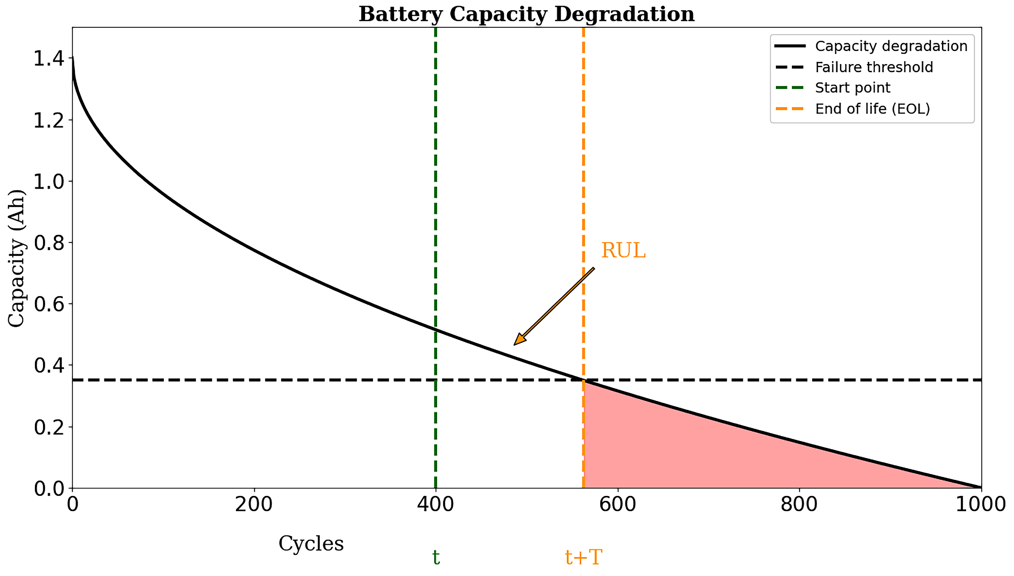
Figure 1 demonstrates the battery capacity degradation over multiple cycles to predict the RUL. The battery’s full capacity was 1.4 ampere hours (Ah); the failure threshold was 75 percent, which was at 0.35 Ah; and observation starting point was at 400 cycles. The capacity degradation curve crossed the threshold line at 562.5 cycles, which was the end of life (EOL) point, and thus, the RUL was the difference between the observation starting point to the EOL, which was 162 cycles. The shaded area from cycle 562.5 to 1000 suggests replacing the battery or improving its capacity through maintenance.
As long as batteries work under various operating conditions, the degradation patterns can be extremely nonlinear and affected by multiple factors, such as the temperature, discharge rates, and used cycles. This has led to the research of machine learning (ML) techniques that can learn these complex patterns from data.
The research work in [6] examined various methods that utilize ML and statistical-based models to forecast the RUL using historical recorded data. These methods include support vector machines (SVMs), random forests, gradient boosting machines, artificial neural networks (ANNs), convolution neural networks (CNNs), long short-term memory (LSTM), recurrent neural networks (RNNs), gated recurrent units (GRUs), attention-based models, and auto-encoders. However, these models often struggle with the complexity and nonlinearity of battery degradation processes. Contemporary research has developed many hybrid models that combine the traditional ML method with deep learning (DL) to improve the RUL prediction accuracy. The authors of [7] investigated and compared how well various DL-based hybrid models work. These include CNNs with wavelet packet decomposition and RNNs with nonlinear auto-regressive exogenous models. SVMs have been extensively utilized for fault classification [8] and RUL prediction due to their strong ability to handle high-dimensional data. However, the research work in [9], which compared an SVM with LSTM and GRU models, indicates that SVMs may not be as effective as DL models in capturing the complex, nonlinear relationships inherent in battery degradation data. ANNs were the first AI-based techniques to be used for RUL prognosis. The working principle of neural architecture is like a human brain’s ability to understand data and detect patterns. These methods are useful in applications in which the connection between the input data and the target cell is difficult and nonlinear. If not properly regularized, it can lead to over-fitting and requires significant computational resources for model training [10].
CNNs have achieved popularity for their strong ability to automatically capture features from unprocessed data for RUL prediction. A technique based on a deep dilated CNN (D-CNN) was proposed in [11] to enhance the receptive field and improve the prediction accuracy. This model presented good performance on the C-MAPSS dataset and required less training time compared with conventional methods. However, it required high computing power and skill to avoid over-fitting problems. Additionally, it had a lower prediction accuracy than the RNN and LSTM. RNNs are a type of neural network that can effectively model sequence data. RNNs developed from feed-forward networks behave like human brains. An RNN outperforms other algorithms at predicting sequential data [12]. LSTM networks are a variant of an RNN that can capture long-term dependencies in historical data of battery degradation for RUL prediction. It controls data flow in recurrent computations with gates. LSTM networks can hold long-term memories. Depending on the data, the network may or may not retain memory. The network’s gating mechanisms preserve long-term dependencies. The network may store or release memory through gating [13]. In the research work of [9], the LSTM-RNN method of RUL prediction was developed using six different cells from the NCR18650PF battery datasets. The RMS prop method was used to train on a combination of online and offline data for an LSTM-RNN model. The dropout technique was used to reduce over-fitting. The results indicate that the LSTM-RNN outperformed the SVM and a simple RNN. However, this model’s accuracy still needs to be improved and other batteries also need to test the model in the future.
An advanced framework for the RUL prediction of LIBs is presented in [14], where online real-world data and a NASA battery dataset were used. This method consists of three stages. First, using the state of charge equation, the value of the state of health (SOH) is predicted for each separate vehicle. In the second stage, the Lasso regression model was developed on aggregated data for all vehicles. Then, the internal and real battery parameters were predicted by using a Monte Carlo simulation method. In the last stage, the RUL was predicted through a probability distribution of SOH values using the Lasso model. This method works for both the short-term and long-term demands of electric-by-electric vehicles. However, the prediction error still needs to be reduced. In [15], a GRU-RNN model is proposed by using the adaptive gradient descent approach to enhance the RUL prediction accuracy and reduce the computing costs. The GRU-RNN model shows reliable performance through the experiments as compared with LSTM and an SVM, while having an average RMS error of around 2%. Another technique for RUL prediction is presented in [16], where it combines the Monte Carlo dropout and GRU to compensate for uncertainty in estimation results and prevent over-fitting. This technique provided probabilistic distribution-based RUL results that need to be improved. Attention mechanisms focus more on relevant features [17] and were recently incorporated into multiple DL-based models to enhance the prediction accuracy.
Attention techniques have enhanced IoT networks by increasing the network speed and security especially in unmanned aerial vehicle (UAV)-enabled networks. The research work in [18] presents an innovative UAV trajectory planning method that blends risk factor optimization with energy consumption and uses attention mechanisms to enhance the UAV’s real-time decision making in risky environments. Attention mechanisms filter and prioritize sensor data to focus on mission-critical information. UAVs can quickly make intelligent decisions based on the most relevant and current data because of their selective attention. By incorporating TinyML, the attention mechanisms deliver more decision-making privileges to the UAVs to independently conduct extensive computations and amendments. The research work [19] introduces a deep policy gradient action quantization (DPGAQ) technique that utilizes attention with deep reinforcement learning (DRL) to effectively manage the high-dimensional actions of vehicle networks. This work used attention processes that enable the DRL model to make quick decisions by focusing on the most important environmental features. This selectivity effectively controls the intelligent vehicle network’s high-dimensional data input issues. Attention techniques help the model control, and thus, minimize the number of unnecessary computations and enhance the rate of decisions and accuracy of actions to be taken. In [20], the authors developed a hybrid model by integrating a TCN, GRU, and deep neural network (DNN) by incorporating attention mechanisms. Initially, a TCN with a feature attention mechanism was used to capture the degradation patterns. Then, a combined TCN-GRU was used as a decoder to obtain a better understanding of data patterns using features, and finally, a DNN was used to predict the RUL through a multi-layer operation. The experimental work used the CALCE and NASA battery datasets to train and evaluate the model. However, this method needs high computational power and skill, and also needs to check the model on online data.
Transformer models are considered superior for predicting the RUL of LIBs due to their advanced capabilities. They apply self-attention mechanisms to effectively manage noisy data, capture complex dependencies, and also integrate denoising and prediction operations into a unified structure [21]. Transformers simultaneously process entire input sequences, leading to faster training and inference time compared with sequential models. Transformers are more efficient and effective than ANN, CNN, LSTM, RNN, GRU, and hybrid models. This is because the transformer benefits from transfer learning from the pre-trained model, which leads to better performance with less labeled data and a short training time [22]. To improve the prediction accuracy of the RUL for LIBs, the research work in [23] presents a transformer-based method that uses the capacity regeneration (CR) phenomenon. The increased value of CR leads to inaccuracies in RUL estimation. The first step is to pre-train the LSTM with the transformer-learning model without the CR of the NASA battery dataset. After pre-training, the weights of the first two layers are frozen. In the second step, the data are updated for training through the CR algorithm and the model is fine tuned with unfrozen layers. The results show that the mean relative error was 9%, which still needs to be improved. However, this model’s results fully depend on the efficiency of the CR algorithm.
The denoising encoder with a transformer-based framework developed in [24] by using the NASA battery datasets was further normalized and denoised by utilizing one-dimensional convolution layers to decrease the noise. The data patterns are captured using a transformer encoder. A multi-head self-attention mechanism and feed-forward network enhances the RUL prediction. This model can face difficulties for longer sequences of data because its flattening of the feature edges may not effectively capture sharp peaks or sudden data changes, which leads to inaccuracies. Furthermore, results need to be improved and validated across different batteries. Therefore, after critical analysis, it was found that DL-based methods struggle to effectively manage the complex and nonlinear degradation processes of LIB datasets, and their reliability under different operational conditions is challenging [25]. DL-based methods require significant computational power and skills and face over-fitting issues [26]. Current transformer-based methods involve flattening the feature edges since they cannot capture sharp peaks and they have computational complexity [27].
To address all the issues mentioned in this section, this research work proposes a TransRUL framework for the RUL prediction of LIBs, which was especially designed for time series data to enhance the capture of temporal dependencies. The TransRUL model uses a dual encoder and a self-attention mechanism to handle complex patterns of LIB datasets and integrates the embedding layers to convert data to a higher-dimensional vector space. It incorporates positional encoding for understanding the complex sequence’s temporal and multi-head attention to focus the input sequence simultaneously and enhance the overall model ability to capture complex dependencies, dropout layers to prevent over-fitting, and a transformer decoder layer to make accurate RUL predictions. This proposed TransRUL model will provide a robust framework for assessing a battery RUL, thus contributing valuable insights to the field of battery management systems. The principal contributions of this research are outlined as follows:
  • The proposed TransRUL model integrates the positional encoding and multi-head attention mechanisms with a dual encoder for capturing complex temporal dependencies in LIB datasets.
  • The model incorporates an advanced attention mechanism that selectively focuses on important features through temporal sequences, hence improving the RUL prediction accuracy.
  • The sliding-window-based technique is utilized in the TransRUL model to effectively capture temporal patterns in LIB data for generating feature–label pairs.
  • The inclusion of positional encoding and transformer encoder layers in the model strengthens the feature extraction without increasing the computing complexity.
  • A comprehensive set of evaluation metrics, including MAE, RMSE, and R2, were used to evaluate the overall performance of the proposed model with existing models, like CNN, LSTM, CNN-LSTM, CNN-Transformer, and latest research work.

2. Dataset and Evaluation Metrics

2.1. CALCE Capacity Dataset

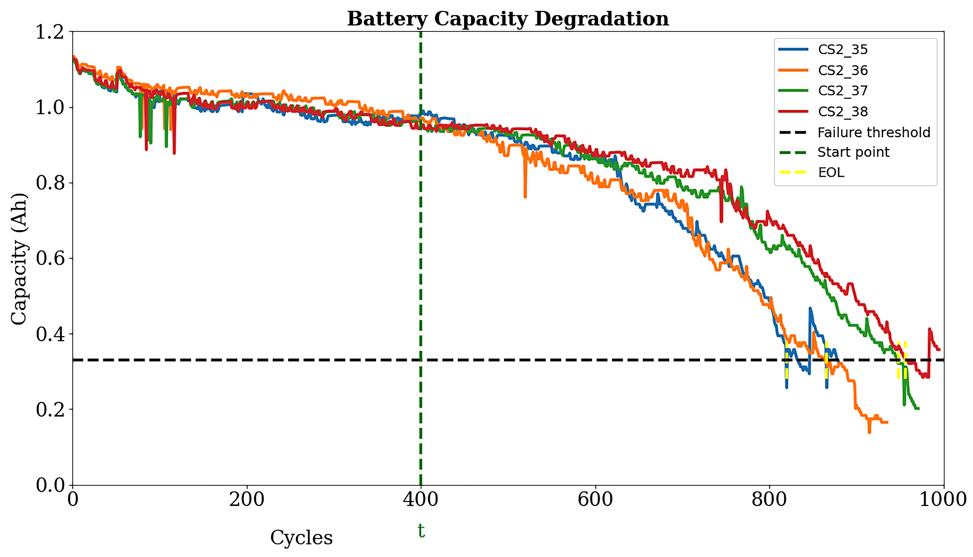
This work used the publicly available CALCE capacity dataset of four LIB batteries: C S _ 35 , C S _ 36 , C S _ 37 , and C S _ 38 . This dataset was published by the University of Maryland, and the standard capacity of each battery was 1.1 Ah. We used one leave-out-one-cross (LOOC) validation to train and test the model. Figure 2 shows the capacity curves of all batteries that were used to predict the RUL. Initially, the battery was charged through a constant current with a value of 1 A. If during charging, the current value was dropped to 0.5 A, then the charging model was switched to charge it through a constant voltage until it reached 4.2 V.
The environmental temperature was maintained at 25 °C during the charging and discharging process. The batteries were also discharged in continuous mode by a 1 A load until their voltages reached 2.7 V. When the battery’s initial capacity of 1.1 Ah reduced to 30% of its value (0.77 Ah), it was considered as the battery’s end of useful life.
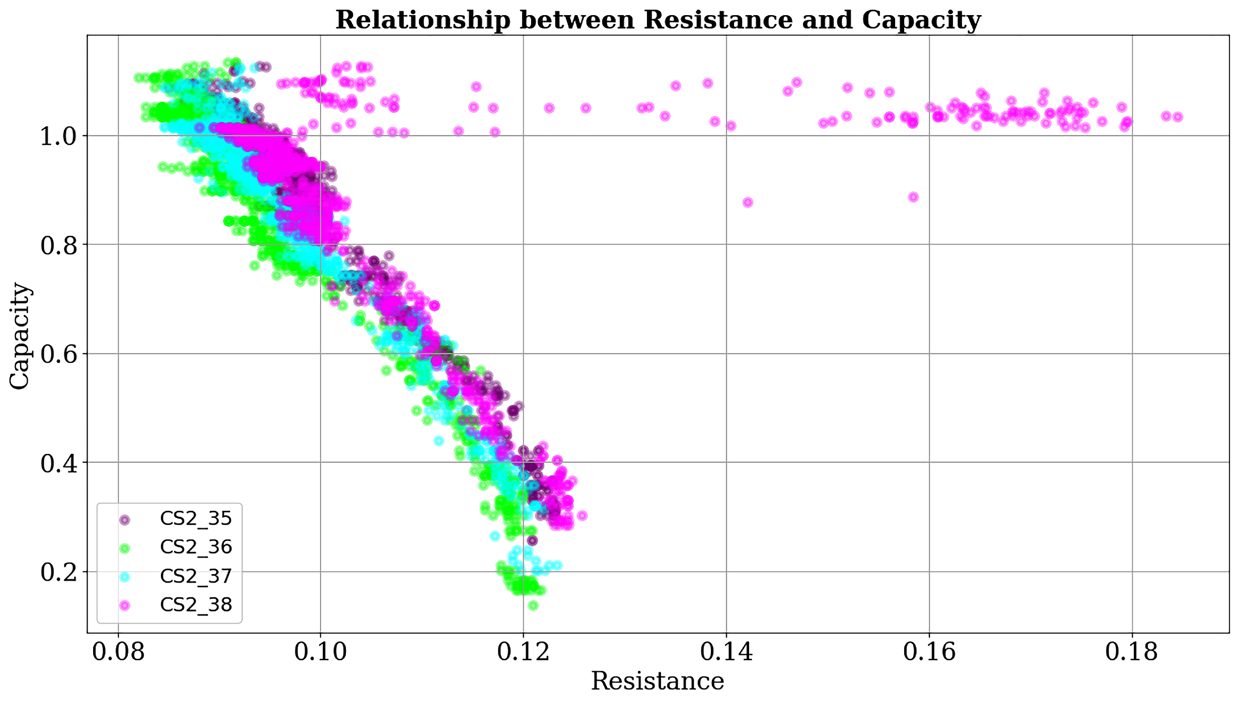
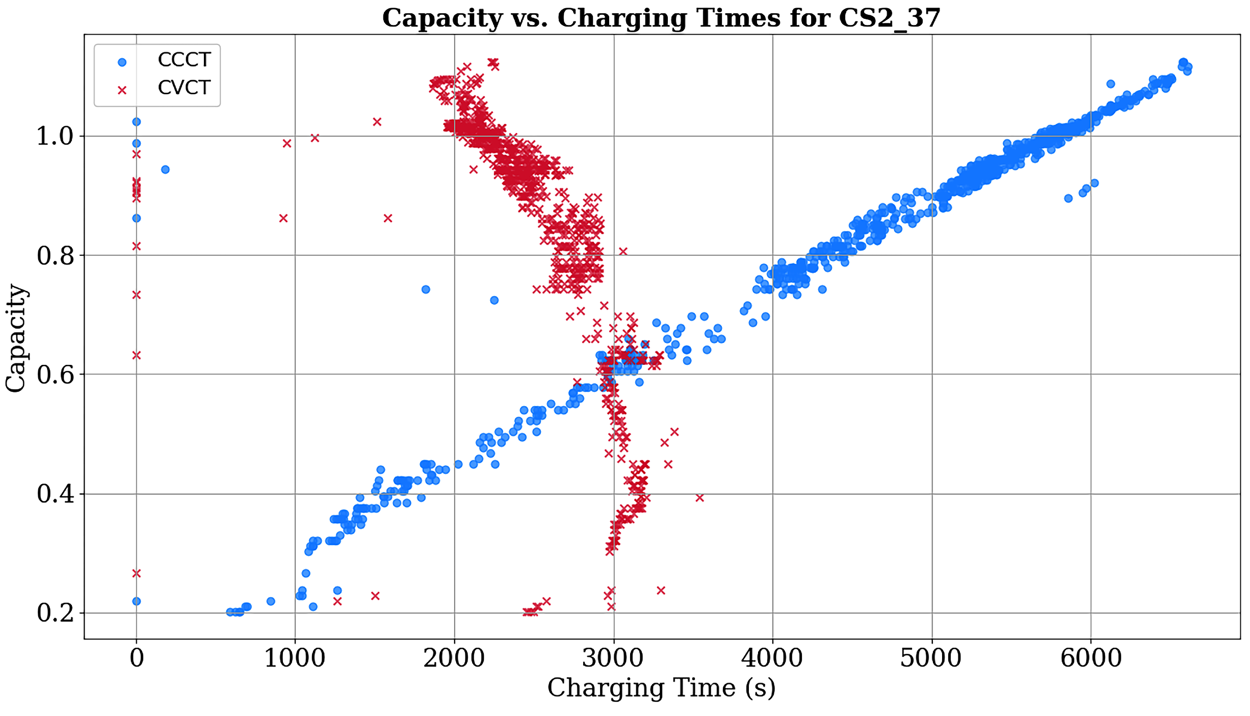
Some other parameters are in the dataset, like resistance, constant current charging time (CCCT), and constant voltage charging time (CVCT). Figure 3 shows the relationship between the battery capacity and resistance, while Figure 4 shows the relationship between the battery capacity versus CCCT and CVCT.
As the battery capacity decreased, its internal resistance value increased; the CCCT decreased with an increased number of cycles; and the CVCT fluctuated as the battery aged. Table 1 shows the technical specification of the CS2 battery.

2.2. Remaining Useful Life

The RUL can be calculated based on the SOH, considering SOH as a health index. The SOH, which is expressed as a percentage, is the ratio of the current capacity of the battery to its initial capacity when it was new:
SOH = C current C initial × 100 %
The RUL is the remaining time until the battery SOH drops below the SOH threshold, after which the battery is considered to be replaced or its health needs to be improved through maintenance:
R U L = S O H current S O H threshold rate   of   SOH   decline   per   cycle

2.3. Evaluation Metrics

  • The mean squared error (MSE) was used to check how accurately the predictive model estimated the RUL. It calculated the average square difference between the true RUL in the dataset and the model predictive RUL. The MSE formula for the battery RUL prediction is as follows:
MSE R U L = 1 N i = 1 N R U L true , i R U L pred , i 2
  • The root-mean-squared error (RMSE) is a standard method to evaluate the error of a predictive model. For a battery RUL, it calculated the square root of the average of the squared differences between the true RUL values in the dataset and the RUL values from the model prediction. For the battery RUL prediction, the RMSE equation is given as follows:
RMSE R U L = 1 N i = 1 N R U L true , i R U L pred , i 2
  • R 2 signifies how well the predictive model fit the data. For a battery RUL prediction, we calculated the proportion of variance in the actual RUL values that was predictable from the independent variables (for example, charge–discharge cycles, temperature, and voltage) used in the model. Its value is between 0 to 1. A value near to one indicates the model was working excellent. For a battery RUL prediction, the R 2 equation is as follows:
R R U L 2 = 1 i = 1 N R U L true , i R U L pred , i 2 i = 1 N R U L true , i R U L true 2

3. Research Methodology

3.1. Architecture of TransRUL

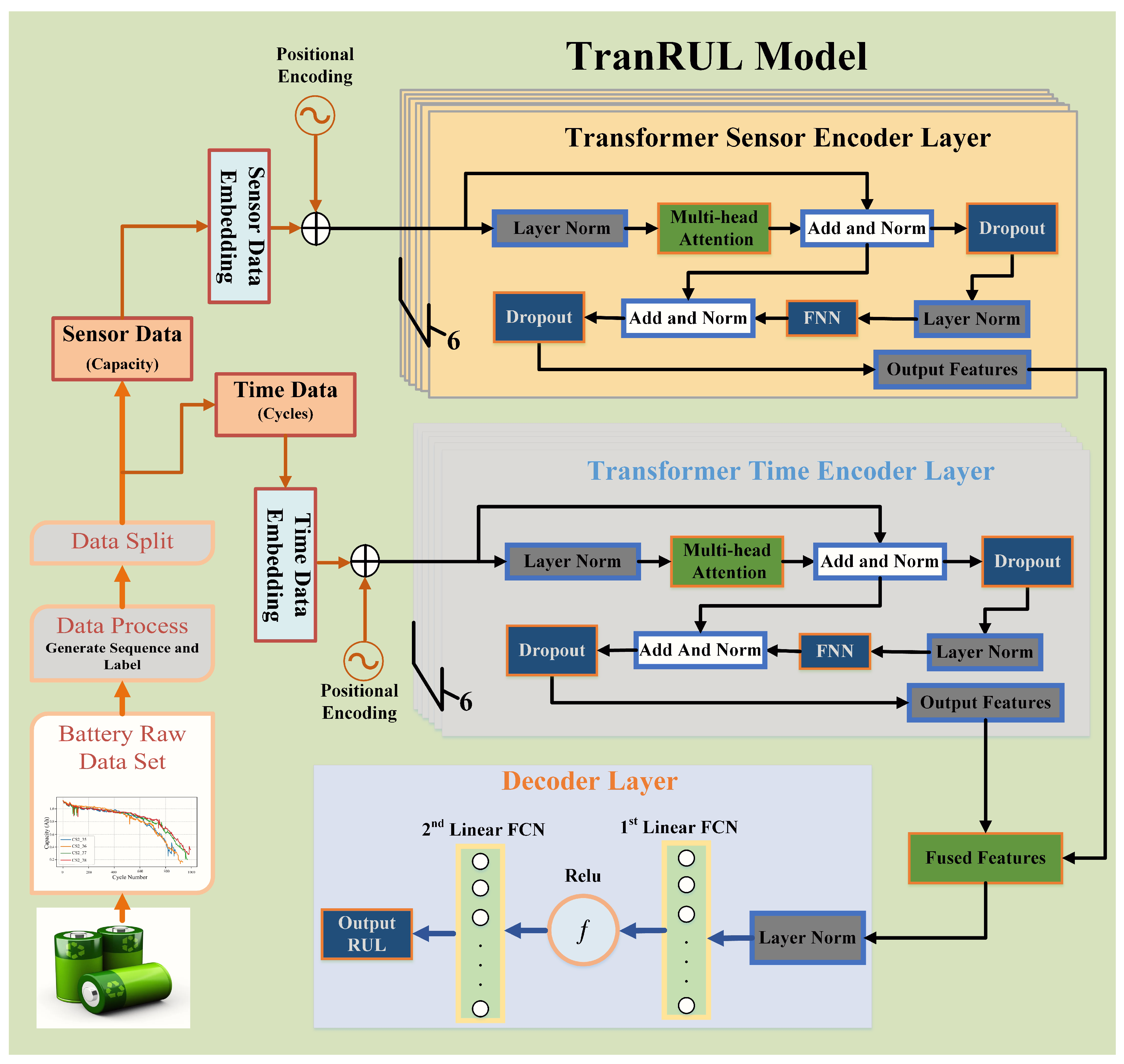
The proposed TransRUL model was specially designed for the accurate RUL prediction of LIBs and is based on a transformer with a dual encoder, positional encoding, and a multi-head attention mechanism. Figure 5 illustrates the TransRUL model architecture, which consists of many key components, each of which plays a key role in processing the input time series data to predict the LIBs’ RULs. The ability of the dual encoder architecture to capture several time series data characteristics makes it suitable for battery RUL prediction. One encoder can acquire rapid changes and transient behaviors in the battery. This is necessary to detect the changes in battery performance as soon as possible. The second encoder can track slow degradation in the battery capacity over time to provide an accurate assessment. Similarly, action and time series models are more beneficial for identifying the RUL due to recognizing short-term and long-term fading trends [28].
Positional encoding assists the model in identifying the order of the events in time series data. Every single value of the battery cycles or any time-dependent data relies on positional encoding because the model will receive it as just a set of words. This integration assists the model to differentiate between similar patterns at different times, thereby enhancing the prediction. When positional information is encoded, the same type of event at other time frames is also predicted by the model [29]. Multi-head attention allows the model to capture complicated and nuanced battery data features due to the following: (1) Parallel processing: This is because each of the attention heads may be trained to look at local features, cyclic patterns, or bursts. Parallel processing permits the model to work on several aspects of the data input at the same time, which expedites the execution. (2) Multiple perspectives: indeed, multi-head attention allows for the analysis of different data views and features altogether, which is critical for explicating the batteries’ data. (3) Capturing dependencies: This enhances the model’s ability and performance in identifying the complex inter-dependencies and relationships within the time series data. This action allows for considering different parts of the sequence at the same time, which contributes to the proper analysis of dependencies at different local and global levels [30].
These novel approaches enable the TransRUL model to handle the battery deterioration processes in order to predict the RUL with a higher accuracy. Indeed, the components of the TransRUL model, such as the dual encoder, positional encoding, and multi-head attention of the transformer, make this model highly accurate and effective for the RUL real-time estimation. The TransRUL model predicts the RULs of LIBs by capturing complex temporal dependencies and relationships within the capacity degradation data.

3.1.1. Embedding Layer

The embedding layer in the TransRUL model takes data from a sliding window as a sequence of an input batch of the shape (sequence_length, batch_size, input_dim) and converts it into a higher-dimensional space as a sequence of (sequence_length, batch_size, model_dim). This transformation of data allows the transformer encoder to process it effectively. For the battery data, this layer maps each input feature into an embedding vector of a specific dimension:
Embedding ( x ) = x × W e
where x is the input sequence, and W e is the embedding weight matrix:
X R batch   size   ×   sequence   length   ×   input   dim
W e R input   dim   ×   model   dim

3.1.2. Positional Encoding

The proposed TransRUL model does not contain structure based on a CNN or LSTM. We needed to inject some relative position tokens into the sequence so that the model can make full use of the positional information of the sequence. Positional encoding is an important component of our model that helps to understand the order of elements in the input sequence. There are currently many types of positional encoding methods available. We used a sinusoidal-based positional encoding method. Positional encoding involves vectors that are added to the input embedding. They encode the position of each entry in the sequence and ensure that the model receives information about the position of each element in the sequence. The positional encoding vectors are defined as follows:
PE ( p o s , 2 i ) = sin p o s 10,000 2 i / d m o d e l
PE ( p o s , 2 i + 1 ) = cos p o s 10,000 2 i / d m o d e l
where p o s is the position, i is the dimension, and d m o d e l is the dimension of the embedding.

3.1.3. Self-Attention Mechanism

The TransRUL model utilizes the self-attention mechanism to effectively capture the dependencies between distinct parts of the battery capacity dataset. Through the linear projection of the embedding layer, a query ( Q ), key ( K ), and value ( V ) are generated to calculate the attention score:
Q = X W Q
K = X W K
V = X W V
where W Q , W K , and W V are weight matrices, and X is a sequence of input data. The attention scorers a t are obtained by performing the dot product of the query and key matrices:
a t = Q K
Furthermore, the attention scores are scaled through the square root of the length of the key vectors ( d k ). This scaling function helps the model to stabilize during the training process:
Scaled _ a t = Q K d k
Attention weights are obtained by multiplying the scaled attention scores by the softmax function. Furthermore, these attention weights are used to produce the final output of the attention mechanism by computing the weighted sum of the value vectors:
Attention _ weights = softmax Q K d k
Output = Attention _ weights × V

3.1.4. Multi-Head Attention

The self attention model with contextual embedding can only capture a single perspective in the dataset. If there are multiple perspectives in the dataset, it cannot work properly [31]. In the TransRUL model, we used a multi-head attention mechanism (eight heads) to capture various parts of the LIBs dataset. Each attention head operates independently and focuses on several aspects of the input data sequence. By using multiple heads, the TransRUL processes various parts of the input sequence in parallel, which allows the model to work faster for RUL prediction. Each attention head works similarly, as the self-attention-generating query ( Q i ), key ( K i ), and value ( V i ) matrices use the learned linear transformations:
Q i = X W Q i
K i = X W K i
V i = X W V i
where W Q i , W K i , and W V i are the weight matrices for the i-th head.
a t _ scores i = Q i K i
Scaled _ attention _ scores i = Q i K i d k
Attention _ weights i = softmax Q i K i d k
Output i = Attention _ weights i × V i
The outputs of all the attention heads are fused to a single matrix:
Multi - Head _ Output = Concat ( Output 1 , Output 2 , , Output 8 )
Final _ Output = Multi - Head _ Output W O
Here, W O is a learned weight matrix of shape ( 8 × d k , d model ) .

3.1.5. Transformer Encoder Layer

The transformer encoder layer in our TransRUL model processes the input sequence X through six stages. Each stage is designed to capture dependencies, transform representations, and ensure stability in learning for accurate RUL prediction. The following are the components of the transformer encoder layer in our model:
  • Multi-head attention: this allows the model to simultaneously focus on various parts of the input battery data sequence.
  • Add and norm: this helps the model to remain stable and efficient during the training process by adding the input X 1 to the output of the multi-head attention mechanism and apply the normalization layer to make a combined output:
    X 1 = Final _ Output + X
    X 1 = Layer - Norm ( X 1 )
  • Position-wise feed-forward network (FFNN): This undertakes a two-step data transformation that helps our model learn more complex patterns of battery data. First, each position in the input sequence X 1 is transformed through a linear function. After this, rectified linear unit (ReLU) activation is applied to reduce the negative values.
    FFNN ( X 1 ) = max ( 0 , X 1 W 1 + b 1 )
    The output of the first step passes through another linear function in the second step to produce the final output:
    FFNN ( X 1 ) = max ( 0 , X 1 W 1 + b 1 ) W 2 + b 2
    where W is the weight and b is the bias.
  • Add and norm: This adds the input of the FFNN back to its output through residual connections and normalizes the results. This helps our model to be stable and efficient.
    X 2 = FFNN ( X 1 ) + X 1
    X 2 = Layer - Norm ( X 2 )

3.2. Working and Implementation of Proposed Method

The proposed TransRUL model accurately predicts the RULs of LIBs by taking advantage of the transformer’s self-attention mechanism to better capture the complex temporal dependencies in the battery capacity data. This model uses a dual encoder with six layers in each, one decoder, and the CALE capacity dataset of four different cells: C S _ 35 , C S _ 36 , C S _ 37 , and C S _ 38 .
Table 2 shows the arrangement of the four data groups that use these cells for the TransRUL model training and testing using LOOC validation. The working flow of the proposed model is as follows:
  • Data processing: Data processing consisted of sequence generation, labeling, and data splitting for the dual-encoder layers. We used a sliding window with size ( W = 4 ) to generate the sequences and labels. Four consecutive points in the dataset comprised a sequence and the next point in the series within the dataset was the target label:
    ( x t W : t , y t ) t = W T
    where x t W : t is the sequence and y t is the target label, which we used to calculate the loss function of the model. The sliding window over the sequence created overlapping windows that split the sequence data into sensor data corresponding to capacity values and time data corresponding to cycles within the window. The sliding window over the sequence created overlapping windows that split the sequence data into sensor data corresponding to capacity values and time data corresponding to cycles within the window.
  • Embedding and positional encoding: The embedding layers convert the sensor and time data into higher dimensional space suitable for the transformer model. The input sensor and time data size are of a tensor shape: [batch_size, window_size, 1], and they are converted to a high-dimensional tensor shape: [batch_size, window_size, 128] that passes the embedding layer:
    E sensor , time = W e x sensor , time + b e
    To retain the order sequence of the data, we added positional encoding PE at the output of sensor and time data embedding:
    Z sensor = E sensor + PE
    Z time = E time + PE
  • Sensor and time data encoder: The sensor and time data encoder have the same architecture and are configured in parallel for corresponding data processing. Each of them is composed of six layers and the following are the components of the encoder layer:
    • Layer normalization: The normalization layer in our model plays an important role in stabilizing the input data and accelerating the model-training process by maintaining the consistent activation of the mean and variance across different samples of input data:
      Z norm = Layer - Norm ( Z sensor )
    • Multi-head self-attention: In the proposed TransRUL model, the multi-head attention mechanism makes it more powerful by capturing complex relationships in the data. It improves the model’s ability to learn contextual information by focusing on different parts of the input sequence simultaneously. The details of operation are already explained in the previous section.
    • Add and norm: The add and norm operation is important for our model to improve the learning ability. It combines the layer normalization through residual connection. The residual connections are utilized to remove the vanishing gradient problems and allow gradients to flow more easily through the network. The output of the self-attention mechanism is added to the input through a residual connection and normalized:
      Z l = Layer - Norm Z sensor + Dropout ( Self - Attention ( Q l , K l , V l ) )
    • Feed-forward neural network (FFNN): The normalized output passes through an FNN. In our model, a position-wise fully connected FNN is utilized that consists of two linear transformation layers with a nonlinear ReLU activation function applied between them and it enhances the representational capacity of TransRUL model.
      FFNNN ( Z l ) = ReLU ( W 1 Z l + b 1 ) W 2 + b 2
    • Add and norm: The add and norm is used here again to combine the output of the previous normalization and the FNN through the residual connection pass through the dropout. The dropout prevents our model from over-fitting.
      Z l = Layer - Norm Z l + Dropout ( FFNN ( Z l ) )
  • Feature fusion: In the TransRUL model, the mean pooling method is used to fuse the features of the sensor and time encoders. The sensor and time data, after passing through the transformer encoder layers, have a sequence of output vectors. Therefore, to condense them into a single vector, we used the mean pooling method:
    Z sensor   mean = 1 L i = 1 L Z sensor [ i ]
    Z time   mean = 1 L i = 1 L Z time [ i ]
    where L is the sequence length, while Z sensor   mean and Z time   mean are single vectors that summarize the information. The mean-pooled values of the sensor and time features are concatenated to form the fused features:
    F = Concat ( Z sensor   mean , Z time   mean )
  • Decoder layer: The decoder in our model is used to produce output sequences and it consists of layer normalization and fully two connected layers with ReLU activation. The following are its components:
  • Layer normalization: The layer normalization in the decoder is applied to the concatenated features before being fed to fully connected layers. It helps our TransRUL model to stabilize the training process.
    F = LayerNorm ( F )
  • First linear layer: the first fully connected layer in the TransRUL decoder takes the normalized feature vector from the layer normalization and applies a linear transformation using a weight matrix W 3 and bias vector b 3 :
    F 1 = ReLU ( W 3 F norm + b 3 )
    • ReLU activation: This activation function is also important for the model because it introduces nonlinearity and allows the model to learn a more complex pattern of battery data. In our model, it is used with the first fully connected layer.
    • Second linear layer: in this layer, we again applied a linear transformation to vector F 1 through the weight matrix W 4 and bias vector b 4 :
      Y pred = W 4 F 1 + b 4
      RUL = Y pred
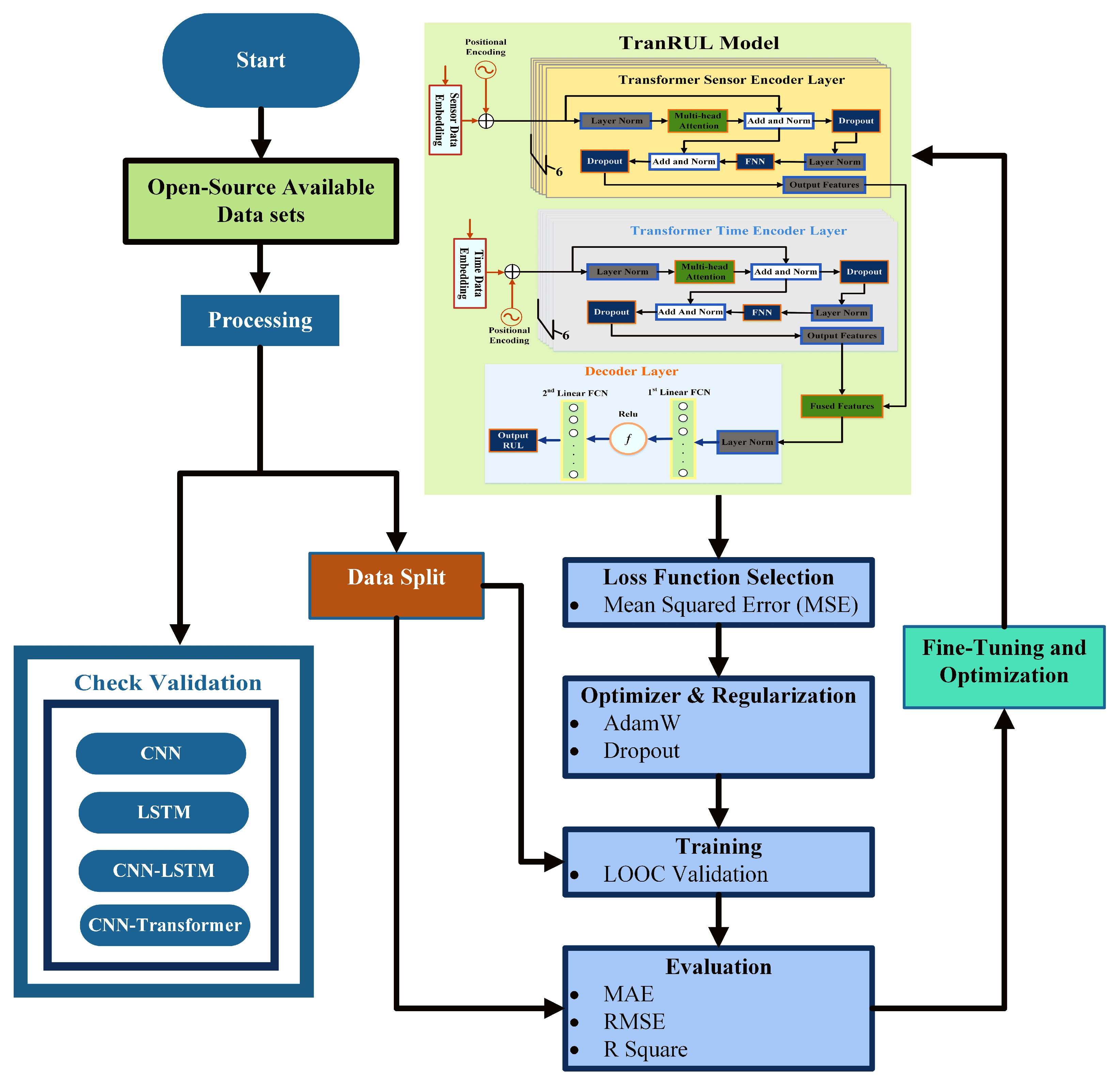
  • Model training and evaluation: To ensure the accurate prediction of the RUL, we trained and tested our TransRUL model through LOOC validation using four different groups of datasets. Figure 6 illustrates the implementation process of the TransRUL model. The training was executed for a defined number of epochs, which involved the iteration of 16 dataset batches, the calculation of the loss using the loss function MSE (mean squared error), and updating the mode parameters after comparing the predictions with the target labels. In our model, the AdamW optimizer technique was used, which made the training process more efficient by shuffling and batching the data. Table 3 shows the technical and training parameters of the proposed TransRUL model. The model was evaluated though performance metrics, including MAE, RMSE, and R 2 , which were calculated to check the accuracy. We also compared our model with some state-of-the-art methods and the latest existing research.

4. Discussion of Results

The accurate prediction of a battery RUL is critical for optimizing battery management strategies and maximizing its lifespan. This section evaluates the performance of different models for battery RUL prediction. The results highlight that the proposed TransRUL model achieved a superior prediction accuracy. The prediction results of each dataset group are described in the following sections.

4.1. Dataset Group-I

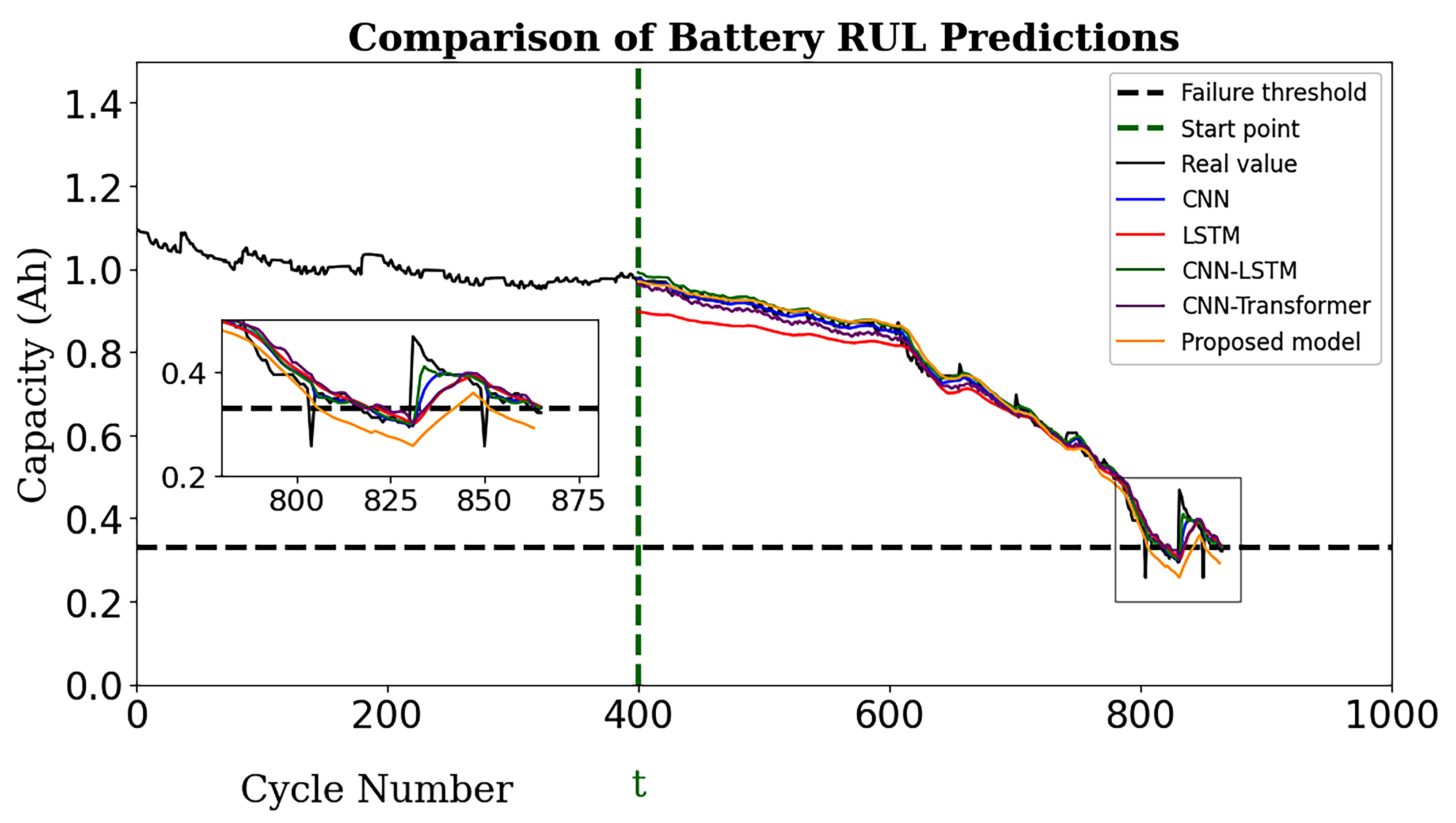
Figure 7 illustrates the comparative analysis of various models for the RUL prediction using the dataset of group-I. The x-axis denotes the cycle number, and the y-axis represents the battery capacity in ampere-hours (Ah). This capacity was used for predicting the SOH, and then the predicted SOH was used to calculate the RUL based on the threshold, which was 70 percent of the initial capacity. The five DL models—CNN, LSTM, CNN-LSTM, CNN-Transformer, and the proposed TransRUL—were compared with the actual RUL value. The observation started at 400 cycles. Various curves depict the RUL predicted by each model, and the black line represents the actual RUL value found when the SOH crossed the threshold line. For a better understanding, a zoomed section is provided that focuses on different cycles for each dataset. For dataset-I, the cycle numbers ranged from 780 to 880. The prediction results were compared after using all the methods, with the actual RUL starting from the 400th cycle and the prediction error calculated, as shown in Table 4. It can be seen from the figure and the table that the TransRUL model achieved good prediction results, with only two cycles of error, while the CNN-Transformer method had the second-lowest error, with 14 cycles.

4.2. Dataset Group-II

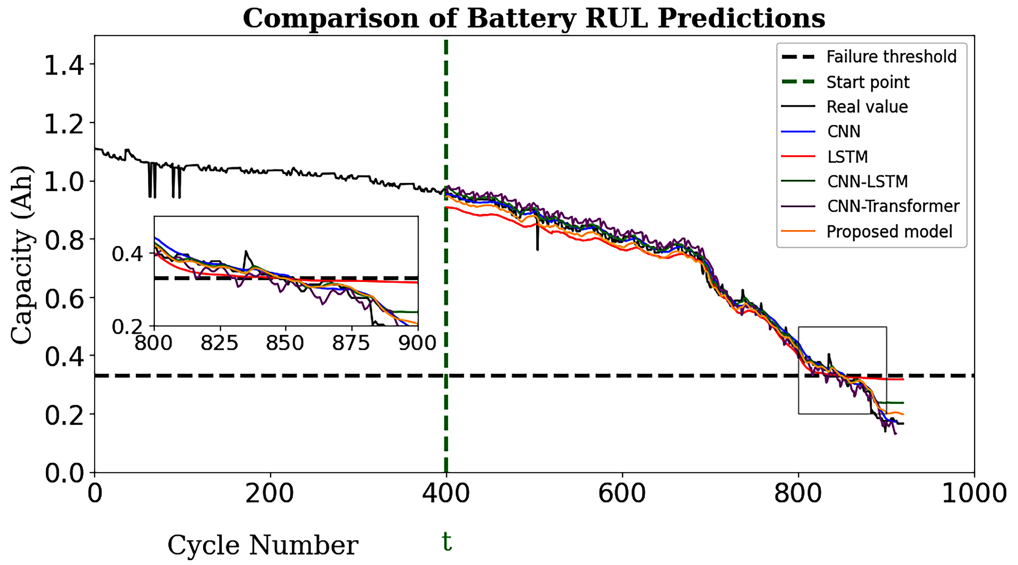
Accurate RUL predictions of LIBs are important for the effective management of energy storage systems. Figure 8 investigates the various deep learning models for RUL prediction using dataset-II. The RUL prediction accuracy of each model was evaluated by comparing it with the actual RUL values. The performance of these models was evaluated using many key metrics, and Table 5 shows the comparison. The CNN model showed a good performance, with an MAE of 0.0210, RMSE of 0.0245, and R 2 value of 0.9910. For the RUL prediction, it had an error of only 2 cycles. The LSTM has 4 cycles of error for the prediction. The CNN-Transformer model appeared to over-fit on this data group pattern, with the highest error of 34 cycles across all the models. However, the proposed TransRUL model outperformed all the other models, where it achieved the lowest MAE of 0.0074, the lowest RMSE of 0.0129, and only a 1-cycle error. The results show that the proposed model had superior precision and reliability in predicting the battery RUL.

4.3. Dataset Group-III

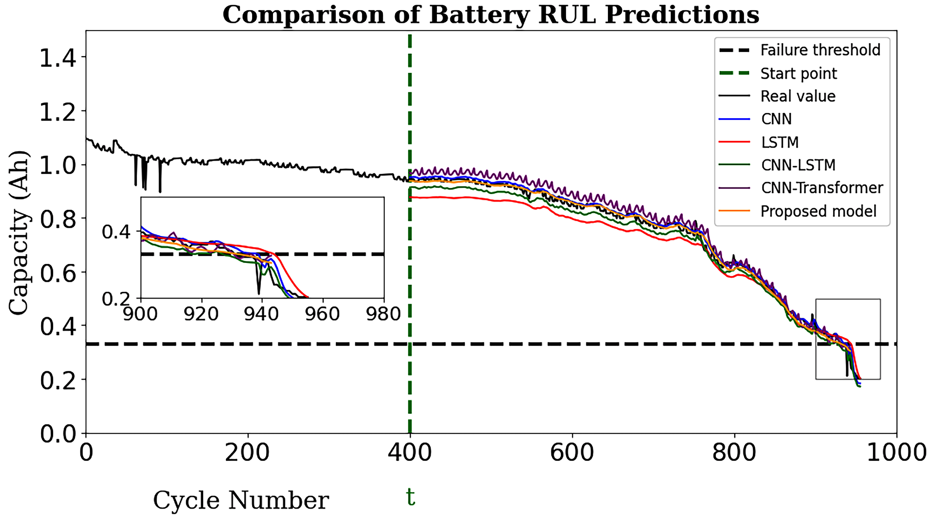
Figure 9 depicts a comprehensive evaluation of the five different DL-base models used for predicting the RUL of LIBs using dataset group-III. All the models crossed the threshold line within a cycle range of 900 to 980, and the zoomed section presents a detailed view. The observations started at 400 cycles, and the actual RUL was determined as 532 cycles. Table 6 presents key performance metrics for all the models, namely, CNN, LSTM, CNN-LSTM, CNN-Transformer, and the proposed model. It can be observed from the Figure 9 and Table 6 that the proposed TransRUL model demonstrated superior performance, with the lowest MAE (0.0069) and RMSE (0.0110), and zero error for the RUL prediction. This indicates that the proposed TransRUL model maintained close alignment with the actual data and outperformed in terms of accuracy and reliability. The CNN-Transformer model demonstrated a reasonably good prediction result, with an error of only 1 cycle. The LSTM model showed higher errors compared with CNN, with an MAE of 0.0642, an RMSE of 0.0721, and a prediction error of 12 cycles for the RUL. The CNN-LSTM shows a larger prediction error of 34 cycles. This shows that the CNN-LSTM model struggled to accurately capture the patterns present in the dataset. The results prove that the proposed TransRUL model had superior performance and provided a robust solution for battery RUL prediction.

4.4. Dataset Group-IV

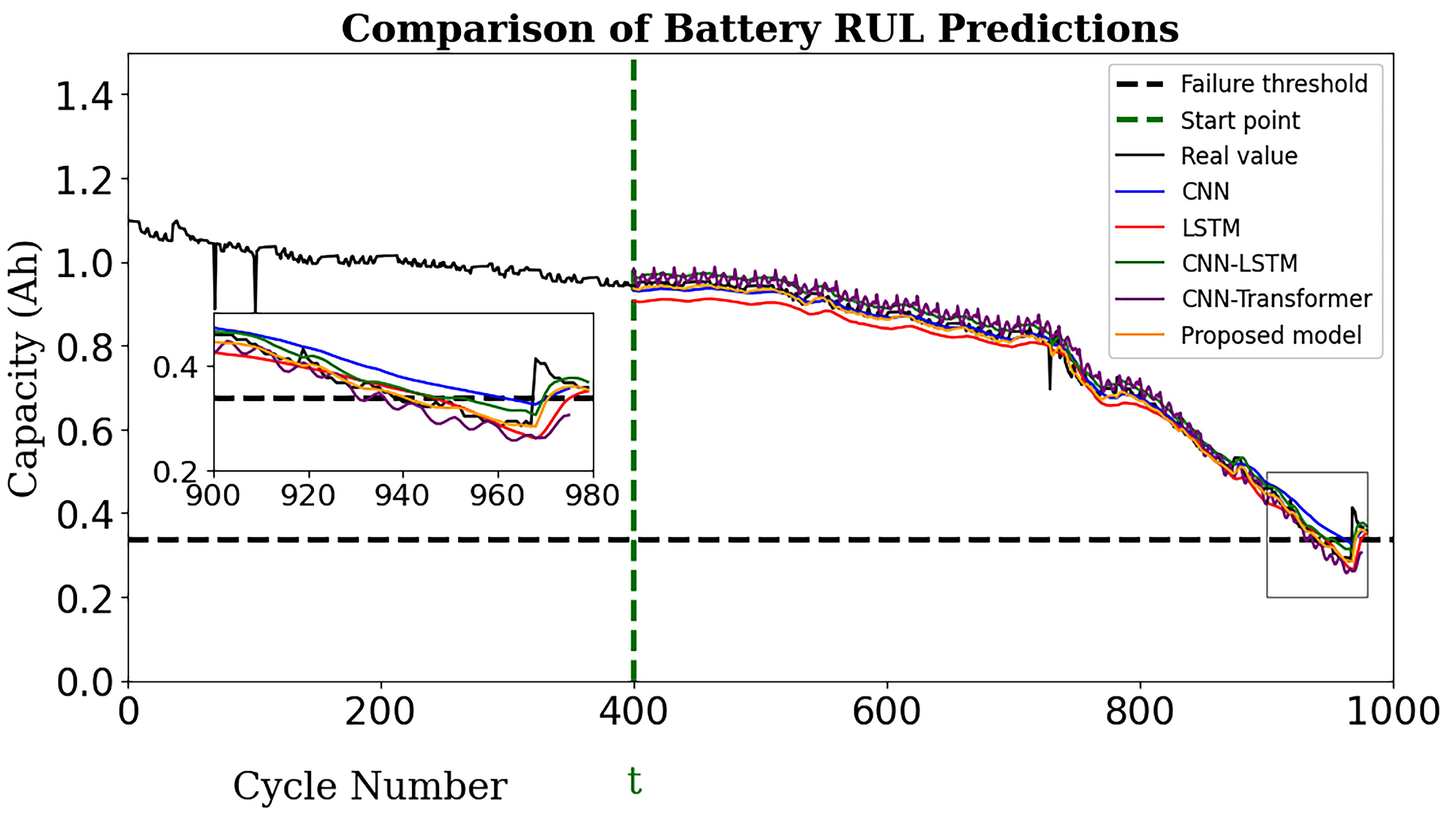
Accurate RUL predictions of LIBs is important to optimize maintenance schedules and ensure the safety and reliability of battery base systems. Figure 10 illustrates the performance comparison of various models in predicting the LIB RUL for dataset-IV, and Table 7 summarizes the performance metrics for each model. The CNN model shows fairly good results with an MAE, RMSE, and R 2 of 0.0102, 0.0153, and 0.9943, respectively, and a predicted RUL error of 7 cycles. The LSTM model had higher errors compared with the CNN model, with an MAE, RMSE, and R 2 of 0.0377, 0.0434, and 0.9545, respectively, and an improved RUL prediction, with an error of 7 cycles. The CNN-LSTM model had significant improvement in the prediction accuracy compared with dataset-I. The CNN-Transformer model also increased its performance on this dataset and had an error of 9 cycles.
The proposed model achieved a good prediction performance compared with all the others, with the lowest values for MAE, RMSE, and R 2 of 0.0075, 0.0129, and 0.9959, respectively, with an RUL error of 1 cycle. The RUL prediction results show that the TransRUL model demonstrated superior accuracy and reliability.

4.5. Comparative Analysis

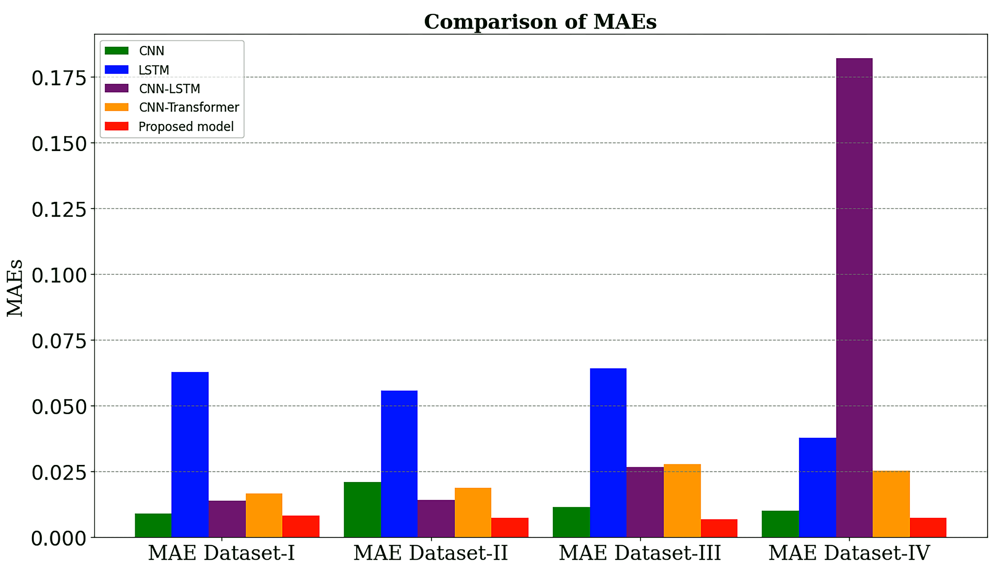
This section compares the performance of the RUL predictions of all the models discussed. The predictive accuracy of these models were compared across four groups of battery datasets using the MAE, RMSE, R 2 , and RUL prediction error as the evaluation metrics. Figure 11 and Figure 12 show the comparison of the MAE and RMSE for each model across all the datasets, and the evaluation metrics clarify the predictive accuracy of each model. In the dataset-I group, the LSTM model showed the highest MAE value of 0.0627, while the CNN, CNN-LSTM, and CNN-Transformer models showed intermediate performances. The proposed TransRUL model had the lowest MAE value of 0.0081, which suggests it had a high prediction accuracy. In dataset-II and dataset-III, the LSTM model continuously achieved the highest MAE, while the CNN-LSTM and CNN-Transformer models attained lower MAEs compared with LSTM and CNN. The proposed model maintained low MAE values using dataset-II and dataset-III, which demonstrated the consistent performance of the proposed model. In dataset-IV, the CNN-LSTM model exhibited a high MAE of 0.182, whereas CNN, LSTM, and CNN-Transformer showed moderate performances. The proposed TransRUL model showed a relatively low MAE of 0.0075 and consistently demonstrated the lowest MAE across all dataset groups. This shows that the proposed model had significantly better prediction performance compared with the other discussed models.
The LSTM model showed the highest RMSE values of 0.0733 and 0.0657 under datasets-I and -II, respectively. The CNN-LSTM, CNN, and CNN-Transformer models attained an intermediate performance. For dataset-III, the CNN-LSTM and CNN-Transformer models achieved lower RMSE values compared with LSTM and CNN. For dataset-IV, CNN-Transformer and CNN-LSTM models attained lower RMSE value as compared with LSTM. TransRUL consistently demonstrated the lowest RMSE values across all the dataset groups and provided an improved RUL prediction accuracy.
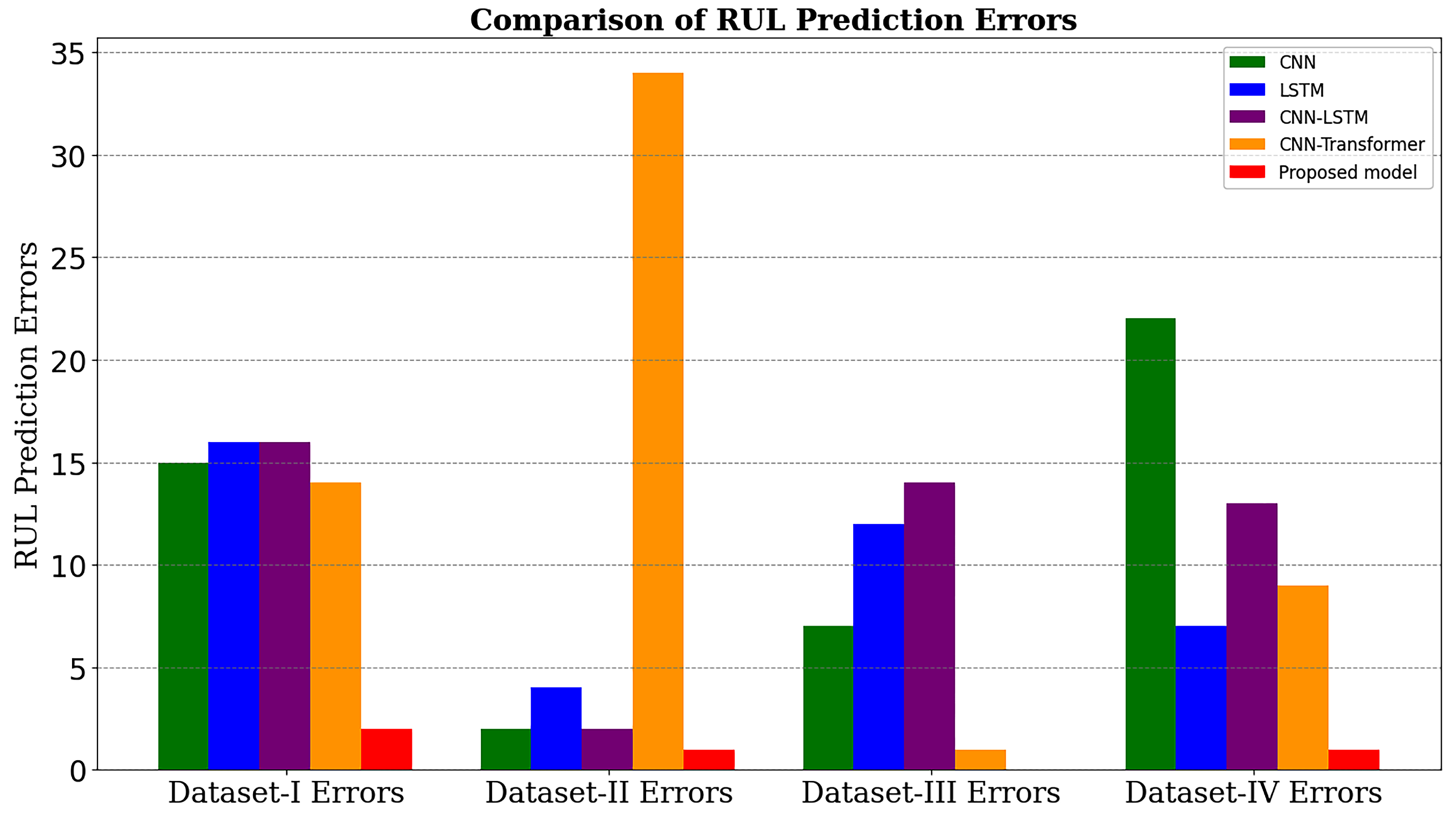
Figure 13 illustrates the RUL prediction error of different models using all the dataset groups. For dataset-I, the LSTM and CNN-LSTM models show a relatively high prediction error of 16 as compared with CNN and CNN-Transformer, while the TransRUL model had an error of two cycles. For dataset-II, the CNN-Transformer model had the worst performance, with an error of 34 cycles, while the CNN-LSTM, CNN, and LSTM models had lower RUL prediction errors as compared with CNN-Transformer. The TransRUL model achieved excellent accuracy, with an error of only one cycle. All models had the same results for dataset-III, except the TransRUL model, which had no prediction error. In the last dataset group, CNN had a higher error value of 22 and the proposed model had an error of only one cycle. The comparison results show that the TransRUL model demonstrated the lowest RUL prediction errors across all dataset groups, which proved the effectiveness of the proposed model in terms of the prediction accuracy.

4.6. Comparison with Recent Research

This section presents a comparative analysis of the proposed TransRUL model’s RUL prediction performance against some established and recent techniques through evaluating metrics for all the datasets. Table 8 and Table 9 show the comparative analysis of the proposed model with recent research.
The TransRUL model constantly proved to have a better prediction performance as compared with DL-based complete ensemble empirical mode decomposition with an adaptive noise-temporal convolutional net (CEEMDAN-TCN) [32]. It exhibited lower MAE and RMSE values and a higher R 2 , which indicates its superior accuracy in RUL prediction. A comparative evaluation of the TransRUL model against the improved sparrow search algorithm (IHSSA) in combination with the LSTM-TCN model [33] showed that the proposed model had superior performance. It can be seen from Table 8 that the proposed model had the lowest MAE and RMSE values and highest R 2 value among all the models.
The CNN-BILSTM with attention model [34] had the lowest MAE value of 0.00890 among the other models but it was still greater than the proposed model. The CNN-Transformer and particle swarm optimization with extreme learning machine (PSO-ELM)-based models had higher error values across the datasets, showing their limitation for accurate RUL prediction. The hybrid prognostic algorithm (HyA-model) [37] had good R 2 values for only the last two datasets. The proposed TransRUL model demonstrated an outstanding performance, where it consistently showed the lowest MAE and RMSE values and higher R 2 values. The values of R 2 near 1 indicate that the proposed model was more accurate in its predictions. The results show that the proposed model was highly reliable for LIB RUL prediction and highlights its potential as a leading method for RUL prediction.

4.7. Residual Analysis of the TransRUL Model

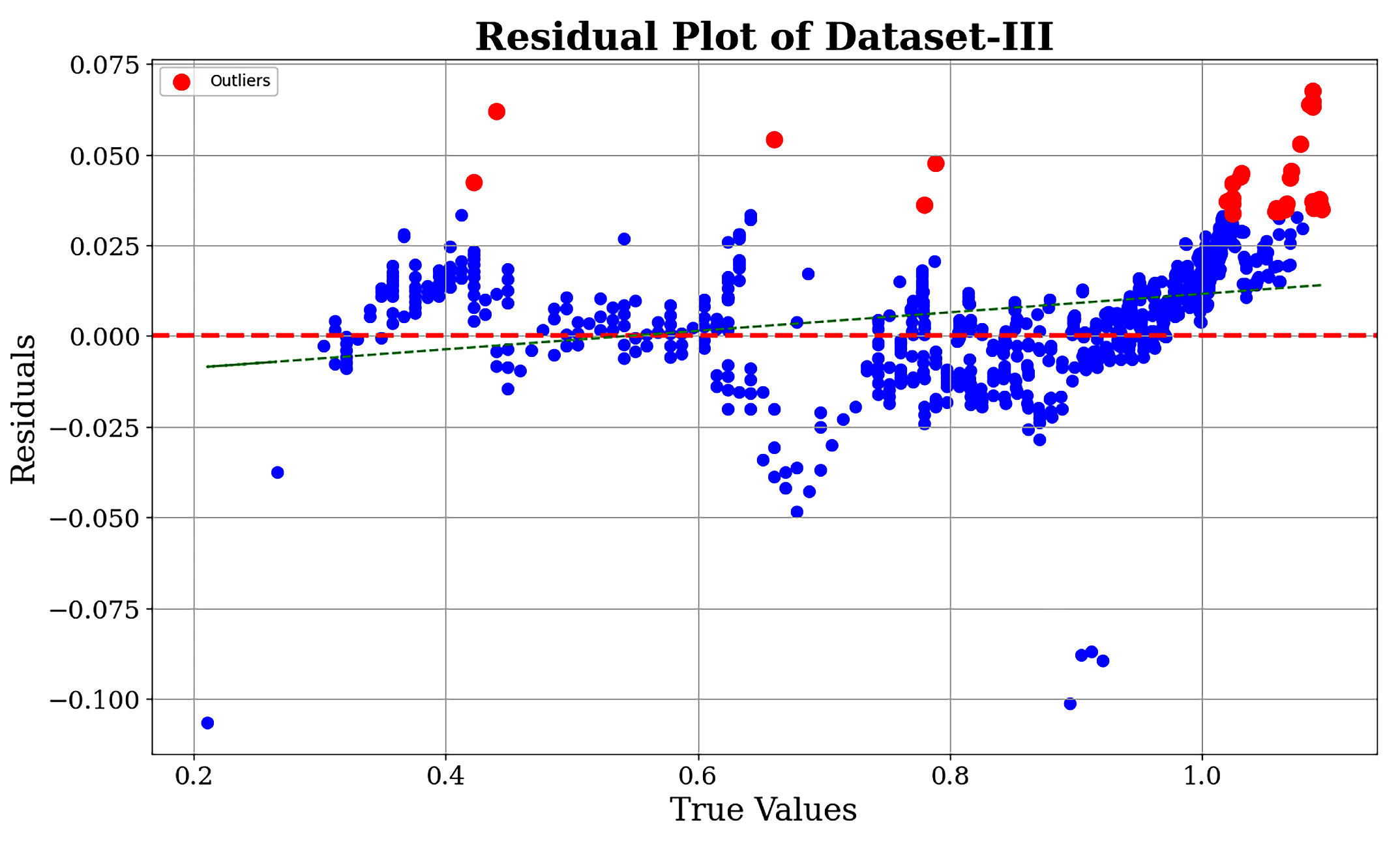
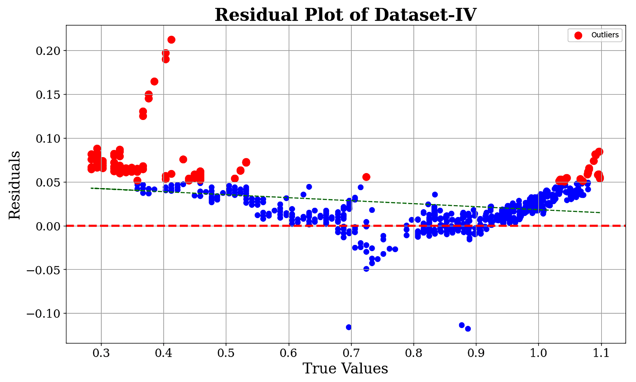
Residual analysis is widely used in predictive modeling for checking the accuracy of models, as it helps to find systematic biases or outliers and highlights their inadequacies and directions for enhancement. Figure 14 shows the residual plot of dataset-III, while Figure 15 shows the residual plot of dataset-IV.
The residuals plots of dataset-III and dataset-IV show that the majority of residual clustering appeared around the zero line, and this appeared to be true for a vast range of true values. This suggests that the model was effective and did not exhibit systematic bias for the majority of the dataset. This distribution provided a high level of confidence in the model’s accuracy in predicting a battery RUL. The analysis of the data distribution and the absence of heteroscedasticity shows evidence of the reliability of the proposed predictive model; however, some outliers were observed to be in the upper range, indicating slight underpredictions at these points. However, the overall prediction accuracy of the proposed TransRUL model was significantly good and effective.

5. Conclusions

Accurate RUL prediction is essential for the safe and reliable operation of battery-based systems. To achieve an accurate RUL prediction, this work presents a time series transformer with a dual encoder and multi-head attention based TransRUL model, where a CALCE capacity dataset of four groups was used. The TransRUL model takes raw data as the input; the sliding window technique is used to generate the sequence, labeling, and splitting into time and capacity data. Then, the positional encoding and embedding was applied to both the datasets to prepare them for the encoder input. The TransRUL model uses a dual encoder, with six sub-layers of both, and each layer of them consisted of layer normalization, multi-head attention mechanisms, and FNNs. Both the encoders use the dropout technique to prevent over-fitting. The output features from both the sensor and time encoder are fused using the mean pool method and given as the input to the model decoder. The decoder produces the final output, which is the predicted RUL that uses two FCN layers and the ReLU activation function.
To train and test the proposed model, the LOOC validation method was used in this work. To validate the performance of the TransRUL model, a rigorous experimental assessment was conducted through the CALCE dataset for four different groups. The results highlight that the TransRUL model had a higher capability to predict the RUL with a high accuracy. The proposed model consistently demonstrated low MAE and RMSE values and a higher R 2 score compared with the following benchmark DL-based methods: CNN, LSTM, CNN-LSTM, and CNN-Transformer. The proposed method’s superiority in accurately predicting the RUL compared with the recent research is also noteworthy. Despite its good performance, the proposed TransRUL model has some limitations. First, the model has complexity that can lead to a higher computational load and skill for real-time deployment. Second, the model was trained and validated only on the CS_2 battery type using four groups from the CALCE dataset, which might limit its ability on other battery types or may require additional training. Third, the reliance on large datasets for training could pose challenges in scenarios where data are scarce or expensive to obtain.
In the future, this work can be extended to a wider range of battery types and develop less computationally expensive versions for deployment with online battery management systems for proactive maintenance. This research work presents a significant advancement in the field of battery energy storage systems.
Author Contributions

U.S.: conceptualization, methodology, analysis, investigation, performing experiments on the state-of-the-art methods, model development training, validation of the results, and writing the original draft. W.L. (Weilin Li): supervision, conceptualization, and formal analysis. W.L. (Weinjie Liu): funding, supervision, review, and editing. S.R.: formal analysis and review. G.A.H.: formal analysis, review, and funding. Z.R.: Formal analysis and review. Z.A.A.: Formal analysis and review. All authors read and agreed to the published version of this manuscript.

Funding

This work was supported in part by the Natural Science Basic Research Program of Shaanxi under grant 2023-JC-QN-0599, in part by the National Natural Science Foundation of China under grant 52272403, and in part by the Fundamental Research Funds for the Central Universities. This work was also supported by The University of Dubai, United Arab Emirates.

Institutional Review Board Statement

Not applicable.

Informed Consent Statement

Not applicable.

Data Availability Statement

This work used CALCE datasets of different batteries that can be accessed at https://calce.umd.edu/battery-data, accessed on 10 March 2024.

Conflicts of Interest

The authors declare that they have no known competing financial interests or personal relationships that could have appeared to influence the work reported in this article.

References

  1. Szymczak, P.D. Lithium Drives EV, Grid Storage as Industry Scrambles To Fill Supply Deficit. J. Pet. Technol. 2022, 74, 38–43. [Google Scholar] [CrossRef]
  2. Ahmed, M.D.; Maraz, K.M. Revolutionizing energy storage: Overcoming challenges and unleashing the potential of next generation Lithium-ion battery technology. Mater. Eng. Res. 2023, 5, 265–278. [Google Scholar] [CrossRef]
  3. Qin, H.; Fan, X.; Fan, Y.; Wang, R.; Tian, F. Lithium-ion Batteries RUL Prediction Based on Temporal Pattern Attention. J. Physics: Conf. Ser. 2022, 2320, 012005. [Google Scholar] [CrossRef]
  4. Hasib, S.A.; Islam, S.; Chakrabortty, R.K.; Ryan, M.J.; Saha, D.K.; Ahamed, M.H.; Moyeen, S.I.; Das, S.K.; Ali, M.F.; Islam, M.R.; et al. A Comprehensive Review of Available Battery Datasets, RUL Prediction Approaches, and Advanced Battery Management. IEEE Access 2021, 9, 86166–86193. [Google Scholar] [CrossRef]
  5. Saha, B.; Goebel, K. Modeling Li-ion battery capacity depletion in a particle filtering framework. In Proceedings of the Annual Conference of the PHM Society, San Diego, CA, USA, 27 September–1 October 2009; Volume 1. [Google Scholar]
  6. Feng, C.; Huang, H.; Lu, G.; Zhai, J.; Zhao, Z. A Review of the Research on Remaining Useful Life Prediction Methods for Lithium-Ion Batteries. In Proceedings of the 2023 3rd International Conference on Energy, Power and Electrical Engineering (EPEE), Wuhan, China, 15–17 September 2023; pp. 565–571. [Google Scholar] [CrossRef]
  7. Saleem, U.; Li, W.; Liu, W.; Ahmad, I.; Aslam, M.M.; Lateef, H.U. Investigation of Deep Learning Based Techniques for Prognostic and Health Management of Lithium-Ion Battery. In Proceedings of the 2023 15th International Conference on Electronics, Computers and Artificial Intelligence (ECAI), Bucharest, Romania, 29–30 June 2023; pp. 1–6. [Google Scholar] [CrossRef]
  8. Saleem, U.; Liu, W.; Li, W.; Sardar, M.U.; Aslam, M.M.; Riaz, S. Enhancing PHM System of Aircraft Generator with Machine Learning-Driven Faults Classification. In Proceedings of the 2024 ASU International Conference in Emerging Technologies for Sustainability and Intelligent Systems (ICETSIS), Manama, Bahrain, 28–29 January 2024; pp. 1–5. [Google Scholar] [CrossRef]
  9. Zhang, Y.; Xiong, R.; He, H.; Pecht, M. Long Short-Term Memory Recurrent Neural Network for Remaining Useful Life Prediction of Lithium-Ion Batteries. IEEE Trans. Veh. Technol. 2018, 67, 5695–5705. [Google Scholar] [CrossRef]
  10. Ren, L.; Dong, J.X.; Wang, X.; Meng, Z.; Zhao, L.; Deen, M. A Data-Driven Auto-CNN-LSTM Prediction Model for Lithium-Ion Battery Remaining Useful Life. IEEE Trans. Ind. Inform. 2021, 17, 3478–3487. [Google Scholar] [CrossRef]
  11. Xu, X.; Wu, Q.; Li, X.; Huang, B. Dilated Convolution Neural Network for Remaining Useful Life Prediction. J. Comput. Inf. Sci. Eng. 2020, 20, 021004. [Google Scholar] [CrossRef]
  12. Abiodun, O.I.; Jantan, A.; Omolara, A.E.; Dada, K.V.; Mohamed, N.; Arshad, H. State-of-the-art in artificial neural network applications: A survey. Heliyon 2018, 4, e00938. [Google Scholar] [CrossRef] [PubMed]
  13. Cui, Z.; Ke, R.; Pu, Z.; Wang, Y. Stacked Bidirectional and Unidirectional LSTM Recurrent Neural Network for Forecasting Network-wide Traffic State with Missing Values. Transp. Res. Part C Emerg. Technol. 2020, 118, 102674. [Google Scholar] [CrossRef]
  14. Wang, X.; Li, J.; Shia, B.C.; Kao, Y.W.; Ho, C.W.; Chen, M. A Novel Prediction Process of the Remaining Useful Life of Electric Vehicle Battery Using Real-World Data. Processes 2021, 9, 2174. [Google Scholar] [CrossRef]
  15. Ardeshiri, R.R.; Ma, C. Multivariate gated recurrent unit for battery remaining useful life prediction: A deep learning approach. Int. J. Energy Res. 2021, 45, 16633–16648. [Google Scholar] [CrossRef]
  16. Wei, M.; Gu, H.; Ye, M.; Wang, Q.; Xu, X.; Wu, C. Remaining useful life prediction of lithium-ion batteries based on Monte Carlo Dropout and gated recurrent unit. Energy Rep. 2021, 7, 2862–2871. [Google Scholar] [CrossRef]
  17. Ahmad, I.; Ahmad, M.A.; Anwar, S.J. Transfer Learning and Dual Attention Network Based Nuclei Segmentation in Head and Neck Digital Cancer Histology Images. In Proceedings of the 2023 15th International Conference on Electronics, Computers and Artificial Intelligence (ECAI), Bucharest, Romania, 29–30 June 2023; pp. 1–5. [Google Scholar] [CrossRef]
  18. Liu, R.; Xie, M.; Liu, A.; Song, H. Joint Optimization Risk Factor and Energy Consumption in IoT Networks with TinyML-Enabled Internet of UAVs. IEEE Internet Things J. 2024, 11, 20983–20994. [Google Scholar] [CrossRef]
  19. Chen, M.; Yi, M.; Huang, M.; Huang, G.; Ren, Y.; Liu, A. A novel deep policy gradient action quantization for trusted collaborative computation in intelligent vehicle networks. Expert Syst. Appl. 2023, 221, 119743. [Google Scholar] [CrossRef]
  20. Li, L.; Li, Y.; Mao, R.; Li, L.; Hua, W.; Zhang, J. Remaining Useful Life Prediction for Lithium-Ion Batteries With a Hybrid Model Based on TCN-GRU-DNN and Dual Attention Mechanism. IEEE Trans. Transp. Electrif. 2023, 9, 4726–4740. [Google Scholar] [CrossRef]
  21. Zhao, J.; Han, X.; Ouyang, M.; Burke, A.F. Specialized deep neural networks for battery health prognostics: Opportunities and challenges. J. Energy Chem. 2023, 87, 416–438. [Google Scholar] [CrossRef]
  22. Singh, S.; Budarapu, P. Deep machine learning approaches for battery health monitoring. Energy 2024, 300, 131540. [Google Scholar] [CrossRef]
  23. Chen, X.; Liu, Z.; Sheng, H.; Wu, K.; Mi, J.; Li, Q. Transfer learning based remaining useful life prediction of lithium-ion battery considering capacity regeneration phenomenon. J. Energy Storage 2024, 76, 109798. [Google Scholar] [CrossRef]
  24. Han, Y.; Li, C.; Zheng, L.; Lei, G.; Li, L. Remaining Useful Life Prediction of Lithium-Ion Batteries by Using a Denoising Transformer-Based Neural Network. Energies 2023, 16, 6328. [Google Scholar] [CrossRef]
  25. Galatro, D.; da Silva, C.; Romero, D.A.; Trescases, O.; Amon, C. Challenges in data-based degradation models for lithium-ion batteries. Int. J. Energy Res. 2020, 44, 3954–3975. [Google Scholar] [CrossRef]
  26. Chen, Z.; Chen, L.; Shen, W.; Xu, K. Remaining Useful Life Prediction of Lithium-Ion Battery via a Sequence Decomposition and Deep Learning Integrated Approach. IEEE Trans. Veh. Technol. 2022, 71, 1466–1479. [Google Scholar] [CrossRef]
  27. Mo, H.; Iacca, G. Evolutionary neural architecture search on transformers for RUL prediction. Mater. Manuf. Process. 2023, 38, 1881–1898. [Google Scholar] [CrossRef]
  28. Yu, Z.; Wang, J.; Yu, L.C.; Zhang, X. Dual-encoder transformers with cross-modal alignment for multimodal aspect-based sentiment analysis. In Proceedings of the 2nd Conference of the Asia-Pacific Chapter of the Association for Computational Linguistics and the 12th International Joint Conference on Natural Language Processing, Taipei, 21–23 November 2022; Volume 1, Long Papers. pp. 414–423. [Google Scholar]
  29. Rajput, S.; Mehta, N.; Singh, A.; Keshavan, R.H.; Vu, T.; Heldt, L.; Hong, L.; Tay, Y.; Tran, V.Q.; Samost, J.; et al. Recommender Systems with Generative Retrieval. In Proceedings of the 37th Conference on Neural Information Processing Systems, New Orleans, LA, USA, 10–16 December 2023. [Google Scholar]
  30. Lin, A.; Chen, B.; Xu, J.; Zhang, Z.; Lu, G.; Zhang, D. DS-TransUNet: Dual Swin Transformer U-Net for Medical Image Segmentation. IEEE Trans. Instrum. Meas. 2022, 71, 1–15. [Google Scholar] [CrossRef]
  31. Ahmad, I.; Xia, Y.; Cui, H.; Islam, Z.U. DAN-NucNet: A dual attention based framework for nuclei segmentation in cancer histology images under wild clinical conditions. Expert Syst. Appl. 2023, 213, 118945. [Google Scholar] [CrossRef]
  32. Zhao, J.; Liu, D.; Meng, L. Remaining useful life prediction of a lithium-ion battery based on a temporal convolutional network with data extension. Int. J. Appl. Math. Comput. Sci. 2024, 34, 105–117. [Google Scholar] [CrossRef]
  33. Qiu, S.; Zhang, B.; Lv, Y.; Zhang, J.; Zhang, C. A Lithium-Ion Battery Remaining Useful Life Prediction Model Based on CEEMDAN Data Preprocessing and HSSA-LSTM-TCN. World Electr. Veh. J. 2024, 15, 177. [Google Scholar] [CrossRef]
  34. Li, C.; Han, X.; Zhang, Q.; Li, M.; Rao, Z.; Liao, W.; Liu, X.; Liu, X.; Li, G. State-of-health and remaining-useful-life estimations of lithium-ion battery based on temporal convolutional network-long short-term memory. J. Energy Storage 2023, 74, 109498. [Google Scholar] [CrossRef]
  35. Wu, Y.; Li, W.; Wang, Y.; Zhang, K. Remaining Useful Life Prediction of Lithium-Ion Batteries Using Neural Network and Bat-Based Particle Filter. IEEE Access 2019, 7, 54843–54854. [Google Scholar] [CrossRef]
  36. Wang, G.; Sun, L.; Wang, A.; Jiao, J.; Xie, J. Lithium battery remaining useful life prediction using VMD fusion with attention mechanism and TCN. J. Energy Storage 2024, 93, 112330. [Google Scholar] [CrossRef]
  37. Pugalenthi, K.; Park, H.; Hussain, S.; Raghavan, N. Hybrid Particle Filter Trained Neural Network for Prognosis of Lithium-Ion Batteries. IEEE Access 2021, 9, 135132–135143. [Google Scholar] [CrossRef]
  38. Yao, F.; He, W.; Wu, Y.; Ding, F.; Meng, D. Remaining useful life prediction of lithium-ion batteries using a hybrid model. Energy 2022, 248, 123622. [Google Scholar] [CrossRef]
  39. Ma, Y.; Li, J.; Hu, Y.; Chen, H. A Battery Prognostics and Health Management Technique Based on Knee Critical Interval and Linear Complexity Self-Attention Transformer in Electric Vehicles. IEEE Trans. Intell. Transp. Syst. 2024, 25, 10216–10230. [Google Scholar] [CrossRef]
Figure 1. Battery RUL prediction using capacity degradation pattern.
Energies 17 03976 g001
Figure 2. CALCE capacity dataset.
Energies 17 03976 g002
Figure 3. Relationship between battery capacity and resistance.
Energies 17 03976 g003
Figure 4. Relationship between battery capacity, CCCT, and CVCT.
Energies 17 03976 g004
Figure 5. Architecture of proposed TransRUL model.
Energies 17 03976 g005
Figure 6. Implementation of proposed model workflow.
Energies 17 03976 g006
Figure 7. RUL prediction results of dataset group-I.
Energies 17 03976 g007
Figure 8. RUL prediction results for dataset group-II.
Energies 17 03976 g008
Figure 9. RUL prediction results for dataset group-III.
Energies 17 03976 g009
Figure 10. RUL prediction results of dataset group-IV.
Energies 17 03976 g010
Figure 11. Prediction comparison of MAE errors for all dataset groups.
Energies 17 03976 g011
Figure 12. Prediction comparison of RMSE errors for all dataset groups.
Energies 17 03976 g012
Figure 13. Comparison of RUL prediction errors of all dataset groups.
Energies 17 03976 g013
Figure 14. Residual plot of dataset-III.
Energies 17 03976 g014
Figure 15. Residual plot of dataset-IV.
Energies 17 03976 g015
Table 1. Technical parameters of battery CS2.
Battery CellsParameterValues
CS2_35Nominal voltage4.2 V
CS2_36Energy capacity1.1 Ah
CS2_37Charging current0.55 A
CS2_38Discharging current1.1 A
Voltage range4.2 V to 2.7 V (discharge)
Physical Dimensions
Length5.4 mm
Width33.6 mm
Height50.6 mm
Table 2. Data group arrangements.
Dataset ArrangementFor Training PurposesTesting
Group ICS2_36, CS2_37, and CS2_38CS2_35
Group IICS2_35, CS2_37, and CS2_38CS2_36
Group IIICS2_35, CS2_36, and CS2_38CS2_37
Group IVCS2_35, CS2_36, and CS2_37CS2_38
Table 3. Technical and training parameters for the TransRUL model.
ParameterValue
Model architectureTransformer with dual encoder
Input dimension1
Model dimension128
Number of encoder layers6
Number of decoder layers1 (single linear transformation layer)
Number of heads8
Dropout rate0.1
Positional encodingYes
Batch size16
Learning rate0.0001
Loss functionMean squared error (MSE)
OptimizerAdamW
Training epochs1500
Validation methodLOOC (leave-one-out cross-validation)
DatasetCALCE capacity dataset, four groups
Table 4. Comparison of prediction results of dataset-I through evolution metrics.
Model NameMAERMSE R 2 Accurate RULPredicted RULError (Cycles)
CNN0.00890.01510.994740441915
LSTM0.06270.07330.874740442016
CNN-LSTM0.01380.01820.992340442016
CNN-Transformer0.01650.02250.98840441814
Proposed model0.00810.01300.99614044062
Table 5. Comparison of prediction results of dataset-II through evolution metrics.
Model NameMAERMSE R 2 Accurate RULPredicted RULError (Cycles)
CNN0.02100.02450.99104504522
LSTM0.05560.06570.93534504464
CNN-LSTM0.01410.02060.99364504482
CNN-Transformer0.01890.02710.988245041634
Proposed model0.00740.01290.99894504491
Table 6. Comparison of prediction results of dataset-III through evolution metrics.
Model NameMAERMSE R 2 Accurate RULPredicted RULError (Cycles)
CNN0.01150.01600.99405325397
LSTM0.06420.07210.878453254412
CNN-LSTM0.02660.02850.981153251814
CNN-Transformer0.02780.03110.97735325311
Proposed model0.00690.01100.99675325320
Table 7. Comparison of prediction results of dataset-IV through evolution metrics.
Model NameMAERMSE R 2 Accurate RULPredicted RULError (Cycles)
CNN0.01020.01530.994354056222
LSTM0.03770.04340.95455405477
CNN-LSTM0.18200.02430.985854055313
CNN-Transformer0.02530.03010.97815405319
Proposed model0.00750.01290.99595405411
Table 8. Comparison of prediction results with other research (datasets-I and -II).
Model NameDataset-I (CS2-35)Dataset-II (CS2-36)
MAERMSER2MAERMSER2
CEEMDAN-TCN [32]0.03930.0499-0.05360.0736-
HSSA-LSTM-TCN [33]0.01970.03370-0.01940.0257-
CNN-BILSTM with attention [34]0.008900.014900.994900.011600.021300.99320
ANN-PF [35]-0.01420.9902-0.01380.9917
VMD fusion with attention and TCN [36]0.01320.01530.99180.01130.01360.9936
HyA-model [37]------
PSO-ELM [38]------
CNN-Transformer [39]0.07160.0901-0.06310.0802-
Proposed model0.00810.01300.99610.00740.01290.9975
Table 9. Comparison of prediction results with other research (datasets-III and -IV).
Model NameDataset-III (CS2-37)Dataset-IV (CS2-38)
MAERMSER2MAERMSER2
CEEMDAN-TCN [32]0.02700.0352-0.05590.0538-
HSSA-LSTM-TCN [33]0.04250.0497----
CNN-BILSTM with attention [34]0.00800.014900.994900.015000.01780.99230
ANN-PF [35]-0.01270.9913-0.01320.9910
Wang2024 [13]0.01050.01360.99350.00870.01100.9958
HyA-model [37]--0.050--0.047
PSO-ELM [38]--0.2047-0.09338-
CNN-Transformer [39]---0.09950.1306-
Proposed model0.00690.01100.99670.00750.01290.9959
Disclaimer/Publisher’s Note: The statements, opinions and data contained in all publications are solely those of the individual author(s) and contributor(s) and not of MDPI and/or the editor(s). MDPI and/or the editor(s) disclaim responsibility for any injury to people or property resulting from any ideas, methods, instructions or products referred to in the content.