Article

Improved Model-Free Predictive Control of a Three-Phase Inverter

by
Muhammad Nauman
and
Wajiha Shireen
*
Department of Electrical and Computer Engineering, University of Houston, Houston, TX 77004, USA
*
Author to whom correspondence should be addressed.
Energies 2024, 17(15), 3761; https://doi.org/10.3390/en17153761
Submission received: 27 June 2024 / Revised: 21 July 2024 / Accepted: 26 July 2024 / Published: 30 July 2024
(This article belongs to the Special Issue Power Quality and Hosting Capacity in the Microgrids)

Abstract

:
Model predictive control (MPC) performance depends on the accuracy of the system model. Moreover, the optimization algorithm of MPC requires numerous online computations. These inherent limitations of MPC hinder its application in power electronics systems. This paper proposes a two-part solution for these challenges for a three-phase inverter with an output LC filter. The first part of the control scheme is a linear and modified model-free approach based on the auto-regressive structure (ARX) with exogenous input. The second part is the computationally efficient optimization algorithm based on the active set method to solve the optimization problem of the MFPC. The objective of the control scheme is to regulate the output voltages of the inverter in the presence of constraints. The constraints are the maximum admissible filter current and optimal duty cycle to avoid any damage to the system. To validate the performance of the proposed control scheme, simulations and hardware-in-loop (HIL) real-time investigations have been performed, comparing the results of the proposed approach with the model-based predictive control. The results showcase the computational efficiency and effectiveness of the MFPC approach, demonstrating its potential for overcoming the limitations of traditional MPC in power electronics systems.

1. Introduction

Three-phase inverter with an LC filter is the most commonly used topology for providing sinusoidal voltages with low total harmonic distortion (THD) [1]. This topology has a lot of significance for applications which require pure sinusoidal voltages at their output such as uninterruptible power supplies (UPSs), electric drives, and the integration of distributed energy resources (DERs) with the AC grid [2,3,4]. The primary control objective for this topology is to regulate the output voltages to the desired reference levels while considering system constraints such as maximum permissible filter current or limitations on the input [5].
Model predictive control (MPC) is a viable option for constrained power electronic systems due to its ability to systematically handle constraints, its simple design concepts, and its fast dynamic response [6]. Both versions of MPC, implicit [7] and explicit [8], have been proposed for power converters. Implicit MPC has been applied to three-phase inverters with LC filter [5]. To reduce the computational burden of implicit MPC, explicit MPC has been proposed for PWM inverters [6]. However, regardless of whether implicit or explicit MPC is used, as a model-based approach, the performance of MPC is dependent on the accuracy of the system model [9]. Any mismatch in the system model can significantly affect controller performance. Additionally, a major drawback of implicit MPC is the high computational requirement to determine the optimal control action [10].
Model-free predictive control (MFPC) has been proposed to eliminate the dependence of MPC on the system model [11]. MFPC consists of two parts: a model-free approach and predictive control (PC) [12]. The model-free approach estimates the future behavior of system variables, while the predictive controller uses a cost function as a criterion to determine the optimal control action. Additionally, MFPC handles constraints in the same systematic way as MPC. Due to these advantages, MFPC is increasingly being applied to power converters [13].
A finite control set model predictive control (FCS-MFPC) has been proposed for voltage source inverters with a first-order filter at the output [14]. However, due to the FCS approach, this control scheme suffers from variable switching frequencies. Furthermore, system constraints are not included in the proposed FCS-MFPC. FCS-MPC has also been proposed for grid-forming inverters with LCL filters [15]. The proposed FCS-MFPC cost function incorporated a switching penalizing term to reduce switching effort and a voltage tracking error term to better track capacitor voltages. However, the proposed approach does not include the system constraint of the maximum permissible filter current. An FCS data-driven predictive control has been proposed for the electric drives [16]. The proposed approach regulates the stator current in the presence of constraints on the stator current. However, there are no constraints that can deal with the variable switching frequency of the FCS-MPC.
To solve the problems mentioned above, this paper proposed a model-free predictive control that is computationally efficient and does not require the physical model of the system. The contributions of this paper are summarized as follows:
  • The proposed approach uses a continuous control set-based MFPC to control a three-phase inverter with an LC filter in the presence of the system constraints. The CCS approach eliminates the problem of variable switching frequency and provides sinusoidal voltages of low THD.
  • The model-free approach uses an auto-regressive structure with exogenous input (ARX) to estimate the system dynamics. ARX is a linear parametric model that reduces the complexity of the proposed approach. Moreover, a well-established method of recursive least squares (RLS) is available to be used to estimate ARX parameters.
  • The system constraints of the maximum permissible filter current and duty cycle constraints are part of the control.
  • A computationally efficient optimization algorithm based on an active set method (ASM). The computations of ASM depend on the number of constraints. The system constraints are reduced by combining the constraints of the maximum permissible filter current and duty cycle due to their dependence on each other.
  • A detailed stability analysis of the proposed MFPC has been presented using the Lyapunov theory.
The organization of this paper is as follows. Section 2 discusses the mathematical modeling of the system. Section 4 explains MFPC formulation for the three-phase inverter with LC filter. Section 7 discusses the simulation results of the proposed MFPC approach and its comparison with MPC. Finally, Section 10 concludes the paper.

2. System Modeling

A two-level three-phase inverter with LC filter is shown in Figure 1. Each leg of the inverter has two switches that will operate in complementary mode. i f a , i f b and i f c are the filter currents with a filter inductance of L in each phase. v a n , v b n and v c n are the output voltages of the inverter with a filter capacitance of C in each phase. A balanced three-phase and unknown load is connected at the output of the inverter and it draws current i o a , i o b and i o c . The input of the inverter is the constant DC voltage v d c .

2.1. Continuous-Time State-Space Model

The states of the switches S 1 S 6 are represented by the switching signals S a , S b and S c . These switching signals are defined as
S a = 1 if S 1 = 1 and S 2 = 0 0 if S 1 = 0 and S 2 = 1
S b = 1 if S 3 = 1 and S 4 = 0 0 if S 3 = 0 and S 4 = 1
S c = 1 if S 5 = 1 and S 6 = 0 0 if S 5 = 0 and S 6 = 1
The continuous state-space form of the three-phase inverter with LC filter is defined as:
d x d t = A x + B u + B d i o
with,
A = 0 0 0 1 L 0 0 0 0 0 0 1 L 0 0 0 0 0 0 1 L 1 C 0 0 0 0 0 0 1 C 0 0 0 0 0 0 1 C 0 0 0 ,   B = 1 L 0 0 0 1 L 0 0 0 1 L 0 0 0 0 0 0 0 0 0 ,   B d = 0 0 0 0 0 0 0 0 0 1 C 0 0 0 1 C 0 0 0 1 C .
i o = i o a i o b i o c ,   x = i f a i f b i f c v a n v b n v c n ,   u = S a V d c ( S a + S b + S c 3 ) V d c S b V d c ( S a + S b + S c 3 ) V d c S c V d c ( S a + S b + S c 3 ) V d c 0 0 0 .
The system in (4) is a non-linear system because of the switching signals S a , S b , and S c .

2.2. Discrete-Time State-Space Model

To linearize the system described in (4), we use the state-space averaging [3] technique. Moreover, to obtain a discrete-time state-space, we will use a zero-order-hold model [5]. The linear and discrete-time model is defined as
x k + 1 = A m x k + B m u k + B d m i o , k
with
A m = e A T s , B m = 0 T s e A τ B d τ , B d m = 0 T s e A τ B d d τ ,
x k = i f a , k i f b , k i f c , k v a n , k v b n , k v c n , , u k = ( d a , k 0.5 ) V d c ( d b , k 0.5 ) V d c ( d c , k 0.5 ) V d c , i o , k = i o a , k i o b , k i o c , k .
d a , k , d b , k , d c , k are the optimal duty cycle for leg A, leg B, and leg C, respectively. T s is the sampling time and we assume that at any instant d a , k + d b , k + d c , k = 1.5 [17].

3. Autoregressive Representation of the System

In the model-free approach [18], the system is considered as a black box. The model-free approach uses input and output data from the black box to find its model. There are two types of model-free approaches, parametric [19] and non-parametric [20]. In this paper, we are using a linear parametric model-free approach known as auto-regressive with an exogenous input (ARX) model [21]. The rationale for using an auto-regressive with exogenous input (ARX) model is its better performance even in the absence of unmodeled non-linearities. Moreover, there are well-established methods for estimating the parameters of ARX such as the recursive least squares (RLS) [22] method. The relationship between output filter currents and input duty cycle is defined as
i ^ f a ( k ) = B f a ( Z 1 ) A f a ( Z 1 ) ( d a , k 0.5 ) V d c
i ^ f b ( k ) = B f b ( Z 1 ) A f b ( Z 1 ) ( d b , k 0.5 ) V d c
i ^ f c ( k ) = B f c ( Z 1 ) A f c ( Z 1 ) ( d c , k 0.5 ) V d c
The relationship between output voltages and the input duty cycle is defined as
v ^ a n ( k ) = B a n ( Z 1 ) A a n ( Z 1 ) ( d a , k 0.5 ) V d c
v ^ b n ( k ) = B b n ( Z 1 ) A b n ( Z 1 ) ( d b , k 0.5 ) V d c
v ^ c n ( k ) = B c n ( Z 1 ) A c n ( Z 1 ) ( d c , k 0.5 ) V d c
with
B x ( z 1 ) = b 1 x z 1 + b 2 x z 2 + . . . . + b n B x z n B
where x = f a ,   f b ,   f c ,   a n ,   b n ,   c n
A y ( z 1 ) = 1 + a 1 x z 1 + a 2 x z 2 + . . . . + a n A x z n A
where y = f a ,   f b ,   f c ,   a n ,   b n ,   c n .
The variables n A and n B define the order of the ARX structure. The higher the order, the higher the accuracy of the estimation will be. However, a higher order will increase the computations. The choice of n A and n B should be such that it estimates the system dynamics and does not require too many computations. After rearranging (6)–(8), the estimated currents will be
i ^ f a , k = a 1 f a i ^ f a , k 1 . . . . . a n A f a i ^ f a , k n A + b 1 f a d a , k 1 + . . . . . + b n B f a d a , k n B
i ^ f b , k = a 1 f b i ^ f b , k 1 . . . . . a n A f b i ^ f b , k n A + b 1 f b d b , k 1 + . . . . . + b n B f b d b , k n B
i ^ f c , k = a 1 f c i ^ f c , k 1 . . . . . a n A f c i ^ f c , k n A + b 1 f c d c , k 1 + . . . . . + b n B f c d c , k n B
After rearranging (9)–(11), the estimated output voltages will be
v ^ a n , k = a 1 a n v ^ a n , k 1 . . . . . a n A a n v ^ a n , k n A + b 1 a n d a , k 1 + . . . . . + b n B a n d a , k n B
v ^ b n , k = a 1 b n v ^ b n , k 1 . . . . . a n A b n v ^ b n , k n A + b 1 b n d b , k 1 + . . . . . + b n B a n d b , k n B
v ^ c n , k = a 1 c n v ^ c n , k 1 . . . . . a n A c n v ^ c n , k n A + b 1 c n d c , k 1 + . . . . . + b n B c n d c , k n B
The unknown parameters of the ARX structure will be in vectors θ 1 ,   θ 2 ,   θ 3 ,   θ 4 ,   θ 5 and θ 6 .
θ 1 = a 1 f a . . . . a n A f a b 1 f a . . . . b n B f a
θ 2 = a 1 f b . . . . a n A f b b 1 f b . . . . b n B f b
θ 3 = a 1 f c . . . . a n A f c b 1 f c . . . . b n B f c
θ 4 = a 1 a n . . . . a n A a n b 1 a n . . . . b n B a n
θ 5 = a 1 b n . . . . a n A b n b 1 b n . . . . b n B b n
θ 6 = a 1 c n . . . . a n A c n b 1 c n . . . . b n B c n
The past and present values of data that include input and output will be in the regressor vectors ϕ 1 ,   ϕ 2 ,   ϕ 3 ,   ϕ 4 ,   ϕ 5 , and ϕ 6 .
ϕ 1 , k = [ i f a , k 1 , . . . . . . . . . . . . . . . . . . . . . i f a , k n A , ( d a , k 1 0.5 ) v d c , . . . . , ( d a , k n B 0.5 ) v d c ]
ϕ 2 , k = [ i f b , k 1 , . . . . . . . . . . . . . . . . . . . . . i f b , k n A , ( d b , k 1 0.5 ) v d c , . . . . , ( d b , k n B 0.5 ) v d c ]
ϕ 3 , k = [ i f c , k 1 , . . . . . . . . . . . . . . . . . . . . . i f c , k n A , ( d c , k 1 0.5 ) v d c , . . . . , ( d c , k n B 0.5 ) v d c ]
ϕ 4 , k = [ v a n , k 1 , . . . . . . . . . . . . . . . . . . . . . v a n , k n A , ( d a , k 1 0.5 ) v d c , . . . . , ( d a , k n B 0.5 ) v d c ]
ϕ 5 , k = [ v b n , k 1 , . . . . . . . . . . . . . . . . . . . . . v b n , k n A , ( d a , k 1 0.5 ) v d c , . . . . , ( d a , k n B 0.5 ) v d c ]
ϕ 6 , k = [ v c n , k 1 , . . . . . . . . . . . . . . . . . . . . . v c n , k n A , ( d a , k 1 0.5 ) v d c , . . . . , ( d a , k n B 0.5 ) v d c ]

3.1. Parameter Estimation Algorithm

Recursive least squares (RLS) [22] is a well-established method to estimate the parameters of the ARX model. The following three equations define the algorithm.
θ ^ k = θ ^ k 1 + G k e k
G k = P k 1 ϕ k ϕ k ^ T P k 1 ϕ k + λ
P ( k ) = 1 λ ( I G ( k ) ϕ T ( k ) ) P ( k 1 )
e ( k ) = i ( k ) ϕ T ( k ) θ ^ ( k 1 )

3.2. Future Values

Using (35), the estimated future values of the filter current will be
i ^ f a , k + 1 = ϕ f a , k + 1 T θ ^ f a , k
i ^ f b , k + 1 = ϕ f b , k + 1 T θ ^ f b , k
i ^ f c , k + 1 = ϕ f c , k + 1 T θ ^ f c , k
Using (35), the estimated future values of the output voltages will be
v ^ a n , k + 1 = ϕ a n , k + 1 T θ ^ a n , k
v ^ b n , k + 1 = ϕ b n , k + 1 T θ ^ b n , k
v ^ c n , k + 1 = ϕ c n , k + 1 T θ ^ c n , k

4. Problem Formulation

The objective is to regulate the output voltages of the inverter while respecting the filter current and duty cycle constraints. The cost function is defined as:
J = j = a , b , c ( v j n , k + 1 r e f v ^ j n , k + 1 ) 2 , with j = a , b , c
v j n , k + 1 r e f is the reference voltage and v ^ j n , k + 1 is the estimated voltage that we obtain from the model-free approach. We are using a single-step prediction horizon which is not common. However, we are using a single-step prediction horizon because a three-phase inverter with an LC is a stable minimum-phase system. To avoid overshoot in the filter current which will distort the output voltages and can damage the components, the constraint on the filter current will be defined as
I m i n i f j , k + 1 I m a x , with j = a , b , c
To avoid any impossible duty cycle and damages to the system, the constraint on the duty cycle will be defined as
d m i n d j , k d m a x , with j = a , b , c
Using (42)–(44), the optimization problem is defined as:
minimize J = j = a , b , c ( v j n , k + 1 r e f v ^ j n , k + 1 ) 2
subject to d m i n d j , k d m a x
I m i n i f j , k + 1 I m a x

5. Controller Formulation

According to ((45a)–(45c)), the cost function and constraints of each phase are independent from each other. This helps us to simplify the problem by designing the controller for each phase separately. Moreover, for convenience, the order of polynomials in (13) and (12) are n A = 3 and n B = 2 , respectively. Using ((45a)–(45c)), the optimization problem for phase A is defined as:
minimize J a = ( v a n , k + 1 r e f v ^ a n , k + 1 ) 2
subject to d m i n d a , k d m a x
I m i n i f a , k + 1 I m a x
There are several methods available in the literature to solve the optimization problem defined in ((46a)–(46c)). Two main types of algorithms are the interior point [23] and the active set method [24]. In this section, we are proposing a tailored active set method to solve the optimization problem. The computational requirement of an active set method grows exponentially with an increase in the number of constraints. However, due to the structure of our system, we reduce the number of constraints by using the relationship between the duty cycle and filter current. Using Equation (36), the relationship between the duty cycle and filter current will be
d a , k = i ^ f a , k + 1 + a 1 f a i f a , k + a 2 f a i f a , k 1 + a 3 f a i f a , k 2 b 2 f a ( d a , k 1 0.5 ) v d c b 1 f a v d c + 0.5
The relationship between d a , k and i f a , k is monotonic. As a result, we can combine the constraints of the filter current and duty cycle as follows
m a x { d m i n , d I m i n } d a , k m i n { d m a x , d I m a x }
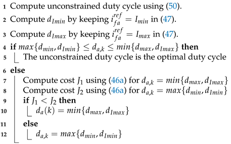
The unconstrained optimal duty cycle is obtained by differentiating (45a) with respect to d a , k . To obtain the optimal d a , k ,
J d a , k = 0
d a , k = v a n , k + 1 r e f + a 1 a n v a n , k + a 2 a n v a n , k 1 + a 3 a n v a n , k 2 b 2 a n ( d a , k 1 0.5 ) v d c b 1 a n v d c + 0.5
If d a , k satisfies (48), then (50) will be the optimal duty cycle. If  d a , k does not satisfy (48), then we need to compute d I m i n for I m i n and d I m a x for I m a x using (47). After this step, we need to compute the cost for m i n { d m a x , d I m a x } and m a x { d m i n , d I m i n } . The set that has minimum cost will be the optimal duty cycle. The proposed scheme to compute the optimal duty cycle is given in Algorithm 1. The proposed MFPC block diagram is shown in Figure 2.
Algorithm 1: Proposed model-free predictive control
Energies 17 03761 i001

6. Stability Analysis

The stability of model-free predictive control (MFPC) with constraints is a complex problem. This section explains the stability of unconstrained MFPC for phase A. The stability analysis for phases B and C will follow the same process. For convenience in stability analysis, we convert (39) into a state-space form with n A = 3 and n B = 2 .
x k + 1 = a 1 a n a 2 a n a 3 a n 1 0 0 0 1 0 x k + 1 0 0 ( d a , k 0.5 ) v d c v a n , k = b 1 b 2 0 x k + [ 0 ] ( d a , k 0.5 ) v d c
Using (46a) and (51), the optimal d a , k is
d a ( k ) = v a n , k + 1 r e f C B v d c k x ( k ) v d c + 0.5
with k = C A C B using optimal d a , k from (52) in (51), the closed-loop state-space model is defined as:
x k + 1 = a 1 a n a 2 a n a 3 a n 1 0 0 0 1 0 x k + 1 0 0 ( v a n , k + 1 r e f C B v d c k x ( k ) v d c + 0.5 0.5 ) v d c v a n , k = b 1 b 2 0 x k
The closed-loop state-space model in (53) is written as:
x k + 1 = A c l x k + B c l u v a n , k = C c l x k
with
A c l = A B c l k , B c l = B C B , C c l = C .
We used Lyapunov stability criteria to analyze the stability of the closed-loop system (51). The Lyapunov function is defined as
J a , k = ( v a n , k + 1 r e f v a n , k + 1 ) T ( v a n , k + 1 r e f v a n , k + 1 )
According to Lyapunov stability criteria, the following condition should satisfy:
j a , k j a , k 1 < 0
If u * is the optimal input for (54), then v a n , k + 1 r e f and v a n , k + 1 are defined as
v a n , k + 1 r e f = C a l A a l x k r e f + C c l B c l u *
v a n , k + 1 = C c l A c l x k + C c l B c l u *
j a , k + 1 = ( C c l A c l x k r e f + C c l B c l u * C c l A c l x k C c l B c l u * ) T ( C c l A c l x k r e f + C c l B c l u * C c l A c l x k C c l B c l u * ) = ( C A e k ) T C A e k
j a , k = ( v k r e f v k ) T ( v k r e f v k ) = ( C c l e k ) T ( C c l e k )
j a , k + 1 j a , k = e k + 1 T e k + 1 e k T e k = ( C A e k ) T C A e k e k T C c l T C c l e k
j a , k + 1 j a , k = e k T ( A c l T C c l T C c l C c l A c l T C c l T C c l ) e k
To satisfy the Lyapunov stability condition, the following condition is proposed:
( ( C c l A c l ) T C c l A c l C c l T C c l ) < 0
The eigenvalues of (63) are negative which proves that matrix ( ( C c l A c l ) T C c l A c l C c l T C c l ) is negative definite. This fulfills the Lyapunov stability condition (56). Hence, the closed-loop system (54) is asymptotically stable.

7. Results

This section presents simulation and high-fidelity model results to validate the performance of the proposed scheme. Two main scenarios are the performance of the MFPC in the presence of constraints on the filter current and duty cycle. The second scenario discusses the comparison of the proposed MFPC and MPC for a model mismatch.
The simulations have been performed in Matlab/Simulink. For high-fidelity model results, hardware in-loop (HIL) real-time simulations have been performed in Typhoon 604. The parameters for the experimental and simulation results have been shown in Table 1. The order of the polynomials A y ( z ) and B x ( z ) are n A = 3 and n B = 2 , respectively.

7.1. Steady State Performance

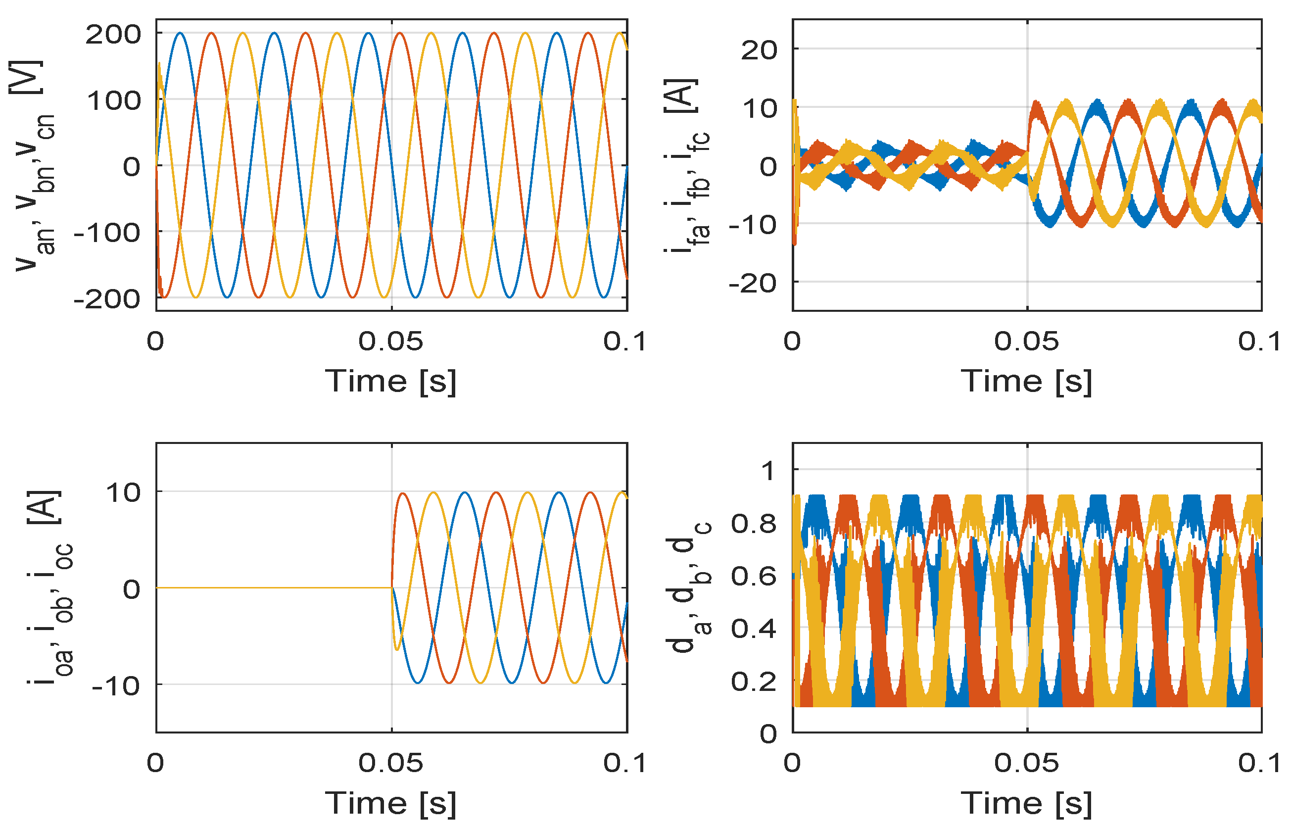
Figure 3 shows the simulation results of the proposed approach for an inductive load with L = 10 mH and R = 20 Ω . The inductive load turns on at 5 msec. The controller regulates the output voltages in the presence of the constraints. During the start time, the capacitor draws a large amount of current; as a result, there is some distortion in output voltages. However, due to constraints on the filter current, the controller limits the overshoot between I m a x and I m i n . The filter currents violate the constraints slightly because of the state-space average method that neglects the switching behavior [25].
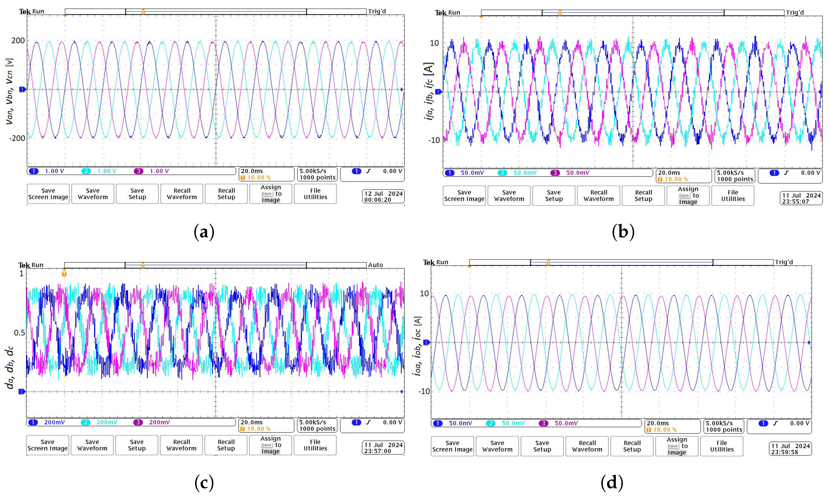
Figure 4 shows the HIL results of the proposed approach for an inductive load with L = 10 mH and R = 20 Ω . Figure 4a shows that the proposed approach regulates output voltages v a n , v b n , and v c n at the desired reference. Figure 4b shows that filter currents I f a , I f b and I f c remain within the constraints I m a x and I m i n . Moreover, Figure 4c shows that the optimal duty cycles d a , d b , and d c also remain within the constraints d m a x and d m i n . The inductive load currents i o a , i o b and i o c are shown in Figure 4d.

7.2. Model Mismatch Performance

Figure 5 shows the HIL results of the proposed MFPC and MPC for an ideal model or nominal values of L and C. The comparison of Figure 5a,b shows that for an ideal model, the performance of the proposed MFPC and MPC is similar.
Figure 6 shows the performance of the proposed MFPC and MPC for a change in the value of C by 30 percent while the value of L remains nominal. In this scenario, a comparison of Figure 6a,b shows that the proposed MFPC is still regulating the voltages. However, the MPC has a poor performance for change in the value of C.
Figure 7 shows the performance comparison of the proposed MFPC and MPC for a change in the value of L by 30 percent while the value of C remains nominal. Figure 6a,b show that the proposed MFPC gives much better output voltage compared to MPC.
Figure 8 shows the HIL results of the proposed MFPC and MPC for change in the value of L and C by 30 percent. A comparison of Figure 8a,b shows that the MFPC performance for regulating the output voltages is better than the MPC.

8. Converter Efficiency

The choice of switching frequency plays a crucial role in the converter’s efficiency. A higher switching frequency results in higher switching losses, and vice versa. To demonstrate the advantage of the proposed CCS-based MFPC, the efficiency of the inverter is computed for both the proposed MFPC and the FCS-MFPC [14]. Figure 9 shows the input and output power comparison of the inverter for the proposed MFPC and the FCS-MFPC. The efficiency of the inverter with the proposed MFPC and FCS-MFPC is η = 91 % and η = 86 % , respectively. This comparison shows that the proposed approach has fewer switching losses compared to FCS-MFPC and achieves an efficiency greater than 90 % .

9. Computational Efficiency

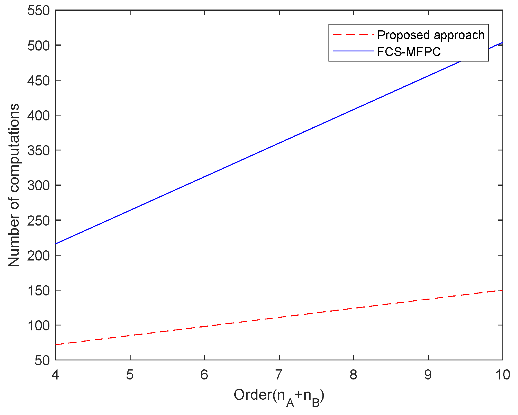
We used simple criteria for measuring the computational efficiency of the algorithm. In this criteria, we computed the number of computations of the algorithm when obtaining an optimal control action. We compared the computational efficiency of the proposed approach with the conventional FCS-MFPC [14]. The computations of the proposed approach and FCS-MFPC are summarized in Table 2. The computations of both algorithms for different values of the model order are shown in Figure 10. The proposed approach requires three times less computations than the FCS-MFPC for any value of n A and n B . Computational efficiency will help to operate the controller at a higher switching frequency and its implementation on low-cost hardware or a trade-off.

10. Conclusions

This paper has presented an improved CCS-MFPC for a three-phase inverter with an LC filter. Further, the paper has proposed a computationally efficient tailored active set method to solve the optimization problem of the MFPC. The constraints on the maximum admissible filter current and duty cycle are part of the control scheme. Due to the CCS nature which has a fixed switching frequency compared to FCS, the design of the output LC filter is an easy task. Moreover, the computational efficiency of the algorithm is three times compared to the conventional FCS-MFPC. This computational efficiency helps to operate the controller at a high switching frequency and implementation of the controller on low-cost digital hardware. Results have shown that the proposed controller regulates the output voltages subject to constraints on the duty cycle and filter current. Further, in case of a model mismatch, the overall performance of MFPC is much better compared to MPC.

Author Contributions

Conceptualization, M.N. and W.S.; methodology, M.N.; software, M.N.; validation, M.N.; formal analysis, M.N.; investigation, M.N.; resources, W.S.; data curation, M.N.; writing—original draft preparation, M.N.; writing—review and editing, M.N.; visualization, M.N.; supervision, W.S. All authors have read and agreed to the published version of the manuscript.

Funding

This research received no external funding.

Data Availability Statement

We are unable to share data due to privacy concerns.

Conflicts of Interest

There is no conflict of interest.

References

  1. Yang, Y.; Xiao, Y.; Fan, M.; Wang, K.; Zhang, X.; Hu, J.; Fang, G.; Zeng, W.; Vazquez, S.; Rodriguez, J. A novel continuous control set model predictive control for LC-filtered three-phase four-wire three-level voltage-source inverter. IEEE Trans. Power Electron. 2023, 38, 4572–4584. [Google Scholar] [CrossRef]
  2. Pirsto, V.; Kukkola, J.; Hinkkanen, M. Multifunctional cascade control of voltage-source converters equipped with an LC filter. IEEE Trans. Ind. Electron. 2021, 69, 2610–2620. [Google Scholar] [CrossRef]
  3. Xue, C.; Zhou, D.; Li, Y. Finite-control-set model predictive control for three-level NPC inverter-fed PMSM drives with LC filter. IEEE Trans. Ind. Electron. 2020, 68, 11980–11991. [Google Scholar] [CrossRef]
  4. Safamehr, H.; Najafabadi, T.A.; Salmasi, F.R. Adaptive control of grid-connected inverters with nonlinear LC filters. IEEE Trans. Power Electron. 2022, 38, 1562–1570. [Google Scholar] [CrossRef]
  5. Nauman, M.; Hasan, A. Efficient implicit model-predictive control of a three-phase inverter with an output LC filter. IEEE Trans. Power Electron. 2016, 31, 6075–6078. [Google Scholar] [CrossRef]
  6. Karamanakos, P.; Liegmann, E.; Geyer, T.; Kennel, R. Model predictive control of power electronic systems: Methods, results, and challenges. IEEE Open J. Ind. Appl. 2020, 1, 95–114. [Google Scholar] [CrossRef]
  7. Toso, F.; Favato, A.; Torchio, R.; Alotto, P.; Bolognani, S. Continuous control set model predictive current control of a microgrid-connected pwm inverter. IEEE Trans. Power Syst. 2020, 36, 415–425. [Google Scholar] [CrossRef]
  8. Bemporad, A. Explicit model predictive control. In Encyclopedia of Systems and Control; Springer: Cham, Switzerland, 2021; pp. 744–751. [Google Scholar]
  9. Nauman, M.; Shireen, W.; Hussain, A. Model-Free Predictive Control and Its Applications. Energies 2022, 15, 5131. [Google Scholar] [CrossRef]
  10. Saeed, J.; Wang, L.; Fernando, N. Model predictive control of phase shift full-bridge DC–DC converter using Laguerre functions. IEEE Trans. Control Syst. Technol. 2021, 30, 819–826. [Google Scholar] [CrossRef]
  11. Berberich, J.; Köhler, J.; Müller, M.A.; Allgöwer, F. Data-driven model predictive control with stability and robustness guarantees. IEEE Trans. Autom. Control 2020, 66, 1702–1717. [Google Scholar] [CrossRef]
  12. Ipoum-Ngome, P.G.; Mon-Nzongo, D.L.; Flesch, R.C.C.; Song-Manguelle, J.; Wang, M.; Jin, T. Model-free predictive current control for multilevel voltage source inverters. IEEE Trans. Ind. Electron. 2020, 68, 9984–9997. [Google Scholar] [CrossRef]
  13. Khalilzadeh, M.; Vaez-Zadeh, S.; Rodriguez, J.; Heydari, R. Model-free predictive control of motor drives and power converters: A review. IEEE Access 2021, 9, 105733–105747. [Google Scholar] [CrossRef]
  14. Rodriguez, J.; Heydari, R.; Rafiee, Z.; Young, H.A.; Flores-Bahamonde, F.; Shahparasti, M. Model-free predictive current control of a voltage source inverter. IEEE Access 2020, 8, 211104–211114. [Google Scholar] [CrossRef]
  15. Heydari, R.; Young, H.; Flores-Bahamonde, F.; Vaez-Zadeh, S.; Gonzalez-Castano, C.; Sabzevari, S.; Rodriguez, J. Model-free predictive control of grid-forming inverters with LCL filters. IEEE Trans. Power Electron. 2022, 37, 9200–9211. [Google Scholar]
  16. Wei, Y.; Young, H.; Wang, F.; Rodríguez, J. Generalized data-driven model-free predictive control for electrical drive systems. IEEE Trans. Ind. Electron. 2022, 70, 7642–7652. [Google Scholar] [CrossRef]
  17. Cheng, C.; Xie, S.; Qian, Q.; Xu, J.; Zeng, B.; Lv, J. On Stability of Time-Invariant Current Controlled Weak-Grid-Tied Inverters Considering Sinusoidal Pulsewidth Modulation Saturation and Parameter Uncertainties. IEEE Trans. Ind. Electron. 2022, 69, 11359–11369. [Google Scholar] [CrossRef]
  18. Van Waarde, H.J.; Eising, J.; Trentelman, H.L.; Camlibel, M.K. Data informativity: A new perspective on data-driven analysis and control. IEEE Trans. Autom. Control 2020, 65, 4753–4768. [Google Scholar] [CrossRef]
  19. Li, Y.R.; Peng, C.C.; Juang, J.N. An integral method for parameter identification of a nonlinear robot subject to quantization error. Nonlinear Dyn. 2023, 111, 22419–22441. [Google Scholar] [CrossRef]
  20. Schoukens, J.; Dobrowiecki, T.; Pintelon, R. Parametric and nonparametric identification of linear systems in the presence of nonlinear distortions-a frequency domain approach. IEEE Trans. Autom. Control 1998, 43, 176–190. [Google Scholar] [CrossRef]
  21. Kang, T.; Peng, H.; Xu, W.; Sun, Y.; Peng, X. Deep Learning-Based State-Dependent ARX Modeling and Predictive Control of Nonlinear Systems. IEEE Access 2023, 11, 32579–32594. [Google Scholar] [CrossRef]
  22. Brosch, A.; Hanke, S.; Wallscheid, O.; Böcker, J. Data-driven recursive least squares estimation for model predictive current control of permanent magnet synchronous motors. IEEE Trans. Power Electron. 2020, 36, 2179–2190. [Google Scholar] [CrossRef]
  23. Jiang, Shunhua and Natura, Bento and Weinstein, Omri, A faster interior-point method for sum-of-squares optimization. Algorithmica 2023, 85, 2843–2884. [CrossRef]
  24. Cimini, Gionata and Bemporad, Alberto Exact complexity certification of active-set methods for quadratic programming. IEEE Trans. Autom. Control. 2017, 62, 6094–6109. [CrossRef]
  25. Mariéthoz, S.; Morari, M. Explicit model-predictive control of a PWM inverter with an LCL filter. IEEE Trans. Ind. Electron. 2008, 56, 389–399. [Google Scholar] [CrossRef]
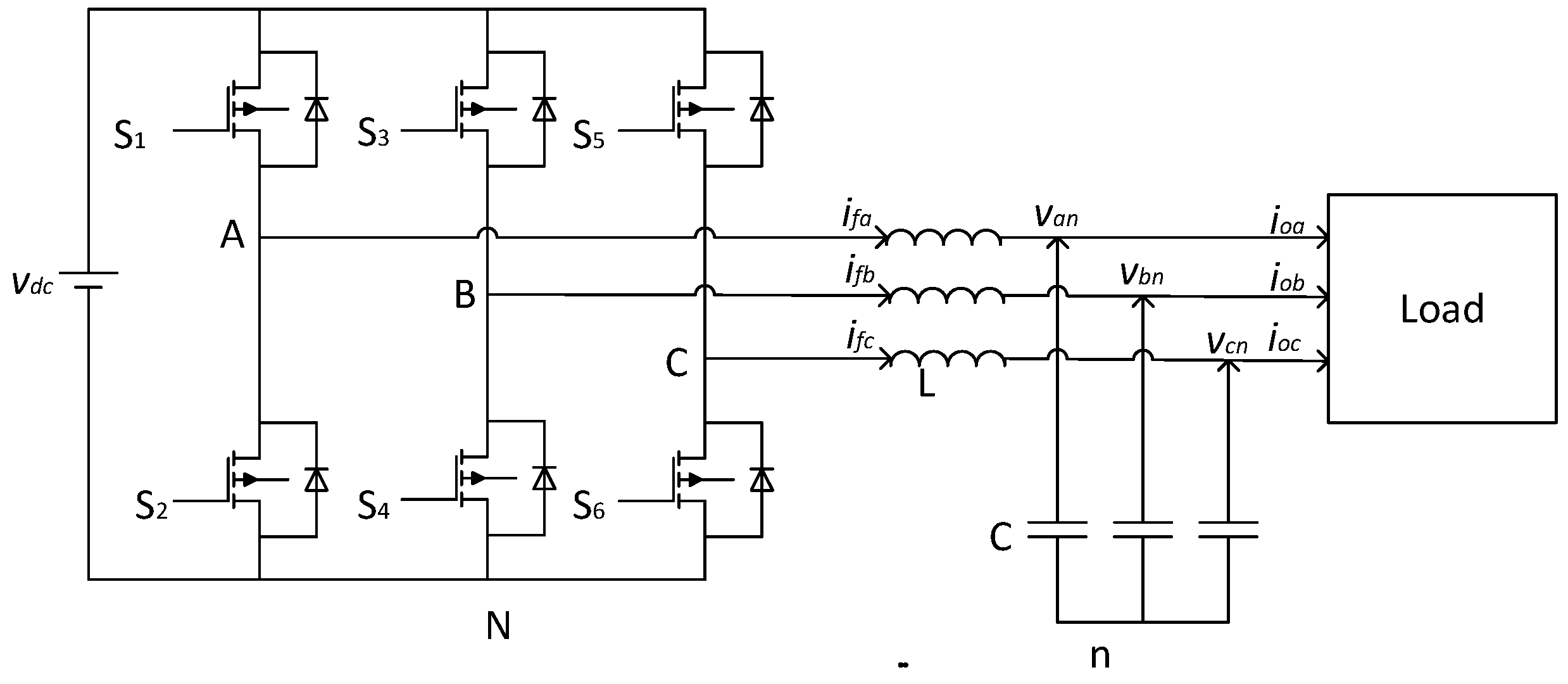
Figure 1. Three-phase inverter with LC filter.
Energies 17 03761 g001
Figure 2. Controller block diagram.
Energies 17 03761 g002
Figure 3. Simulation results of the proposed MFPC in the steady−state.
Energies 17 03761 g003
Figure 4. HIL result: Steady−state performance of the proposed MFPC. (a) Output voltages v a n ,   v b n ,   v c n . (b) Filter currents i f a ,   i f b ,   i f c . (c) Duty cycles d a ,   d b ,   d c . (d) Output currents i o a ,   i o b ,   i o c .
Energies 17 03761 g004
Figure 5. MPC and MFPC performance for Cx1 and Lx1.
Energies 17 03761 g005
Figure 6. MPC and MFPC performance for Cx0.3 and Lx1.
Energies 17 03761 g006
Figure 7. MPC and MFPC performance for Cx1 and Lx0.3.
Energies 17 03761 g007
Figure 8. MPC and MFPC performance for Cx0.3 and Lx0.3.
Energies 17 03761 g008
Figure 9. Input and output power of inverter for proposed MFPC and FCS-MFPC.
Energies 17 03761 g009
Figure 10. Computational comparison of proposed MFPC with FCS-MFPC.
Energies 17 03761 g010
Table 1. Parameters.
ParameterValue
Inductance of LC filter1 [mH]
Capacitance of LC filter40 [μF]
Sampling time Ts20 [μsec]
Inverter input DC voltage V s 520 [V]
Reference voltage200 [V]
Inductive load inductance10 [mH]
Inductive load resistance20 Ω
Maximum filter current I m a x 12 [A]
Minimum filter current I m i n −12 [A]
lambda ( λ )0.9
Table 2. Computations of the proposed MFPC and FCS-MFPC.
Algorithm × / ÷ +/−
Proposed MFPC 6 ( n A + n B + 1 ) 6 ( n A + n B + 2 )
FCS-MFPC 24 ( n A + n B + 1 ) 24 ( n A + n B )
Disclaimer/Publisher’s Note: The statements, opinions and data contained in all publications are solely those of the individual author(s) and contributor(s) and not of MDPI and/or the editor(s). MDPI and/or the editor(s) disclaim responsibility for any injury to people or property resulting from any ideas, methods, instructions or products referred to in the content.