Article

Long Short-Term Memory Autoencoder and Extreme Gradient Boosting-Based Factory Energy Management Framework for Power Consumption Forecasting

1
Department of Smart Factory Convergence, Sungkyunkwan University, 2066 Seobu-ro, Jangan-gu, Suwon 16419, Republic of Korea
2
Department of Bio-Mechatronic Engineering, Sungkyunkwan University, 2066 Seobu-ro, Jangan-gu, Suwon 16419, Republic of Korea
*
Author to whom correspondence should be addressed.
Energies 2024, 17(15), 3666; https://doi.org/10.3390/en17153666
Submission received: 1 July 2024 / Revised: 21 July 2024 / Accepted: 23 July 2024 / Published: 25 July 2024
(This article belongs to the Section A1: Smart Grids and Microgrids)

Abstract

:
Electricity consumption prediction is crucial for the operation, strategic planning, and maintenance of power grid infrastructure. The effective management of power systems depends on accurately predicting electricity usage patterns and intensity. This study aims to enhance the operational efficiency of power systems and minimize environmental impact by predicting mid to long-term electricity consumption in industrial facilities, particularly in forging processes, and detecting anomalies in energy consumption. We propose an ensemble model combining Extreme Gradient Boosting (XGBoost) and a Long Short-Term Memory Autoencoder (LSTM-AE) to accurately forecast power consumption. This approach leverages the strengths of both models to improve prediction accuracy and responsiveness. The dataset includes power consumption data from forging processes in manufacturing plants, as well as system load and System Marginal Price data. During data preprocessing, Expectation Maximization Principal Component Analysis was applied to address missing values and select significant features, optimizing the model. The proposed method achieved a Mean Absolute Error of 0.020, a Mean Squared Error of 0.021, a Coefficient of Determination of 0.99, and a Symmetric Mean Absolute Percentage Error of 4.24, highlighting its superior predictive performance and low relative error. These findings underscore the model’s reliability and accuracy for integration into Energy Management Systems for real-time data processing and mid to long-term energy planning, facilitating sustainable energy use and informed decision making in industrial settings.

1. Introduction

Electricity consumption significantly impacts the operation, strategic planning, and maintenance of power grid infrastructure. The efficiency and optimal performance of power systems are determined by electricity usage patterns and intensity, necessitating careful management [1]. The socioeconomic impacts of electricity usage are substantial, as it serves as a key driver of economic development by enabling industrial activities, commercial operations, and residential demand fulfillment. In the industrial sector, electricity powers machinery and manufacturing processes, promoting productivity and economic growth [2].
With the increasing demand for processing and analyzing vast amounts of data, big data analytics and machine learning-based predictive research have become prevalent. These methods are applied to analyze energy consumption patterns and forecast demand across various types of buildings, enhancing energy efficiency. Among these, the Factory Energy Management System (FEMS), an Energy Management System (EMS) applied to factories, is noteworthy. The FEMS monitors the energy consumption of factories comprehensively, analyzes the collected large-scale energy data, identifies equipment and utilities consuming energy during production downtime, and enables optimal control. This technology is recognized for its potential to reduce energy consumption in the industrial sector by balancing energy demand and supply, reducing unnecessary energy waste, addressing environmental issues, and cutting costs [3].
Electricity consumption predictions can be categorized into short-term, mid-term, and long-term, encompassing prediction periods of 24 h to a week, a week to a year, and over a year, respectively [4]. Different types of electricity forecasts serve various purposes. Short-term forecasts are used to provide the theoretical basis for hydropower generation scheduling and the startup and shutdown of equipment [5]. Mid-term forecasts rationalize the maintenance of grid equipment, while long-term forecasts are primarily used by grid planning departments for renovation and expansion plans [6]. The primary objective of this study is to enhance the prediction of mid-term power usage of industrial facilities, detect anomalies in energy consumption, and improve the operational efficiency of power systems while minimizing environmental impact.
Although existing models such as ARIMA and Exponential Smoothing are optimized for short-term forecasting, they often struggle with long-term predictions due to seasonality and non-stationarity in data, making them computationally intensive and less accurate in capturing long-term dependencies [7,8]. Furthermore, models like Prophet and GRU face challenges in effectively incorporating irregular patterns such as holidays and events into their forecasts. In contrast, our proposed model focuses on mid to long-term forecasting by leveraging an ensemble approach that combines a Long Short-Term Memory Autoencoder (LSTM-AE) with Extreme Gradient Boosting (XGBoost). This combination allows us to handle the complexities of long-term dependencies and non-linearities in data more effectively. Additionally, we introduce the use of Expectation Maximization Principal Component Analysis (EM-PCA) for data preprocessing, which optimizes the data by handling missing values and selecting important features, thereby reducing computational load and enhancing model efficiency.
This study introduces an innovative ensemble model combining LSTM-AE and XGBoost to precisely predict complex electricity usage patterns and address the computational inefficiencies of traditional models. The integration of these models enhances prediction accuracy, especially by incorporating critical socioeconomic variables such as System Marginal Price (SMP) and special event indicators that significantly impact consumption patterns. Data preprocessing involves EM-PCA [9] to handle missing values and feature selection, ensuring the robustness and reliability of the forecasts.
The major contributions of this study are as follows:
  • Superior predictive performance for mid to long-term forecasting: our method demonstrated significant improvements in various evaluation metrics compared to existing models, highlighting its capability in forecasting complex industrial energy systems over mid to long-term periods.
  • Enhanced handling of non-standard events: by integrating event indicators and SMP data, the model adeptly handles non-standard events and holidays, which are critical for accurate mid to long-term forecasting, traditionally a weak point in existing forecasting models.
  • Optimized data preprocessing: the application of EM-PCA not only improved the handling of missing data but also effectively managed feature extraction, which is critical for enhancing the predictive accuracy of complex models in mid to long-term scenarios.
The Introduction explains the background and objectives of the study, emphasizing its necessity and importance. It also briefly introduces the proposed methodology, dataset, and major contributions. The Related Work section discusses the importance of electricity consumption prediction, existing models, and their limitations, and it provides examples of the application of deep learning and ensemble models. The Methodology section details the structure of the proposed model, including the design and implementation of the ensemble approach. The Experiments and Results section presents the experimental setup and model training results, comparing the performance using various metrics. Finally, the Conclusion and Future Work section summarizes the main findings and contributions of the study, emphasizing its significance and suggesting future research directions.

2. Related Work

2.1. Energy Management in Smart Manufacturing

The core of the Fourth Industrial Revolution is the implementation of smart factories, which integrate IT systems into manufacturing processes [10]. Internet of Things (IoT)-based smart factories manage energy efficiently by collecting and sharing data from production machinery in real time. The FEMS operates in four primary stages. The first stage involves evaluating current energy management practices and defining improvement targets. The second stage collects and analyzes data in real time through IoT technology. The third stage integrates the collected data via an Energy Management System. In the fourth stage, strategies and action plans are developed to improve the energy efficiency of the smart factory [11]. Thus, the FEMS goes beyond data collection and analysis to comprehend energy flows in buildings, manufacturing systems, and processes [12].
In the context of buildings, the FEMS can utilize a hybrid AI-based framework that considers consumer behavior and weather conditions to provide accurate forecasts of power consumption and generation [13]. For instance, factories located in regions with high solar irradiance can achieve significant energy savings by reducing the use of lighting systems during daylight hours through the effective utilization of natural light [14]. In manufacturing systems, FEMS can employ an adaptive predictive controller based on dynamic energy models to manage the activation and deactivation of peripheral devices at optimal times [15]. This approach helps continuously update changes in energy consumption due to the natural degradation of industrial equipment, reducing discrepancies with actual energy usage. At the process level, FEMS can achieve energy optimization goals through energy-efficient scheduling based on multi-task and multi-resource scenarios [16].

2.2. Data Preprocessing in Forecasting

Data preprocessing transforms raw data into a format that is easier to handle. The method of preprocessing varies depending on the purpose of data processing and typically involves data cleaning, data integration, data reduction, and data transformation [17]. ‘Data cleaning’ involves identifying and modifying noise, missing values, and outliers [18]. Noise refers to unwanted interference in the signal, which can be addressed through methods such as binning, clustering, and regression [19]. Recently, autoencoders, a type of bottleneck artificial neural network, have been used to remove noise [20]. Missing values occur when specific data values are absent, which can be due to loss, the absence of the attribute for an instance, or the observer’s disregard for the attribute’s importance [18]. Methods to handle missing values include (1) ignoring instances with unknown attributes, (2) selecting the most common attribute value, (3) substituting with the mean, (4) using regression or classification methods, and (5) treating missing values as special values [21]. Outliers are observations significantly deviating from other data points and can be detected using normalization, Z-Score, and Interquartile Range. Visual inspection is often preferred for detecting outliers as traditional methods might not be applicable depending on the data characteristics [22]. Detected outliers can be replaced with upper or lower bounds or mean values, considering the data’s nature [23].
‘Data integration’ transforms data from various sources into a single format, while ‘data reduction’ reduces data size to facilitate effective analysis. Discretization algorithms convert continuous data into discrete data, resulting in reduced data size [24]. These algorithms are classified into top-down and bottom-up approaches. The top-down approach starts with broad intervals and recursively partitions into smaller intervals. The bottom-up approach begins with single-value intervals and iteratively merges neighboring intervals [24]. Other methods include error-based and entropy-based partitioning [25]. ‘Data transformation’ modifies data’s format or structure, using normalization methods like Min-Max and Z-Score normalization to adapt the data to different structures [26].

2.3. Prediction Horizons

Based on different time scales, predictions can be categorized into various horizons. These range from very short-term scenarios, with predictions typically under 30 min, to long-term predictions extending up to a month. The development of forecasting methods has progressed significantly over the past decade, benefiting from advancements in high-performance computing tools and the establishment of increasingly sophisticated computational methods. Depending on different functional requirements, predictive horizons can be divided into four major time scales, as summarized in Table 1. It is important to note that forecasting errors tend to increase as the time horizon extends [27].

2.4. Time Series Forecasting Models

Accurately predicting electricity consumption is challenging due to various influencing factors such as population size, economic development, power infrastructure, and climatic conditions. The most widely used electricity load forecasting models can be categorized into three types: statistical models, machine learning models, and hybrid models [29]. Prediction models based on linear regression require a large number of training samples and tend to accumulate errors during the training process [30]. Additionally, linear regression models cannot update data characteristics or automatically correct biases, making them less suitable for proposing electricity consumption forecasting models [31]. Our focus is on machine learning models and hybrid models. Deep learning methods offer advantages such as autonomous feature extraction, high accuracy, strong learning capability, and generalizability. These advantages have led to the adoption of deep learning for proposing electricity consumption forecasting models. Key algorithms used for electricity consumption forecasting include CNN [32], LSTM [33], RNN [34], LightGBM [35], and Prophet [36]. LightGBM is a gradient boosting framework that uses tree-based learning algorithms, making it particularly efficient for large datasets and high-dimensional data [35]. Prophet, developed by Facebook, is a time series forecasting tool that handles missing data and trend changes effectively [36]. Another noteworthy algorithm is GGNet, which introduces a novel graph structure for power forecasting in renewable power plants, effectively considering temporal lead–lag correlations [37]. GGNet leverages the inherent temporal and spatial dependencies in power data to improve forecasting accuracy.
Deep learning-based electricity consumption forecasting models require large amounts of data samples for rolling training to achieve accurate predictions. However, as the number of prediction steps increases, bias in the prediction results also increases. For instance, an ED-Wavenet-TF-based wind energy prediction model showed increasing prediction errors as the prediction steps increased from 1 to 4 [38]. Deep learning-based electricity consumption forecasting models cannot fully resolve the issue of misinterpretation. Therefore, improving the accuracy of industrial electricity consumption forecasting models is a crucial factor in achieving the practical application of these models [31]. Even when machine learning methods address these non-linear interactions and generate better predictions, overfitting remains an issue with high-dimensional data. Recently, various deep learning models and their hybrid versions have been developed for power load forecasting, showing better results compared to traditional machine learning methods [6]. Zheng et al. [39] proposed a general framework for short-term load forecasting (STLF) combining Empirical Mode Decomposition, LSTM neural networks, and XGBoost with k-means clustering. To validate the performance of the proposed STLF framework, simulation experiments were conducted using hourly load data from New England-ISO. Lin et al. [40] also contribute to this field with a study focused on short-term electric load forecasting. At the core of their approach is the integration of variational mode decomposition and extreme learning machines to handle the non-linear nature of electric load data, which improves forecast reliability and accuracy, enabling more robust forecasts under the typical fluctuating environment of electric load data. Additionally, Tan et al. [41] proposed a multi-node load forecasting method based on multi-task learning with modal feature extraction, demonstrating significant improvements in prediction accuracy for complex power systems.

3. Materials and Methods

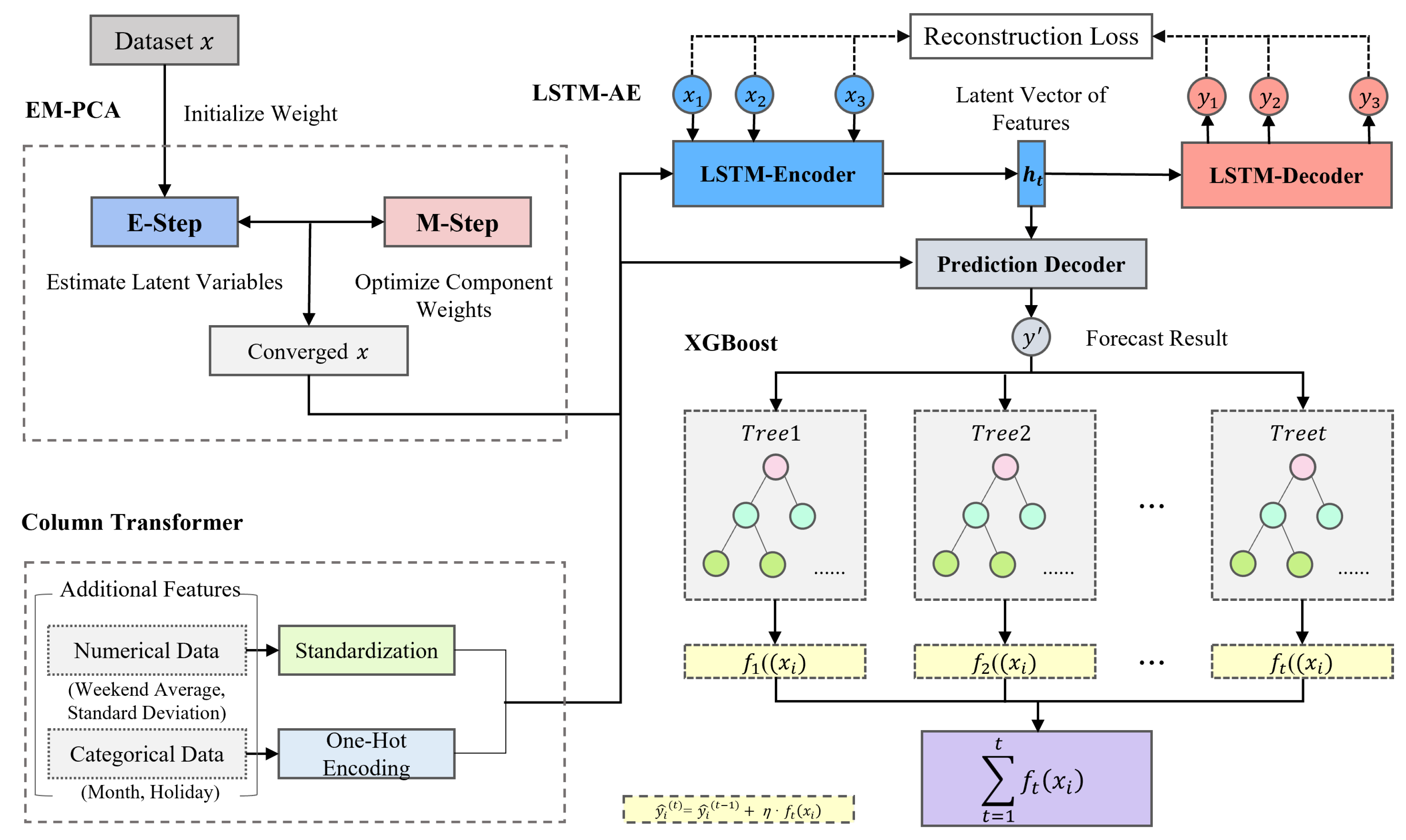
In this study, we propose an advanced approach for accurately predicting the power consumption of process equipment by ensembling advanced deep learning algorithms, LSTM-AE [42] and XGBoost [43]. This method enhances the precision and responsiveness of power management by better understanding and predicting the complexity of power consumption patterns compared to conventional single-model approaches. To illustrate the data preprocessing and model ensembling process for predicting power consumption in manufacturing plants, we present Figure 1, which visually represents the overall process of our research.
The first step involves the collection of input data. This study utilizes three main types of data: manufacturing power consumption data, system demand load data, and SMP data. The second step is data preprocessing and feature engineering. In this stage, raw data are transformed into an analyzable format, including handling missing values and removing outliers if necessary. Additionally, supplementary features such as weekend standard deviation and average are generated to enhance model performance. The third step is model ensembling. This stage aims to achieve optimal predictive performance by combining two primary models, LSTM-AE and XGBoost. The rationale for combining LSTM-AE and XGBoost lies in leveraging the strengths of both models: LSTM-AE’s ability to capture and extract significant features from time series data and XGBoost’s strength in handling structured data and performing feature importance analysis. LSTM-AE is used to extract significant features from time series data, providing a robust representation of the data. XGBoost is then employed for further feature engineering and hyperparameter tuning to achieve optimal performance. By integrating these models, we can utilize the temporal feature extraction capability of LSTM-AE and the powerful boosting technique of XGBoost to enhance overall model accuracy. The fourth step is forecasting. The final ensemble model, combining LSTM-AE and XGBoost, is used to perform the predictions and improve accuracy. The last step is performance evaluation. The predictive model’s performance is assessed using various evaluation metrics.
Our methodology systematically explains the process of data preprocessing, model ensembling, and performance evaluation to accurately predict the power consumption of manufacturing plants. Through this process, we develop a real-time prediction model that can be integrated into the FEMS of manufacturing plants, promoting sustainable energy use. Figure 2 illustrates the overall structure of the proposed model. It shows the feature extraction using LSTM-AE and feature importance evaluation using XGBoost. The extracted features are then used for XGBoost regression analysis, evaluating the importance of each feature. This process helps in selecting the most influential features for the predictive model.

3.1. Data Preprocessing in Smart Manufacturing

Data preprocessing is a critical step in this study, aiming to maximize the accuracy and efficiency of the model. The analysis phase for data preprocessing involves conducting Exploratory Data Analysis to understand the characteristics of the collected data, including patterns, missing values, outliers, and basic statistics. During data preprocessing, various power consumption data, such as real-time power consumption, historical consumption patterns, and peak consumption times, are analyzed and refined. This process includes handling missing values, normalization, feature extraction, and selection to create data suitable for modeling. Key statistical features are extracted during this phase, which provide crucial information for the model to learn the basic trends, seasonality, and periodicity of the time series data.

3.1.1. Key Variables and Feature Setting

We conduct data analysis to set the variables for forecasting power consumption in the forging process. The collected data include information for examining Demand Response (DR), system load data for the entire industry, and additional DR participation times. The DR Information Dataset contains data on DR programs, where electricity consumers adjust their usage to manage the power system load, balancing power demand and supply. This dataset includes data on each factory’s DR capacity, DR event dates, and start and end times, with DR capacity indicating the maximum power reduction achievable by participating in DR programs during peak times. System load represents the total amount of electricity used by manufacturing plants in Korea [44]. These data are crucial for analyzing the power consumption patterns of factories and their participation in DR programs. Thus, we included system load as a variable to understand power consumption patterns. Additionally, we included the SMP variable provided by the Korea Power Exchange [45]. SMP represents the marginal price of electricity when purchasing or selling power in the market, determined by supply and demand conditions. This price is used for transparent and fair pricing in the electricity market, with the highest-cost power plant setting the market price. These data are used in transactions between power generators and wholesale market participants. Since price factors are sensitive to changes in market demand and supply, SMP was included as an important variable for consumption forecasting.

3.1.2. Handling Missing Values and Outliers

We analyzed the basic structure and content of the data to identify missing values and outliers, verifying the basic statistical measures (mean, standard deviation, etc.) and the number of missing values in each column. We then extracted new columns (Year, Month, Day, Week) from the Date column. For analyzing patterns by month, day of the week, and time of day, we converted the Time column to datetime format and added variables for the daily average and standard deviation by day of the week.

3.1.3. Data Preprocessing Optimization Using EM-PCA

During the preprocessing stage, EM-PCA [9] was used to accurately estimate missing values and select significant features, reducing dimensionality. EM-PCA leverages temporally adjacent data to consider temporal change patterns, effectively extracting important information while maintaining data structure. Initially, only data with missing values are selected, and the weights for missing values are set to 0. The results are then updated in the original data frame, replacing the missing values with the estimated values.
X ^ m = P P T X o
P = arg max P X P P T X F 2
EM-PCA, an extension of Principal Component Analysis for incomplete datasets, uses the expectation-maximization algorithm to estimate principal components in data with missing values. The steps of EM-PCA are as follows:
  • Initialization: provide initial estimates for missing data X, filling missing values with initial means or medians and performing initial principal component estimates.
  • Application of EM-PCA: use EM-PCA to handle missing data, reducing dimensionality while preserving key characteristics.
  • Feature extraction: extract important features from the reduced-dimensionality data for use in the modeling phase.
  • E-step (expectation step) (1): calculate the expected values of missing data given the current principal component estimates.
  • M-step (maximization step) (2): Use the complete data calculated in the E-step to re-estimate the principal components. Repeat E-step and M-step until convergence, producing an optimal dataset with imputed missing values.
EM-PCA extracts principal components from data with missing values, effectively reducing dimensionality and retaining significant features. The principal components derived from this process capture the main variability of the data while minimizing the impact of missing values.

3.1.4. Feature Extraction Preprocessing

Using the extracted features, we construct a predictive model combining LSTM-AE [42] and XGBoost [43]. This process is conducted as follows. Numerical and categorical features are separated and preprocessed accordingly.
Numerical data preprocessing: (3) numerical data are standardized using StandardScaler, which adjusts each feature’s mean to 0 and standard deviation to 1.
z = x μ σ
where x represents the original data, μ is the mean, and σ is the standard deviation.
Categorical data preprocessing: categorical data are one-hot encoded using OneHotEncoder, converting categorical variables into a form that could be provided to ML algorithms to perform better in prediction. This transforms categorical variables into binary indicator variables, creating one field for each category, marked as 1 if the instance belongs to that category and otherwise 0. This conversion makes categorical data understandable for machine learning algorithms. The preprocessing pipeline is constructed using ColumnTransformer, which allows different transformations for numerical and categorical data. This transformer applies standardization to numerical data and one-hot encoding to categorical data, merging the results into a single dataset for modeling.

3.2. LSTM-AE and XGBoost Model Ensemble

3.2.1. Feature Extraction Using Long Short-Term Memory Autoencoder Model

LSTM-AE combines the LSTM and Autoencoder models to extract and reconstruct patterns from time series data. The upper right section of Figure 2 illustrates the structure of LSTM-AE. An Autoencoder is a deep neural network designed to reconstruct its input through encoding and decoding processes. The encoder compresses the input into a latent space representation, while the decoder reconstructs the original input from the encoded representation. LSTM networks are capable of retaining information from previous time steps and updating internal memory cells at each time step, allowing them to understand temporal relationships in data. The architecture of LSTM includes input, output, forget gates, and candidate memory cells. These components help the network learn, retain, or discard temporal relationships in the data, aiding the model’s learning process.
LSTM-AE enhances the accuracy of power consumption forecasting by better understanding and predicting the complex patterns in time series data. It is particularly useful for recognizing and forecasting temporal patterns in data. The LSTM-Encoder compresses the input sequence into a lower-dimensional representation, utilizing gating mechanisms to control the flow of information through recursive transformation processes [46].
f t = σ ( W f · [ h t 1 , x t ] + b f )
i t = σ ( W i · [ h t 1 , x t ] + b i )
o t = σ ( W o · [ h t 1 , x t ] + b o )
c t = f t c t 1 + i t tanh ( W c · [ h t 1 , x t ] + b c )
h t = o t tanh ( c t )
where σ represents the sigmoid activation function, h represents the hidden state, c represents the cell state, and f , i , and o denote the forget, input, and output gates, respectively. W and b represent the weights and biases for each gate. The LSTM-Decoder reconstructs the original input sequence from the encoded state, minimizing reconstruction loss. The Prediction Decoder uses the latent representation learned by the encoder to predict future values.

3.2.2. Prediction Using Extreme Gradient Boosting Model

The extracted features are fed into the XGBoost model to perform the final prediction. XGBoost is an enhanced version of gradient boosting, offering high predictive performance. It provides functionalities such as feature selection, automatic tree growth, and parallel processing per boosting round, enabling efficient training and prediction. XGBoost is resilient to overfitting and offers various hyperparameter tuning options to optimize the model [43]. The mechanism of XGBoost is as follows: Initially, a simple model (decision tree) is used to identify patterns in the training data. A new model is then added to minimize the errors of this initial model. This new model assigns higher weights to the samples that were incorrectly predicted by the previous model. This process is repeated, combining multiple decision trees to form a more robust ensemble model. For a given set of features X and results Y, the model sequentially builds trees, with each tree being trained to correct the errors of the previous trees. The update rule is as follows:
y ^ i ( t ) = y ^ i ( t 1 ) + η · f t ( x i )
where y ^ i ( t ) is the prediction at the t iteration, η is the learning rate, and f t is the function represented by the tree added at the t iteration.
Our models utilize established methodologies validated through previous research. For LSTM-AE, the training approach follows the general method of training LSTM neural networks, which is well documented in the literature. The process involves feeding time series data into the model and using backpropagation through time to update weights iteratively, minimizing the loss function. This allows the model to learn temporal dependencies effectively. Specifically, we referred to the detailed training techniques which highlight the use of CNN and LSTM autoencoders for short-term power generation forecasting [46]. For XGBoost, we adopted the framework described by Chen and Guestrin [43]. XGBoost builds an ensemble of trees sequentially, where each tree is trained to correct the residuals of the previous ones. This iterative boosting process enhances the model’s accuracy and robustness. The model’s hyperparameters were fine-tuned to optimize performance for power consumption forecasting, ensuring it captures the complex patterns in the data [43].
In terms of ensemble learning, our proposed method combines LSTM-AE and XGBoost to leverage the strengths of both models. LSTM-AE is used for feature extraction, capturing intricate temporal patterns in the data, while XGBoost utilizes these features for final prediction, enhancing the overall forecasting accuracy. This approach is based on the principle of ensemble learning, which combines multiple models to improve generalization and robustness [47].

3.2.3. Hyperparameter Tuning

Table 2 details the hyperparameters configured for the LSTM-AE model, crucial for capturing time series dependencies and preventing overfitting. This setup ensures the model learns effectively from the data while maintaining computational efficiency.
Table 3 presents the optimized hyperparameters for the XGBoost model, selected to maximize prediction accuracy and handle large-scale data effectively. These settings are determined to be the most effective after rigorous testing.
The process of hyperparameter tuning is crucial for optimizing machine learning models, ensuring they perform with high accuracy and efficiency. In this study, we employed RandomizedSearchCV to fine-tune the hyperparameters of the XGBoost model, aiming to enhance its predictive performance on the dataset. The pseudocode for this tuning process is illustrated in Algorithm 1.
Algorithm 1 Hyperparameter tuning using RandomizedSearchCV
  1:
Define hyperparameter ranges:
  2:
    n _ e s t i m a t o r s : [100, 200, 300, 500]
  3:
    m a x _ d e p t h : [3, 5, 7, 10]
  4:
    l e a r n i n g _ r a t e : [0.01, 0.05, 0.1, 0.2]
  5:
    s u b s a m p l e : [0.6, 0.8, 1.0]
  6:
    c o l s a m p l e _ b y t r e e : [0.6, 0.8, 1.0]
  7:
    r e g _ a l p h a : [0, 0.1, 0.5, 1]
  8:
    r e g _ l a m b d a : [0.1, 0.5, 1]
  9:
Configure RandomizedSearchCV:
10:
    estimator: XGBoost model
11:
    param_distributions: defined hyperparameter ranges
12:
    n_iter: 50
13:
    scoring: ‘neg_mean_absolute_error’
14:
    cv: 3
15:
    verbose: 2
16:
    random_state: 42
17:
    n_jobs: −1
18:
Fit RandomizedSearchCV with training data
19:
Return the best hyperparameters:
20:
    s u b s a m p l e : 0.8, r e g _ l a m b d a : 1, r e g _ a l p h a : 1, n _ e s t i m a t o r s : 300, m a x _ d e p t h : 7, l e a r n i n g _ r a t e : 0.05, c o l s a m p l e _ b y t r e e : 1.0
We defined the hyperparameter ranges that significantly impact the model’s performance. These included the number of estimators ranging from 100 to 500, the maximum depth of trees ranging from 3 to 10, the learning rate ranging from 0.01 to 0.2, the subsample ratio ranging from 0.6 to 1.0, the column sample by tree also ranging from 0.6 to 1.0, the regularization alpha ranging from 0 to 1, and the regularization lambda ranging from 0.1 to 1. The RandomizedSearchCV configuration was then set with the following parameters: the estimator was the XGBoost model; the parameter distributions were the predefined hyperparameter ranges; the number of iterations was set to 50 to specify the different combinations of hyperparameters to be tested; the scoring metric was neg_mean_absolute_error since Symmetric Mean Absolute Percentage Error (SMAPE) cannot be directly used with RandomizedSearchCV and Mean Absolute Error(MAE) serves as a close proxy; the cross-validation was set to 3-fold to ensure robust evaluation of model performance; verbosity was set to 2 to provide detailed logs during execution; the random state was set to 42 to ensure the reproducibility of the results; and the number of jobs was set to −1 to utilize all available processors for parallel execution.
Following this configuration, RandomizedSearchCV was fitted with the training dataset X train and the corresponding target values Y train. This process iterated over the defined hyperparameter space, evaluating each combination’s performance using the specified scoring metric and cross-validation strategy. The outcome of this fitting process was the identification of the best hyperparameters, which were then used to configure the final model for predictions. These parameters have proven to significantly improve the model’s performance, optimizing both accuracy and computational efficiency. This method efficiently and effectively searched across a wide hyperparameter space, balancing the trade-off between computational cost and model performance, thereby enhancing the model’s generalization ability from training data to unseen validation data.

4. Experiment and Results

4.1. Experimental Environment

The experimental environment used in this study is as follows. Table 4 shows the main hardware and software specifications used in the experiment. The CPU is a 13th Gen Intel(R) Core(TM) i9-13900KF 3.00 GHz, which performs complex calculations and data processing tasks quickly with its high-performance multi-core processor. The GPU utilized is an NVIDIA GeForce RTX 4090, which significantly enhances the training and inference speed of deep learning models, making it suitable for AI model training. The system also includes 64.0 GB of RAM, supporting the processing of large datasets and execution of complex algorithms. The software specifications used in the experiment are as follows: the operating system is Windows 11 Pro. Python version 3.8.10 is used for module compatibility, and PyCharm 2023.3.2 is employed as the development environment, providing an intuitive environment for efficient code development and debugging. PyTorch version 1.13.0+cu116 is used to optimize model development and training. TensorFlow version 2.13.0 is utilized, offering a flexible platform that supports various machine learning algorithms and models.

4.2. Dataset

The dataset used in this experiment comprises electricity consumption data collected every minute for seven months, from 1 March 2019 to 30 September 2019, from some manufacturing plants participating in the domestic DR market. Each plant exhibits approximate periodicity according to its manufacturing process. Plants implementing automated processes consistently recorded electricity consumption even during holidays. The power consumption of the plants varied according to their scale. Despite the limitation of the seven-month acquisition period, the weekly usage characteristics were strongly identified [44].
In this experiment, the power consumption datasets of the forging process from two plants were used. To predict the power consumption of the forging process, the power consumption data measured simultaneously from the two forging plants were extracted and merged into a single dataset. First, the data variables were merged into a single file according to the time, with the system demand collected in 5 min intervals and the forging power consumption in 1 min intervals, resampling the gaps between variables. Additionally, holiday and weekly average and standard deviation values were added as variables to create a data frame. To analyze data preprocessing, the distribution of columns in the Forge1 and Forge2 data was visualized, confirming that the power consumption patterns of the two processes were similar, as shown in Figure 3.
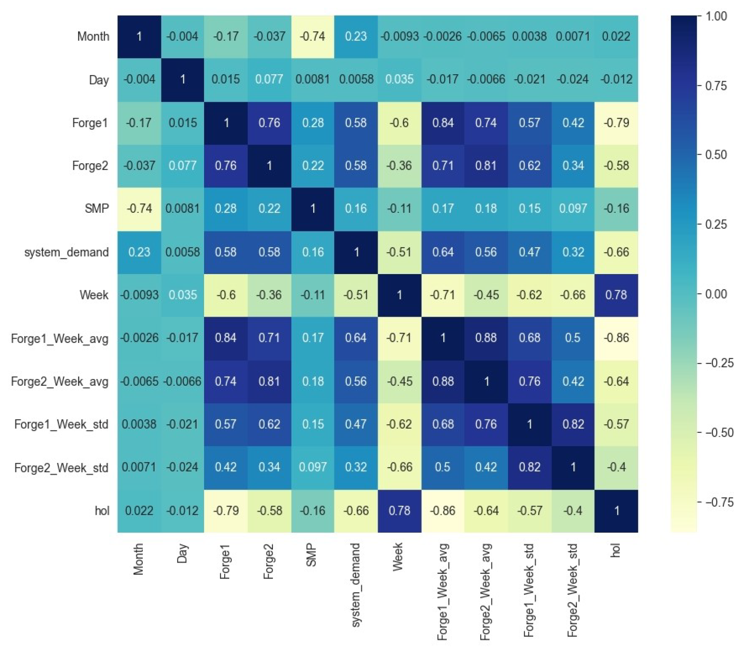
To select meaningful variables, the correlations between variables were examined through a correlation map, as shown in Figure 4. Forge1 and Forge2 (0.76) showed a high positive correlation, indicating that when the power consumption of Forge1 is high, the power consumption of Forge2 tends to be high as well. SMP and system demand (0.16) showed a slight positive correlation, suggesting that when power demand is high, the market price of power may increase, although the impact is not significant. System demand and Forge1 Weekly Standard Deviation ( 0.62 ) and Forge2 Weekly Standard Deviation ( 0.66 ) showed a strong negative correlation between system power demand and the weekly power consumption standard deviation of each Forge, indicating that the higher the power demand, the lower the variability in weekly power consumption. Forge1 Weekly Average and Forge2 Weekly Average (0.88) showed a very high positive correlation between the weekly average power consumption of the two Forges, indicating that when the weekly average consumption of one Forge is high, the other Forge shows a similar trend. Lastly, the holiday variable holiday and Forge2 Weekly Standard Deviation ( 0.58 ) and Forge2 Weekly Average (0.86) showed strong negative and positive correlations, respectively, between holidays and the weekly standard deviation and average of Forge2, suggesting that the variability in power consumption of Forge2 is lower and the average consumption is higher during holidays.
Based on Figure 5, the selected variables were used to create a new data frame, and the dataset was split into training data and validation data as shown in Figure 5a,b. The Validation Dataset was set to the power consumption from 1 September 2019 to 30 September 2019.

4.3. Performance Metrics

This study aims to enhance the accuracy of power consumption forecasting compared to existing models, reduce the error rate in anomaly detection in power consumption, and accurately quantify the environmental impact of energy consumption. The following performance metrics are used to evaluate the accuracy of the model. The performance metrics include MAE, Mean Squared Error (MSE), Coefficient of Determination (R2), and SMAPE to evaluate the accuracy of the predictive model.
MAE represents the mean of the absolute differences between actual and predicted values, with lower values indicating better accuracy.
MAE = 1 n i = 1 n | y i y ^ i |
MSE is the mean of the squared differences between predicted and actual values, indicating the size of the prediction error. Lower MSE values indicate higher predictive accuracy.
MSE = 1 n i = 1 n ( y i y ^ i ) 2
R2 indicates how well the model explains the actual values, ranging from 0 to 1, with values closer to 1 indicating better explanatory power. where y ¯ is the mean of the actual values.
R 2 = 1 i = 1 n ( y i y ^ i ) 2 i = 1 n ( y i y ¯ ) 2
SMAPE represents the mean of the absolute percentage differences between the predicted and actual values. It ranges from 0% to 200%, with lower values indicating higher predictive accuracy. Here, y i is the actual value and y ^ i is the predicted value.
SMAPE = 100 n i = 1 n | y i y ^ i | ( | y i | + | y ^ i | ) / 2

4.4. Experimental Results

The experimental process is as follows. First, the data variables were merged into a single file according to the time, with the system demand collected in 5 min intervals and the forging power consumption in 1 min intervals, resampling the gaps between variables.
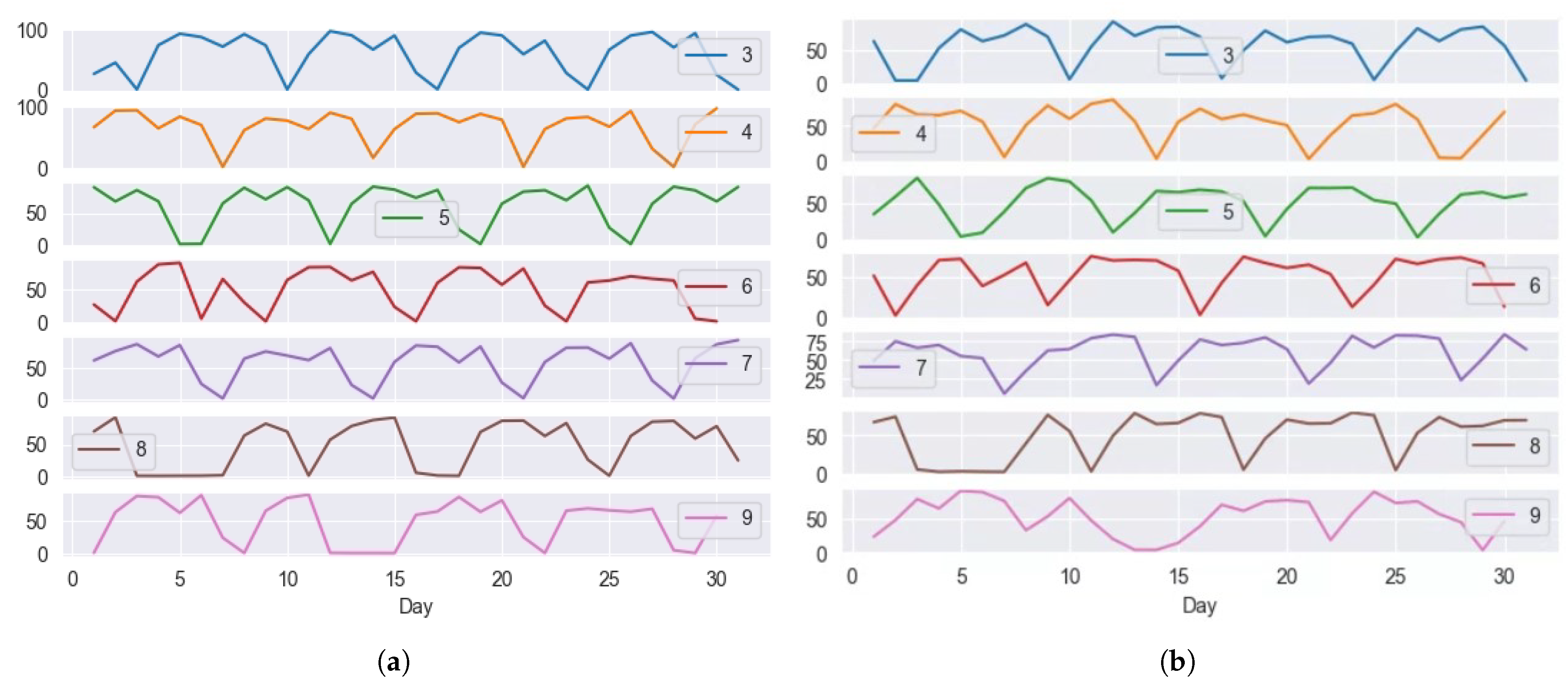
To examine the monthly distribution, the monthly power consumption of Forge1 and Forge2 was checked. Figure 6a,b show the trend of monthly power consumption for data preprocessing. Additionally, the generated data frame’s missing values and outliers were checked. Quantitative methods were not used to check for missing values, but qualitative methods such as graphs were used for confirmation.
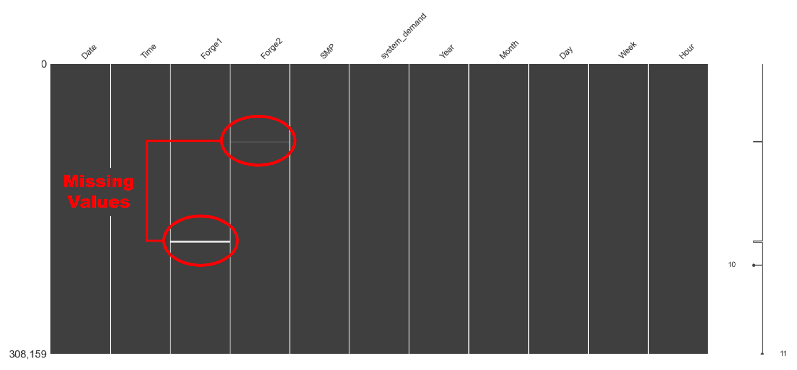
Figure 7 shows a qualitative visualization of missing data using Missingno Library: Forge1 had missing values on 9, 10, and 27 July, while Forge2 had a missing value on 27 April. Additionally, in this experiment, a DR event occurred temporarily from 18:00 to 19:00 on 13 June 2019, and this time was considered an outlier and preprocessed using the EM-PCA technique. The preprocessing results are shown in Figure 8.
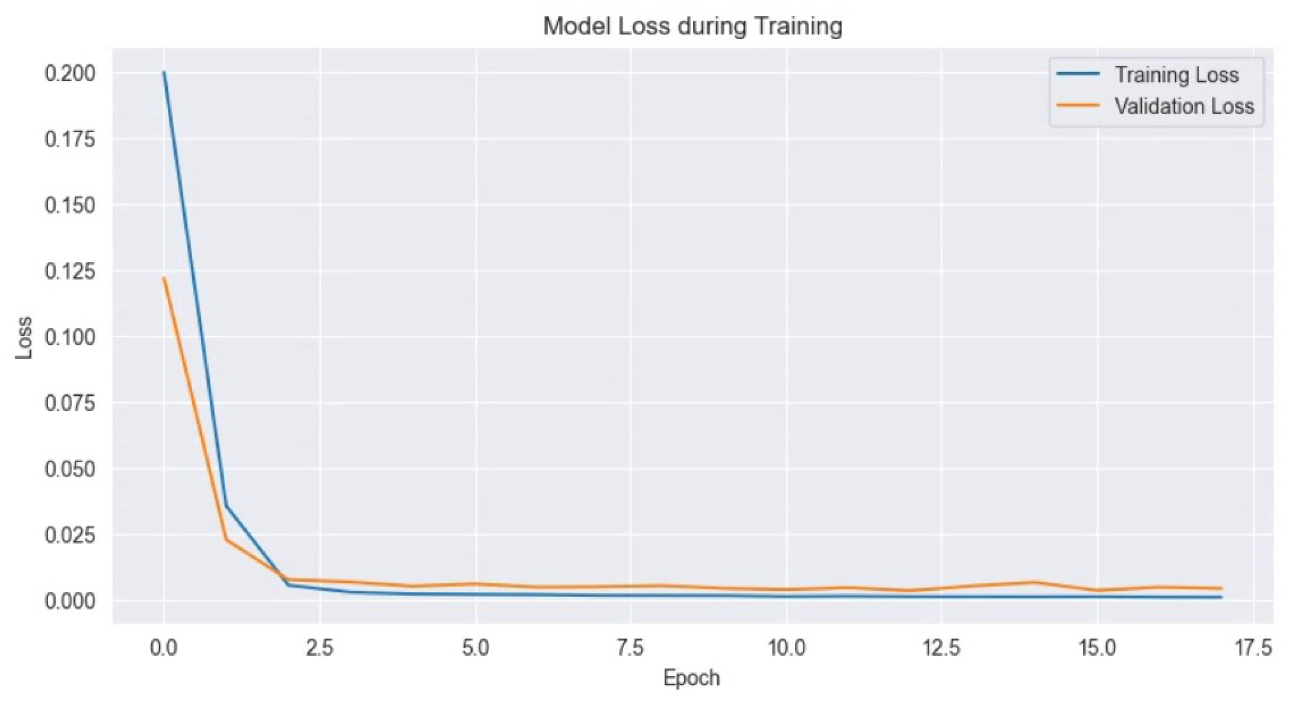
Figure 9 and Figure 10 show the results of applying the extracted features from LSTM-AE and additional variables to XGBoost training. Figure 9 visualizes the training and validation loss during feature extraction using the LSTM-AE model. The x-axis represents the number of epochs, and the y-axis represents the magnitude of loss. The training loss represents the loss on the training data, which decreases rapidly as epochs progress and stabilizes after a few epochs, indicating that the model adapts well to the training data. The validation loss represents the loss on the validation data, showing a similar trend to the training loss, stabilizing as epochs progress, indicating that the model maintains generalization performance without overfitting.
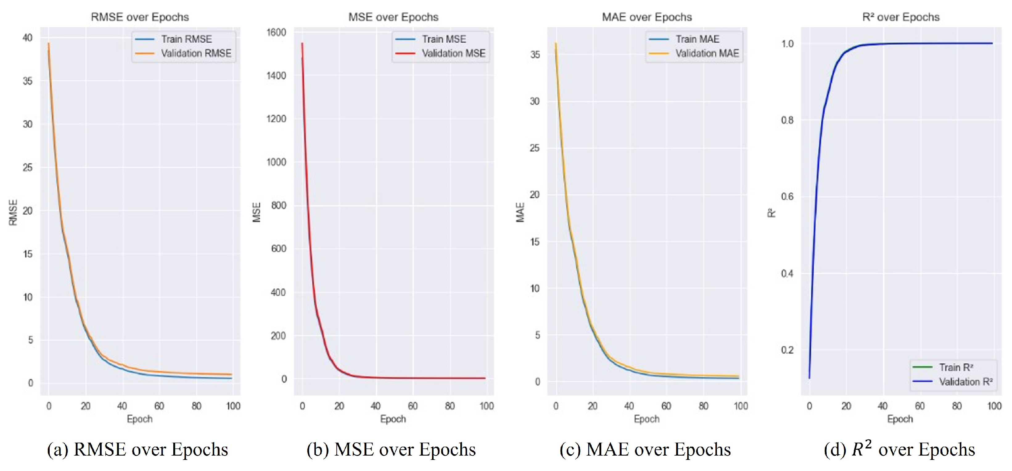
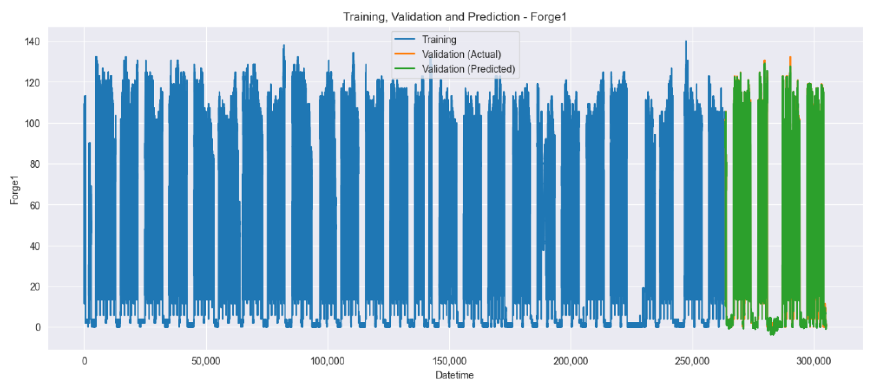
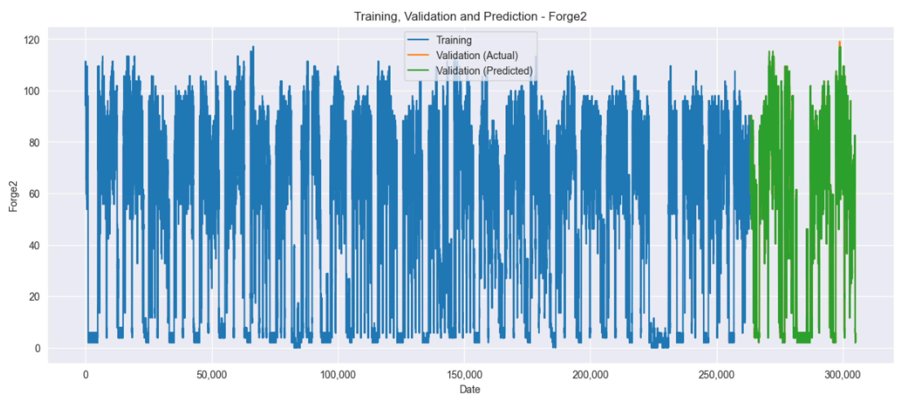
The graph in Figure 10 shows that the metrics for both the training and validation data are very similar, indicating no signs of overfitting. Specifically, the values for (a) RMSE, (b) MSE, (c) MAE, and (d) R2 consistently decrease or increase for both training and validation data. These results suggest that the model generalizes well to both training and validation data. In both graphs, blue represents the training data, orange represents the actual values of the validation data, and green represents the predicted values of the validation data. Figure 11 and Figure 12 visualize the training, validation, and prediction results for the Forge1 and Forge2 datasets before hyperparameter tuning. In both graphs, blue represents the training data, orange represents the actual values of the validation data, and green represents the predicted values of the validation data.
Figure 13 and Figure 14 visualize the training, validation, and prediction results for the Forge1 and Forge2 datasets after hyperparameter tuning. It is visually confirmed that the prediction accuracy improves when comparing Figure 11, Figure 12, Figure 13 and Figure 14.
This study used various models to compare and evaluate the predictive performance on the Forge1 and Forge2 datasets. The evaluation metrics used include MAE, MSE, R2, and SMAPE. The models used in the experiment are LSTM-AE, XGBoost, LightGBM, Prophet, GGNet, and the proposed method (Our method). Table 5 summarizes the evaluation results for each model.
Our method showed superior performance in the evaluation metrics of MAE, MSE, R2, and SMAPE compared to other models in Table 5. Specifically, it recorded very low values for MAE and MSE, indicating that the predicted values are very close to the actual values. Additionally, the R2 value was high at 0.99, indicating that the model explains the data variability well. On the other hand, the SMAPE metric, which evaluates the relative difference between predicted and actual values, showed relatively lower values compared to other models. This indicates that our method produced relatively small prediction errors for some data points. Overall, the SMAPE value was significantly lower than that of other models, indicating that the relative prediction error was also small. The LightGBM model showed better performance than the Prophet and GGNet model in terms of MAE and MSE, but all three models showed low R2 values and high SMAPE values, indicating that they did not sufficiently explain the variability of the data and had large relative errors. This suggests that both models did not adequately reflect the characteristics of the Forge1 and Forge2 datasets. Furthermore, we added the training time metric to Table 5 to highlight the computational efficiency of each model. Our method exhibited a notably shorter training time of 13 s, which is significantly less compared to the 17 min for LSTM-AE, 4 min for XGBoost, 5 min for Prophet, and 19 min for GGNet. This efficiency in training time, combined with superior predictive performance, underscores the practical applicability and robustness of our proposed method in real-world scenarios where timely and accurate predictions are crucial.
We believe that the high accuracy of our model is largely due to the preprocessing steps specifically tailored for LSTM-AE and the extensive hyperparameter tuning that was performed. The preprocessing involves EM-PCA, which efficiently handles missing data and extracts important features, optimizing the input for LSTM-AE. This tailored preprocessing might not be as effective for other models, which could explain their relatively lower performance. Moreover, the hyperparameters for LSTM-AE and our method were fine-tuned through rigorous cross-validation to achieve the best performance. The absence of similar fine-tuning for the other models could be a reason for their lower performance. We acknowledge this as a limitation of our study and propose to include a more balanced preprocessing and hyperparameter tuning strategy for all models in future work to ensure a fair comparison.

5. Conclusions

The primary objective of this study was to forecast the mid to long-term power consumption of industrial equipment and detect anomalies in energy consumption to enhance the operational efficiency of power systems and minimize environmental impacts. To achieve this, we proposed an approach that ensembles advanced deep learning algorithms, specifically XGBoost and LSTM-AE, to accurately predict power usage in manufacturing plants. This approach aims to improve the accuracy and responsiveness of power management by better understanding and predicting the complexity of power usage patterns compared to traditional single-model approaches.
The results achieved demonstrate several significant benefits of the proposed method over other techniques. The implementation of our method is straightforward due to the effective combination of LSTM-AE and XGBoost, and the use of EM-PCA for data preprocessing simplifies the handling of missing values and feature selection. Our method requires fewer parameters to be defined by users, as the hyperparameter tuning process is automated using RandomizedSearchCV, making it easier to implement. The processing and design time of our method is also shorter than that of other techniques, as indicated by the training times in Table 5.
In this study, we proposed an ensemble model combining XGBoost and LSTM-AE to predict mid to long-term power consumption in manufacturing plants, achieving superior predictive performance. Evaluation results showed that the proposed method outperformed existing models in MAE, MSE, R2, and SMAPE metrics, significantly reducing relative prediction errors. These findings suggest that the proposed method can make significant contributions to real-time data processing and long-term energy planning in Energy Management Systems.

Author Contributions

Conceptualization, Y.M.; methodology, Y.M.; software, Y.M.; validation, Y.L. and Y.H.; formal analysis, Y.L.; investigation, Y.H.; resources, Y.M.; data curation, Y.L.; writing—original draft preparation, Y.M.; writing—review and editing, Y.M. and Y.L.; visualization, Y.L.; supervision, J.J.; project administration, J.J.; funding acquisition, J.J. All authors have read and agreed to the published version of the manuscript.

Funding

This research was supported by SungKyunKwan University and the BK21 FOUR (Graduate School Innovation) funded by the Ministry of Education (MOE, Korea) and the National Research Foundation of Korea (NRF).

Institutional Review Board Statement

Not applicable.

Informed Consent Statement

Not applicable.

Data Availability Statement

The data presented in this study are available in [Scientific Data] at [https://doi.org/10.1038/s41597-022-01357-8], reference number [44]. The data used as additional variables [System Marginal Price Data] were derived from the following resources available in the Korea Power Exchange public domain: [https://www.kpx.or.kr], (accessed on 28 June 2024), reference number [45].

Acknowledgments

This research was supported by the SungKyunKwan University and the BK21 FOUR (Graduate School Innovation) funded by the Ministry of Education (MOE, Korea) and National Research Foundation of Korea (NRF). Moreover, this research was supported by the MSIT (Ministry of Science and ICT), Korea, under the ICT Creative Consilience Program (IITP-2024-2020-0-01821) supervised by the IITP (Institute for Information and Communications Technology Planning and Evaluation).

Conflicts of Interest

The authors declare no conflicts of interest.

References

  1. Kavousi-Fard, A.; Samet, H.; Marzbani, F. A new hybrid modified firefly algorithm and support vector regression model for accurate short term load forecasting. Expert Syst. Appl. 2014, 41, 6047–6056. [Google Scholar] [CrossRef]
  2. Li, X.; Wang, Z.; Yang, C.; Bozkurt, A. An advanced framework for net electricity consumption prediction: Incorporating novel machine learning models and optimization algorithms. Energy 2024, 296, 131259. [Google Scholar] [CrossRef]
  3. Lee, H.A.; Kim, D.J.; Cho, W.J.; Gu, J.H. Optimization of Energy Consumption Prediction Model of Food Factory based on LSTM for Application to FEMS. J. Environ. Therm. Eng. 2023, 18, 7–19. [Google Scholar] [CrossRef]
  4. Shao, X.; Kim, C.S.; Sontakke, P. Accurate deep model for electricity consumption forecasting using multi-channel and multi-scale feature fusion CNN–LSTM. Energies 2020, 13, 1881. [Google Scholar] [CrossRef]
  5. Zhang, J.R. Research on power load forecasting based on the improved Elman neural network. Chem. Eng. Trans. 2016, 51, 589–594. [Google Scholar]
  6. Zhang, S.; Chen, R.; Cao, J.; Tan, J. A CNN and LSTM-based multi-task learning architecture for short and medium-term electricity load forecasting. Electr. Power Syst. Res. 2023, 222, 109507. [Google Scholar] [CrossRef]
  7. Son, N.; Shin, Y. Short-and medium-term electricity consumption forecasting using Prophet and GRU. Sustainability 2023, 15, 15860. [Google Scholar] [CrossRef]
  8. Zhou, B.; Wang, H.; Xie, Y.; Li, G.; Yang, D.; Hu, B. Regional short-term load forecasting method based on power load characteristics of different industries. Sustain. Energy Grids Netw. 2024, 38, 101336. [Google Scholar] [CrossRef]
  9. Roweis, S. EM algorithms for PCA and SPCA. Adv. Neural Inf. Process. Syst. 1997, 10, 626–632. [Google Scholar]
  10. Shrouf, F.; Ordieres, J.; Miragliotta, G. Smart factories in Industry 4.0: A review of the concept and of energy management approaches in production based on the Internet of Things paradigm. In Proceedings of the 2014 IEEE International Conference on Industrial Engineering and Engineering Management, Selangor, Malaysia, 9–12 December 2014; pp. 697–701. [Google Scholar]
  11. Lopez Research. Building Smarter Manufacturing with the Internet of Things (IoT). 2014. Available online: https://drop.ndtv.com/tvschedule/dropfiles/iot_in_manufacturing.pdf (accessed on 23 July 2024).
  12. Vikhorev, K.; Greenough, R.; Brown, N. An advanced energy management framework to promote energy awareness. J. Clean. Prod. 2013, 43, 103–112. [Google Scholar] [CrossRef]
  13. Khan, S.U.; Khan, N.; Ullah, F.U.; Kim, M.J.; Lee, M.Y.; Baik, S.W. Towards intelligent building energy management: AI-based framework for power consumption and generation forecasting. Energy Build. 2023, 279, 112705. [Google Scholar] [CrossRef]
  14. Lee, D.; Cheng, C.-C. Energy savings by Energy Management Systems: A Review. Renew. Sustain. Energy Rev. 2016, 56, 760–777. [Google Scholar] [CrossRef]
  15. Bermeo-Ayerbe, M.A.; Ocampo-Martínez, C.; Diaz-Rozo, J. Adaptive predictive control for peripheral equipment management to enhance energy efficiency in smart manufacturing systems. J. Clean. Prod. 2021, 291, 125556. [Google Scholar] [CrossRef]
  16. Wu, Z.; Yang, K.; Yang, J.; Cao, Y.; Gan, Y. Energy-efficiency-oriented scheduling in smart manufacturing. J. Ambient Intell. Humaniz. Comput. 2018, 10, 969–978. [Google Scholar] [CrossRef]
  17. Alghamdi, T.A.; Javaid, N. A survey of preprocessing methods used for analysis of big data originated from smart grids. IEEE Access 2022, 10, 29149–29171. [Google Scholar] [CrossRef]
  18. Li, Z.; Xue, J.; Lv, Z.; Zhang, Z.; Li, Y. Grid-constrained data cleansing method for enhanced bus load forecasting. IEEE Trans. Instrum. Meas. 2021, 70, 1–10. [Google Scholar] [CrossRef]
  19. Trygg, J.; Gabrielsson, J.; Lundstedt, T. Background estimation, denoising, and preprocessing. In Comprehensive Chemometrics; Brown, S., Tauler, R., Walczak, B., Eds.; Elsevier: Oxford, UK, 2020; pp. 137–141. [Google Scholar]
  20. Alasadi, S.A.; Bhaya, W.S. Review of data preprocessing techniques in data mining. J. Eng. Appl. Sci. 2017, 12, 4102–4107. [Google Scholar]
  21. Zhang, C.; Li, X.; Zhang, W.; Cui, L.; Zhang, H.; Tao, X. Noise reduction in the spectral domain of hyperspectral images using denoising autoencoder methods. Chemom. Intell. Lab. Syst. 2020, 203, 104063. [Google Scholar] [CrossRef]
  22. Bruha, I.; Franek, F. Comparison of various routines for unknown attribute value processing: The covering paradigm. Int. J. Pattern Recognit. Artif. Intell. 1996, 10, 939–955. [Google Scholar] [CrossRef]
  23. Lakshminarayan, K.; Harp, S.A.; Samad, T. Imputation of Missing Data in Industrial Databases. Appl. Intell. 1999, 11, 259–275. [Google Scholar] [CrossRef]
  24. Hodge, V.; Austin, J. A survey of outlier detection methodologies. Artif. Intell. Rev. 2004, 22, 85–126. [Google Scholar] [CrossRef]
  25. Wang, H.; Bah, M.J.; Hammad, M. Progress in outlier detection techniques: A survey. IEEE Access 2019, 7, 107964–108000. [Google Scholar] [CrossRef]
  26. Kotsiantis, S.B.; Kanellopoulos, D.; Pintelas, P.E. Data preprocessing for supervised learning. Int. J. Comput. Sci. 2006, 1, 111–117. [Google Scholar]
  27. Hanifi, S.; Jaradat, M.; Salman, A.; Abujubbeh, M. A critical review of wind power forecasting methods—Past, present and future. Energies 2020, 13, 3764. [Google Scholar] [CrossRef]
  28. Ahmed, R.; Sreeram, V.; Mishra, Y.; Arif, M.D. A review and evaluation of the state-of-the-art in PV solar power forecasting: Techniques and optimization. Renew. Sustain. Energy Rev. 2020, 124, 109792. [Google Scholar] [CrossRef]
  29. Pereira, A.; Proença, A. HEP-frame: Improving the efficiency of pipelined data transformation & filtering for scientific analyses. Comput. Phys. Commun. 2021, 263, 107844. [Google Scholar]
  30. Ferrara, M.; Guerrini, L.; Sodini, M. Nonlinear dynamics in a Solow model with delay and non-convex technology. Appl. Math. Comput. 2014, 228, 1–12. [Google Scholar] [CrossRef]
  31. Hu, Y.; Man, Y. Energy consumption and carbon emissions forecasting for industrial processes: Status, challenges and perspectives. Renew. Sustain. Energy Rev. 2023, 182, 113405. [Google Scholar] [CrossRef]
  32. Imani, M. Electrical load-temperature CNN for residential load forecasting. Energy 2021, 227, 120480. [Google Scholar] [CrossRef]
  33. Somu, N.; MR, G.R.; Ramamritham, K. A hybrid model for building energy consumption forecasting using long short term memory networks. Appl. Energy 2020, 261, 114131. [Google Scholar] [CrossRef]
  34. Hu, Y.; Li, J.; Hong, M.; Ren, J.; Lin, R.; Liu, Y.; Zhang, H.; Wang, Y.; Chen, F.; Liu, M. Short term electric load forecasting model and its verification for process industrial enterprises based on hybrid GA-PSO-BPNN algorithm—A case study of papermaking process. Energy 2019, 170, 1215–1227. [Google Scholar] [CrossRef]
  35. Ke, G.; Meng, Q.; Finley, T.; Wang, T.; Chen, W.; Ma, W.; Ye, Q.; Liu, T.-Y. LightGBM: A Highly Efficient Gradient Boosting Decision Tree. In Proceedings of the 31st International Conference on Neural Information Processing Systems (NIPS’17), Long Beach, CA, USA, 4–9 December 2017; pp. 3149–3157. [Google Scholar]
  36. Taylor, S.J.; Letham, B. Forecasting at Scale. Am. Stat. 2018, 72, 37–45. [Google Scholar] [CrossRef]
  37. Zhu, N.; Hou, Q.; Qin, S.; Zhou, L.; Hua, D.; Wang, X.; Cheng, L. GGNet: A novel graph structure for power forecasting in renewable power plants considering temporal lead-lag correlations. Appl. Energy 2024, 364, 123194. [Google Scholar] [CrossRef]
  38. Wang, Y.; Chen, T.; Zhou, S.; Zhang, F.; Zou, R.; Hu, Q. An improved Wavenet network for multi-step-ahead wind energy forecasting. Energy Convers. Manag. 2023, 278, 116709. [Google Scholar] [CrossRef]
  39. Zheng, H.; Yuan, J.; Chen, L. Short-term load forecasting using EMD-LSTM neural networks with a Xgboost algorithm for feature importance evaluation. Energies 2017, 10, 1168. [Google Scholar] [CrossRef]
  40. Lin, Y.; Luo, H.; Wang, D.; Guo, H.; Zhu, K. An ensemble model based on machine learning methods and data preprocessing for short-term electric load forecasting. Energies 2017, 10, 1186. [Google Scholar] [CrossRef]
  41. Tan, M.; Hu, C.; Chen, J.; Wang, L.; Li, Z. Multi-node load forecasting based on multi-task learning with modal feature extraction. Eng. Appl. Artif. Intell. 2022, 112, 104856. [Google Scholar] [CrossRef]
  42. Srivastava, N.; Mansimov, E.; Salakhudinov, R. Unsupervised learning of video representations using LSTMs. In Proceedings of the International Conference on Machine Learning, Lille, France, 7–9 July 2015; pp. 843–852. [Google Scholar]
  43. Chen, T.; Guestrin, C. XGBoost: A scalable tree boosting system. In Proceedings of the 22nd ACM SIGKDD International Conference on Knowledge Discovery and Data Mining, San Francisco, CA, USA, 13–17 August 2016; pp. 785–794. [Google Scholar]
  44. Lee, E.; Baek, K.; Kim, J. Datasets on South Korean manufacturing factories’ electricity consumption and demand response participation. Sci. Data 2022, 9, 227. [Google Scholar] [CrossRef] [PubMed]
  45. Korea Power Exchange. System Marginal Price (SMP) Data. Available online: https://www.kpx.or.kr (accessed on 28 June 2024).
  46. Ibrahim, M.S.; Gharghory, S.M.; Kamal, H.A. A hybrid model of CNN and LSTM autoencoder-based short-term PV power generation forecasting. Electr. Eng. 2024, 105, 1–17. [Google Scholar] [CrossRef]
  47. Lu, M.; Hou, Q.; Qin, S.; Zhou, L.; Hua, D.; Wang, X.; Cheng, L. A stacking ensemble model of various machine learning models for daily runoff forecasting. Water 2023, 15, 1265. [Google Scholar] [CrossRef]
Figure 1. Data preprocessing and ensemble model workflow for power consumption prediction in manufacturing.
Energies 17 03666 g001
Figure 2. Framework for power consumption prediction in manufacturing using EM-PCA, LSTM-AE, and XGBoost.
Energies 17 03666 g002
Figure 3. Distribution of power consumption for Forge1 and Forge2.
Energies 17 03666 g003
Figure 4. Correlation matrix of dataset features.
Energies 17 03666 g004
Figure 5. Forge Factory Power consumption datasets. (a) Forge1 Power Consumption Training and Validation Dataset. (b) Forge2 Power Consumption Training and Validation Dataset.
Energies 17 03666 g005
Figure 6. Trends in power consumption for each month. (a) Forge1 Monthly Power Consumption Graph. (b) Forge2 Monthly Power Consumption Graph.
Energies 17 03666 g006
Figure 7. Dataset before missingness checks and imputation.
Energies 17 03666 g007
Figure 8. Dataset after EM-PCA preprocessing.
Energies 17 03666 g008
Figure 9. LSTM-AE model loss during training.
Energies 17 03666 g009
Figure 10. LSTM-AE model loss during training.
Energies 17 03666 g010
Figure 11. Power consumption prediction result for Forge1.
Energies 17 03666 g011
Figure 12. Power consumption prediction result for Forge2.
Energies 17 03666 g012
Figure 13. Hyperparameter tuning after XGBoost prediction results for Forge1.
Energies 17 03666 g013
Figure 14. Hyperparameter tuning After XGBoost prediction results for Forge1.
Energies 17 03666 g014
Table 1. Prediction horizons in electricity consumption forecasting [28].
Time HorizonRangeApplications
Very short-termSeconds to 30 minReal-time grid operations, market clearing, turbine control, real-time electricity dispatch, PV storage control
Short-term30 min to 6 hLoad dispatch planning, power system operation, economic load dispatch, control of renewable energy integrated systems
Medium-term6 h to 1 dayMaintenance scheduling, operational security in the electricity market, energy trading, on-line and off-line generating decisions
Long-term1 day to 1 monthReserve requirements, maintenance schedules, long-term power generation and distribution, optimum operating cost, operation management
Table 2. Parameter values of LSTM-AE.
ParameterLSTM-AE
Number of LSTM layers2
Units per LSTM layer50
Dropout rate0.2
Learning rate0.001
Batch size32
Epochs100
Table 3. Parameter values of XGBoost.
ParameterXGBoost
Learning rate0.05
Max depth7
Min child weight1
Subsample0.8
Colsample bytree1.0
Number of estimators300
Table 4. Experimental environment hardware and software.
HardwareSoftware
• CPU: 13th Gen Intel(R) Core(TM) i9-13900KF 3.00 GHz• Operating system: Windows 11 Pro
• GPU: NVIDIA GeForce RTX 4090• Python: 3.8.10
• RAM: 64.0 GB• IDE: PyCharm 2023.3.2
• Pytorch: torch 1.13.0+cu116
• Tensorflow: 2.13.0
Table 5. Performance comparison of various models on Forge datasets.
ModelMAEMSER2SMAPETraining Time (min)
LSTM-AE0.1010.0210.95-17
XGBoost0.9540.5330.9918.004
LightGBM0.7731.1430.5133.790.11
Prophet0.8691.4250.4438.865
GGNet0.8251.1610.4637.4519
Our method0.0200.0210.994.240.21
Disclaimer/Publisher’s Note: The statements, opinions and data contained in all publications are solely those of the individual author(s) and contributor(s) and not of MDPI and/or the editor(s). MDPI and/or the editor(s) disclaim responsibility for any injury to people or property resulting from any ideas, methods, instructions or products referred to in the content.