Deep Learning Approaches for Power Prediction in Wind–Solar Tower Systems

Abstract

Wind–solar towers are a relatively new method of capturing renewable energy from solar and wind power. Solar radiation is collected and heated air is forced to move through the tower. The thermal updraft propels a wind turbine to generate electricity. Furthermore, the top of the tower’s vortex generators produces a pressure differential, which intensifies the updraft. Data were gathered from a wind–solar tower system prototype developed and established at Kyushu University in Japan. Aiming to predict the power output of the system, while knowing a set of features, the data were evaluated and utilized to build a regression model. Sensitivity analysis guided the feature selection process. Several machine learning models were utilized in this study, and the most appropriate model was chosen based on prediction quality and temporal criteria. We started with a simple linear regression model but it was inaccurate. By adding some non-linearity through using polynomial regression of the second order, the accuracy increased considerably sufficiently. Moreover, deep neural networks were trained and tested to enhance the power prediction performance. These networks performed very well, having the most powerful prediction capabilities, with a coefficient of determination $R^2=0.99734$ after hyper-parameter tuning. A 1-D convolutional neural network achieved less accuracy with $R^2=0.99647$, but is still considered a competitive model. A reduced model was introduced trading off some accuracy ($R^2=0.9916$) for significantly reduced data collection requirements and effort.

1. Introduction

Modern humans have a high-consumption lifestyle that is not sustainable [1], and it is is destroying intergenerational equity, depleting natural resources, failing to maintain an ecological balance, and violating the rights of subsequent generations to inherit a livable world [2]. The world is leaning towards reducing emissions and the greenhouse gas (GHG) effect to control the global warming crisis. The climate change conference held by the United Nations in Paris, 2015, aimed to reduce the global temperature by 2 °C compared to the pre-industrial level [3].

The key to achieving this goal is replacing fossil fuels for energy production with renewable energy sources [4]. Sources of renewable energy are sustainable (naturally replenished, so it is not anticipated that they will run out on a human timescale), environmentally friendly, and can meet the needs of global energy production. These resources include sunlight [5], wind [6], waterfalls [7], ocean energy [8], and geothermal heat [9]. Also, enhancing the performance of energy harvesting techniques is important, and it requires a deep understanding of the physical phenomena. For example, in the case of wind turbines, the performance could be enhanced by relying on nonlinear analysis and state-of-the-art experimental and numerical investigations [10,11,12].

Solar energy can provide up to 93% of the renewable energy production [13]. There are so many ways to harvest solar energy, either directly through photovoltaic (PV) solar cells [14,15], or indirectly through solar collectors of different types. Examples of solar collectors are flat plate solar collector [16,17], parabolic trough, which focuses the heat from the sun on a line [18,19], and parabolic dish, with a single point focus [20,21]. Solar Chimney Power Plant (SCPP) is being used mainly for energy production [22] and its thermal updraft towers were reportedly used for natural ventilation in buildings [23,24], and for water desalination [25,26].

Tremendous research efforts have been directed toward establishing novel renewable energy systems with high performance and efficiency as we strive for a sustainable energy future. For the grid operator to make informed decisions regarding energy dispatch and storage, or to perform feasibility studies of renewable energy system installment, accurate power prediction has become crucial [27,28]. Recently, hybrid systems with multiple renewable energy sources have been devised [29]. Emerging renewable energy schemes exploit combinations of solar and wind energy sources [30]. There are various designs that can be used to implement such schemes, with wind–solar towers being a popular option [31,32]. Accurate prediction of wind–solar towers’ power using a set of features in an artificial intelligence-based model has the potential to significantly improve power forecasting.

1.1. Wind–Solar Towers

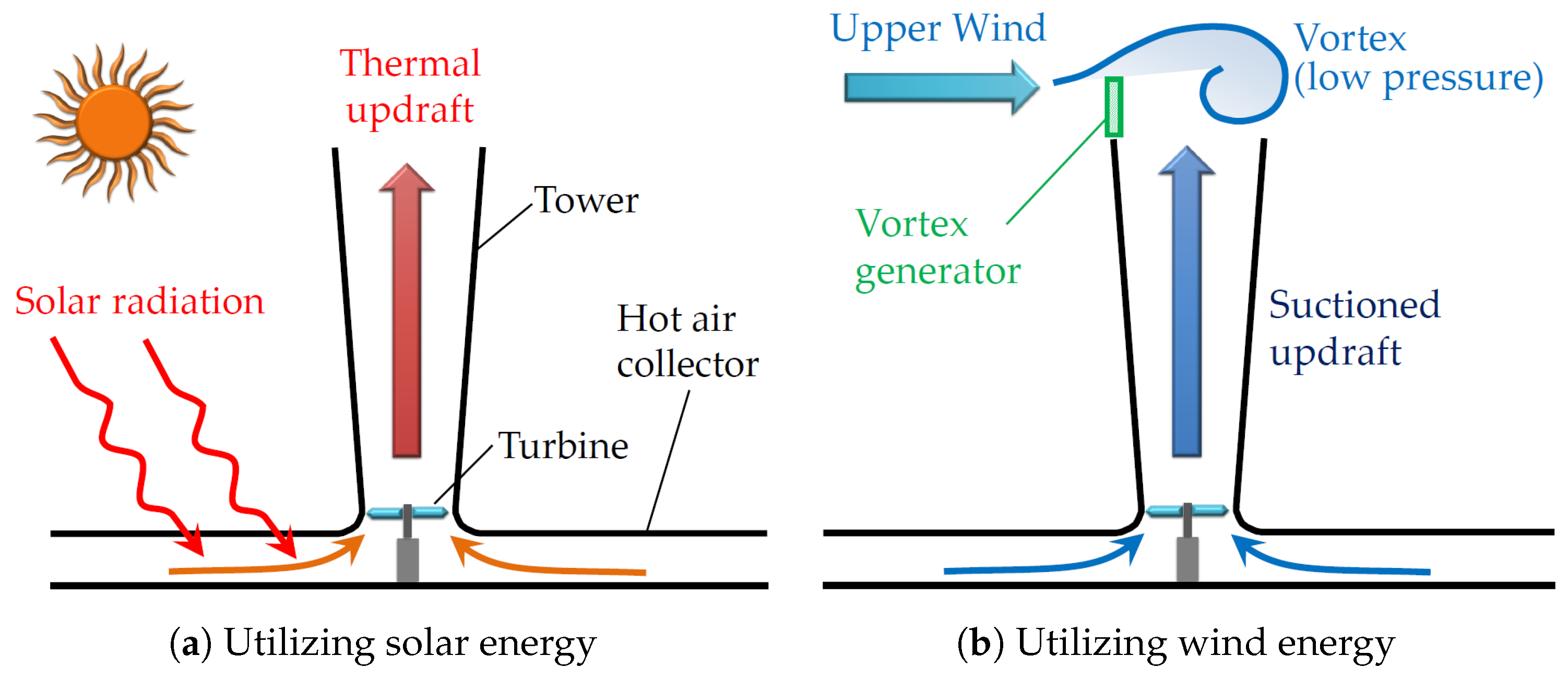
The physical basis of the operation of wind–solar towers (WSTs) is the phenomena of hot air rising to generate airflow streams (greenhouse effect), and the fact that air flows from high to low pressures (buoyancy effect), as shown in Figure 1. The generated airflow streams are of two types, namely thermal updraft and suction updraft. These streams rotate a wind turbine to generate electricity. A WST structure consists mainly of three components: a collector for heating the air, a chimney in the middle of the collector for the heated air to escape, and a wind turbine at the entrance of the chimney to produce electricity through the pressure difference across the turbine.

Solar and wind energy-based hybrid renewable energy systems are relatively new. Solar chimneys which generate power solely from solar energy are outperformed by such systems [22]. Solar chimneys were first designed by Leonardo Da Vinci, who envisioned the chimney tower as a smoke jack 500 years ago [34]. Solar towers, on the other hand, were not proposed for power generation until the nineteenth century. Since then, solar towers have undergone various modifications and improvements [22].

In Manzanares, Spain, the first solar tower prototype has been implemented by a team led by Jörg Schlaich [35,36]. The Manzanares prototype’s main specs were a high chimney of 200 m and a collector diameter of 244 m, and it successfully generated a power of 50 kW. Subsequently, Haaf et al. [37,38] investigated mechanisms for electricity generation using solar chimney power plants (SCPPs). More solar power systems were thus set up in other countries [39] and further studies sought improved power generation methods [40,41]. SCPPs use a large area and have large requirements for construction [42]. They are best suited to countries with vast land, which is cheap and rich in solar flux, like deserts [43,44,45]. However, improvements to the efficiency of SCPP can be achieved by using hybrid systems which utilize more than only thermal updraft for power production, e.g., utilizing wind energy, as in WST systems [33], shown in Figure 1b. Later on, new WST variants were introduced [46,47], with different methods for wind power utilization.

Improvements to the efficiency of WST can also be achieved by tuning the design parameters. Changing the dimensions, configurations, and inclination angles of the collector and/or the chimney can result in a significant improvement in the efficiency. Many analytical, numerical, and experimental studies have been performed for that reason. Innovations for design parameters like divergent tower [48,49,50], sloped collector entrance [51], and chimney-base fillet [52,53] were investigated and reported an efficiency improvement.

Many other parameters can affect the performance of WST, for instance, the heat flux, thermal boundary conditions, heat storage systems, and materials used for the collector roof and for the chimney. Numerical and experimental approaches have been used to study such effects and optimize the overall WST performance [48,54,55,56]. One of the very effective techniques for the prediction of different parameters’ effects on the performance of energy systems is the artificial intelligence technique [57,58].

1.2. Learning Methods

Machine learning (ML) and deep learning (DL) methods represent key artificial intelligence (AI) subfields, and they have gained significant research momentum within the past few years because of their outstanding potential in modeling nonlinear input–output relationships for regression and classification problems. These powerful methods extend to be applied to multivariate problems where the numbers of features or input variables are considerably large. The ML and DL methods proved a huge success in natural language processing (NLP), pattern recognition, computer vision, medical diagnosis, bioinformatics, hurricane assessment [59], as well as the management of the novel coronavirus (COVID-19), and even in student performance prediction [60], and many other applications.

In the renewable energy field, ML/DL have been utilized for many applications, mainly for prediction of the renewable power [61] or the power output of renewable energy systems like wind energy systems [62,63], solar systems [64,65], and other systems, like biomass- and hydrogen-based systems [66]. We should highlight that, recently, there have been several studies utilizing ML/DL for thermal towers only [67,68] or systems that utilize wind only [69]. The studies of hybrid systems using ML/DL [70] are unrelated to WST.

The ML/DL methods are currently available in user-friendly software libraries [71] such as Scikit Learn, TensorFlow, Keras, Pytorch, and CNTK. ML has a wide range of methods/models used for many tasks such as prediction and classification. Among those methods are network-based models like NN and CNN, which are considered as a category of ML called DL.

The ML/DL methods or tasks can be categorized into four categories [72] based on the pattern of learning supervision (whether data are labeled or not). According to these categories, supervised learning is the suitable formulation for our problem/task. As the data are collected from certain sensors, the data are labeled. Also, we need to predict the power output based on certain input feature values, so it is a regression task. The collected dataset is considered tabular data [73].

Notice that NN and CNN are suitable for our physical application with dataset entities collected using sensors as numerical values since the results could be justified with solid mathematical equations. The new boom of large language models (LLMs) [74] will not be suitable in our case since we do not have textual data. Also, LLMs are not preferred with tabular data, as they need high computational power and have many parameters to be tuned. Even with large tabular datasets, there are some suggestions to use some lighter ML models, like gradient boosting [75], instead of DL models like NN and CNN [76].

There have been a few proposed approaches for the modeling of WST systems; however, the performance of such approaches could decline with scale variations [77]. With the collection of adequate data, ML models could have better generalization capabilities, tolerate weather variations, and lead to better modeling and prediction of problems in renewable energy systems. In this paper, the data collected from a wind–solar tower prototype developed and established at Kyushu University [33,78] will be used for predicting the WST power output using a deep learning approach. The authors have previously employed simple ML techniques for WST thermal updraft modeling and prediction [79]. However, predicting the power output for wind-turbine-equipped WST systems is more complicated, and necessitates the use of deep learning methods. Hence, since the WST is considered a new hybrid renewable energy system, there is no data-based power prediction using ML/DL for this system.

1.3. Contribution and Organization

This paper extends our earlier work [79] in which we described in detail the wind–solar tower prototype developed at Kyushu University, and modeled a wind-turbine-free WST system to predict thermal updraft using linear regression. Accurate power prediction could be used for feasibility studies at proposed deployment locations. In our current work, we aim to construct a more elaborate regression model for WST power output prediction when a wind turbine is incorporated into the WST system. With a wind turbine installed, classical ML methods were insufficient for predicting accurate power output. In this work, a deep learning approach is introduced for a more accurate WST power output prediction model. To achieve our goal, we evaluated multiple machine learning models based on quality metrics and selected the best model that balances accuracy and speed. By knowing a set of features like temperature, solar radiation, and wind speed, we could predict the power output using our NN model.

This paper is divided into five main sections. Section 2 describes the data collection process, and provides preliminary data analysis. In Section 3, predictive models and performance evaluation metrics are briefly reviewed. In Section 4, power prediction results are presented for methods of linear regression and nonlinear polynomial regression. In Section 5, we further present detailed results for the deep learning approach. Finally, Section 6 concludes the paper and points out future research directions.

2. Data Collection and Analysis

In this section, we will show the process of data collection and the correlation analysis of all the data for the sake of the feature selection process.

2.1. Experimental Setup and Data Description

Data were gathered using sensors mounted on an established WST prototype for 2 setups:

• WST with no wind turbine: WST system’s output for this setup is the thermal updraft (CH2-7). This case was analyzed in the authors’ previous paper [79].
• WST with a wind turbine: WST system’s output in this setup is the power generated from the wind turbine (CH3-2).

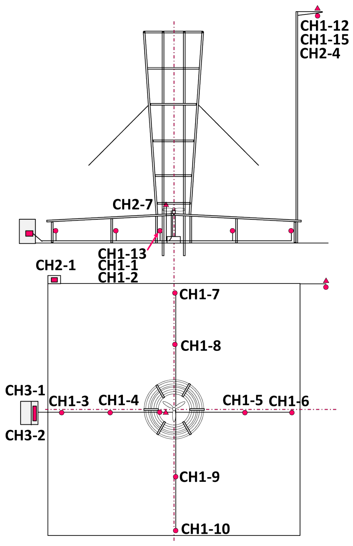
For data collection, the employed sensors are described in [79] and their locations are shown in Figure 2.

Table 1. Channel description and units of the collected WST measurements [79].

Channels	Description	Unit
CH1-1:CH1-10	Temperature (at the base/collector)	°C
CH1-11	Wind speed [Not Used—replaced by CH2-4]	m/s
CH1-12	Temperature of the outside air	°C
CH1-13	Temperature inside the tower	°C
CH1-14	[ - ]	-
CH1-15	Wind direction (outside the tower)	°
CH1-16	Wind turbine speed [Not Used—replaced by CH3-1]	rpm
CH2-1	Solar radiation (by a pyranometer)	kW/m2
CH2-2	Electricity generation capacity (inside the collector)	kW
CH2-3	Electricity generation capacity (outside the collector)	kW
CH2-4	Wind speed of the outside air, u	m/s
CH2-5	Wind turbine output [Not Used—replaced by CH3-2]	kW
CH2-6	Wind turbine rotation speed [Not Used—replaced by CH3-1]	rpm
CH2-7	Internal ascending wind speed, w (at the rotor)	m/s
CH2-8	Wind direction (at the rotor)	°
CH3-1	Wind turbine speed	rpm
CH3-2	Wind turbine power output	mW
CH3-3	Voltage after rectification	V

summarizes the data types collected from all channels and

Table 2. Statistical data of the collected dataset.

	Mean	Std	Median	Min	Max
CH1-1	15.883930	10.182027	17.005128	−4.886447	46.015385
CH1-2	22.838014	11.073108	23.926740	1.476190	55.380220
CH1-3	−23.146420	40.460299	−58.956777	−59.947253	49.633824
CH1-4	9.604102	28.064369	18.502514	−59.873260	57.870330
CH1-5	23.455295	12.954458	23.926007	−0.119414	65.056410
CH1-6	22.208231	13.394067	22.536785	−1.655678	64.850549
CH1-7	21.797247	11.382459	22.837363	0.054212	58.169963
CH1-8	23.435457	12.596312	23.887179	0.715018	65.205861
CH1-9	23.764470	12.989383	24.152381	0.258521	61.990476
CH1-10	24.392065	11.179543	24.721612	1.219048	55.293187
CH1-11	0.770427	0.843193	0.493407	0.371913	12.127253
CH1-12	18.590188	9.094985	19.993407	−0.939927	42.008059
CH1-13	21.766755	10.837656	22.880957	1.054350	53.625416
CH1-14	0.006526	0.002010	0.006418	0.000974	0.016168
CH1-15	162.373576	80.910417	165.445252	1.146113	358.577127
CH1-16	35.300166	50.193472	21.460317	−12.000000	546.046398
CH2-1	0.158096	0.266467	0.005613	−0.037444	1.510260
CH2-2	0.000317	0.000454	0.000122	0.000000	0.003373
CH2-3	0.002149	0.001351	0.002015	0.000020	0.008262
CH2-4	1.452632	1.196944	1.154133	0.255487	12.407637
CH2-5	0.259529	0.222899	0.225967	0.032336	1.948046
CH2-6	0.033535	0.063375	0.008568	0.000000	0.652137
CH2-7	1.295922	0.681615	1.274382	−0.086350	5.324969
CH2-8	52.918118	49.960923	31.695513	4.703755	4177.547495
CH3-1	49.347027	77.631788	0.000000	0.000000	343.550833
CH3-2	980.748950	2093.888824	2.266667	0.000000	30,242.133333
CH3-3	4.375860	6.432452	0.252700	0.034283	24.647483

shows the basic statistical values of the collected dataset of 358,751 samples. In this paper, we will focus on the WST configuration equipped with a wind turbine. This wind turbine has a rotor diameter of 1380 mm, like the wind lens turbine [80]. The wind blade is of the MEL type developed at the National Institute of Advanced Industrial Science and Technology (AIST) [81]. The blade was designed in Furukawa’s Laboratory of the Department of Mechanical Engineering at Kyushu University [82]. The data were collected over a 10-month period, leading to 358,751 samples after averaging and data cleaning.

2.2. Correlation Analysis

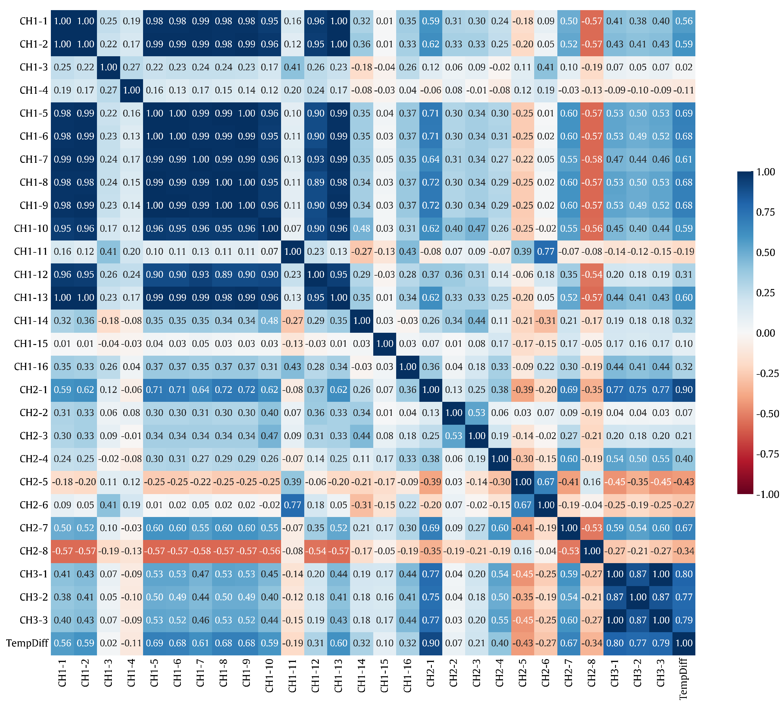
We investigated the pairwise correlation for all pairs of WST input features according to the Pearson correlation coefficient (PCC), and the best uncorrelated features were selected based on that. The correlation results are visualized as a heatmap as shown in Figure 3. As a subset of this, the correlation of the WST output power with each WST input feature is computed as a sensitivity measure of the power output with respect to the input features. For all WST input–output pairs, the absolute PCC values are shown in Figure 4.

According to Figure 4, all correlation values are fairly significant. So, no features can be confidently discarded. Instead, all features shall be examined in the subsequent regression analysis. However, the features of solar radiation [CH2-1] and wind turbine speed [CH3-1] are probably the most important ones based on their high correlation with the output power. For the regression model, the output is the power output [CH3-2] which will be modeled/predicted, and the inputs are all other features stated in Figure 4.

3. Predictive Models

In this section, we will show how the regression models are assessed and how to avoid the overfitting problem. Then we will give a quick overview of the deep learning technique.

3.1. Performance Assessment

For constructing and evaluating predictive models of the WST output power, the collected experimental data samples were split into training, testing, and validation sets. The training set was assigned 70% of the samples for model training. The test set had 20% of the samples for model testing based on specified quality metrics. About 10% of the data was allocated to the validation set whose elements have never been used in model training. The validation samples will be used to evaluate the generalization performance of the trained model. The validation set could be chosen based on certain criteria. In our work, the validation set contains exactly the largest amount of measurements collected in the first day of experiments.

For output power prediction, multiple models were trained. The derived models were largely complex and difficult to grasp, except for the linear regression model. The model performance is evaluated for the testing data by comparing the model prediction to the ground-truth power output measurements.

During the training of the model, quality metrics were utilized as cost functions that needed to be minimized. The cost functions can be minimized by different optimization algorithms such as the gradient descent one. For the test data, the quality metrics were used for performance evaluation. The quality metrics used in this work are explained in detail in the authors’ previous paper [79]. In the machine learning topic, the quality metrics are considered the performance measure that judges the accuracy/capabilities of the model. Usually, the coefficient of determination ($R^2\in [0,1]$) is used, as it shows a normalized accuracy representation.

3.2. Model Representation

In this work, we will choose the mean-square error as the performance measure or the cost function from the set of quality metrics. Our goal is to identify the feature weight values that minimize the mean-square error. The following is a mathematical representation of the minimization problem [83]:

$$\underset{\theta }{\mathrm{minimize}}\underset{\mathrm{cost} \mathrm{function} J\left(\theta \right)}{\underbrace{{\displaystyle \frac{1}{2m}}\sum _{i=1}^m{(\stackrel{\stackrel{\mathrm{Predicted} \mathrm{value}}{︷}}{h_{\theta }\left({\mathbf{x}}^{\left(i\right)}\right)}-\stackrel{\stackrel{\mathrm{True} \mathrm{value}}{︷}}{y^{\left(i\right)}})}^2}}$$

(1)

To numerically solve this minimization problem, a gradient descent algorithm will be used [84] with the following update rule:

$$\mathrm{repeat}\mathrm{until}\mathrm{convergence}\{{\theta }_j:={\theta }_j-\alpha \underset{\mathrm{Derivative}\mathrm{term}}{\underbrace{{\displaystyle \frac{\partial }{\partial \theta }}J\left({\theta }_{\mathit{j}}\right)}}\}$$

(2)

where $\alpha$ is the learning rate which represents the steps. ${\theta }_j$ is the j-th feature and j is from 0 to the number of features m. The symbol $:=$ denotes an iterative update process, which has two cases:

• Derivative term has a negative sign: ${\theta }_j$ will decrease approaching the local minimum point.
• Derivative term has a positive sign: ${\theta }_j$ will increase approaching the local minimum point.

We do not need to worry about getting stuck in local minima because the cost function is convex and has one global minimum point.

3.3. Over-Fitting Problem

Over-fitting is a common explanation for the poor generalization performance (expressed by high generalization error) of a predictive model on new test data.

When the available data are divided into three sets, the number of samples used for model training is reduced. As a result, the results can depend on the random selection pattern of the training and validation samples. This dependence can be reduced through a cross-validation (CV) scheme. In this scheme, a test set is held out for final evaluation, but a validation set is no longer needed. Specifically, for the k-fold CV scheme, the training set is equally split into k subsets. Each of the k folds undergoes the following procedure:

• The model is trained based on (k − 1) data folds.
• The trained model is tested according to the remaining data fold. This fold being treated is used as a test set to compute the mode’s performance according to quality metrics.

The output performance measure of the k-fold cross-validation scheme is the average of all values computed through the loop. While this scheme has a high computational cost, it effectively exploits datasets with small numbers of samples.

3.4. Deep Learning Overview

In this subsection, a quick overview of the NN representation and the tuning strategy for the NN architecture is given.

3.4.1. NN Representation

Artificial neural network (ANN) models have been gaining increasing research focus because of their remarkable potential in modeling nonlinear input–output relations. Generally, the artificial neural networks mimic the behavior of the biological neural networks of the human brain. A “neuron” in an ANN is a biological-neuron-like mathematical function that collects and classifies information according to some predetermined architecture. Recently, in the DL era, it has become more common to shorten ANN to NN and still refer to the mathematical neural network, not the biological one.

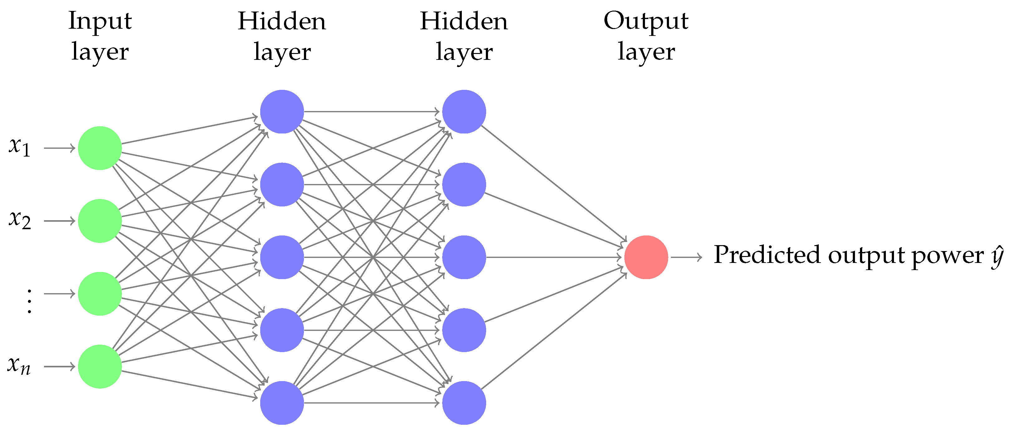
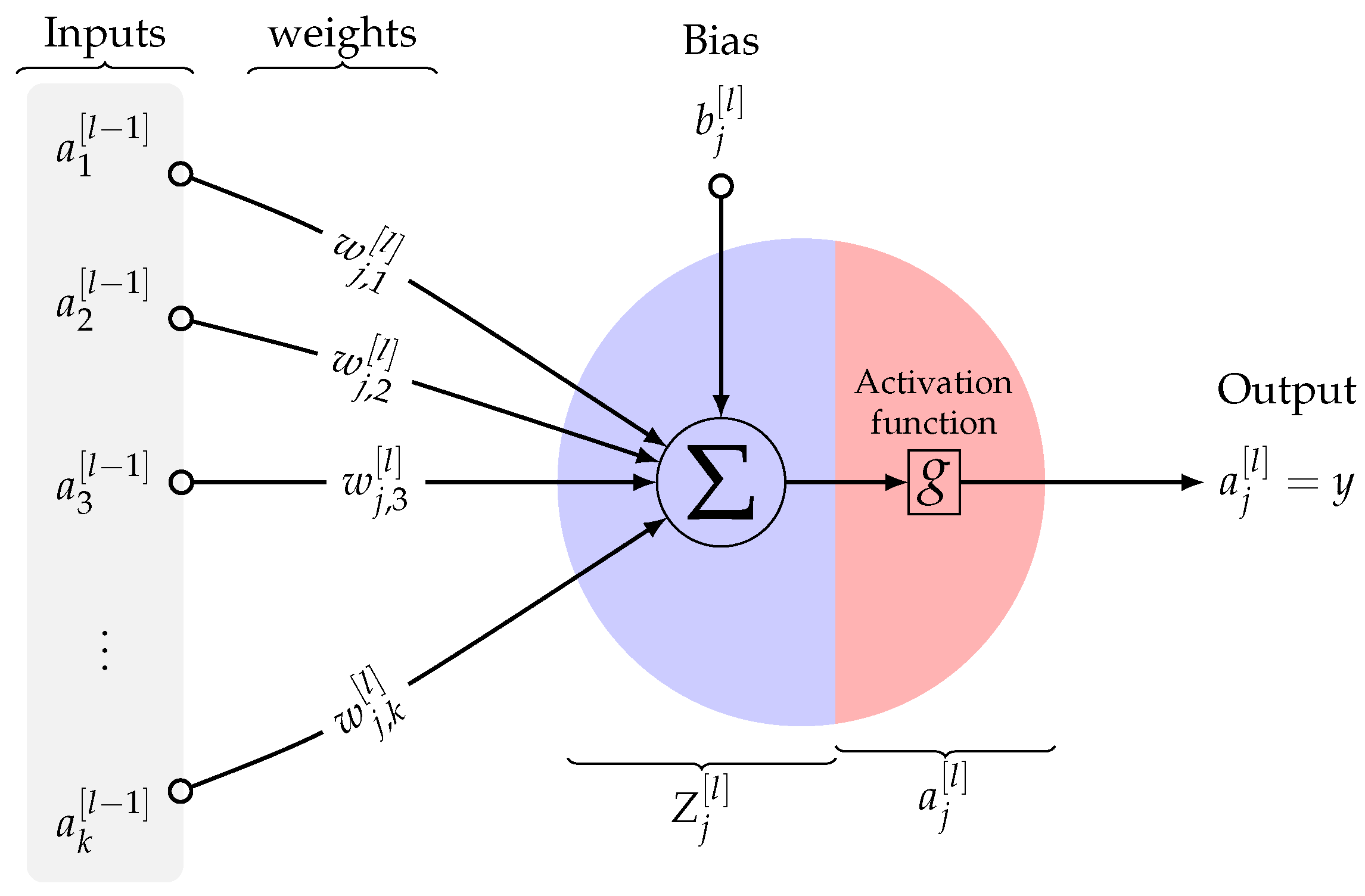
NN is essentially composed of layers of interconnected nodes. Figure 5 shows the adopted NN model (with two hidden layers) for WST power output prediction. Each node in the network model is a perceptron that is basically used to perform multiple linear regression. The perceptron feeds the input signals into an activation function. The activation function will determine the output of the learning model, its accuracy, and also its computational efficiency. An activation function can be made linear or nonlinear according to the complexity of the prediction. Figure 6 shows a schematic representation of a single perceptron that involves linear summation and nonlinear activation operations.

As mentioned above, in a neural network or multi-layered perceptron (MLP), perceptrons/neurons are arranged in interconnected layers. The input network layer collects input patterns, while the output layer returns predicted classification or regression outputs. In our work, the adopted network is used to predict the WST power output. The weights and biases within the hidden layers are fine-tuned, and the margin of error of the network is minimized. The hidden layers essentially extrapolate the salient features of the input data that have high potential for predicting the WST output power.

3.4.2. Hyper-Parameter Tuning

A neural network has many parameters to be tuned. In this subsection, we will present the tuning strategy that we followed.

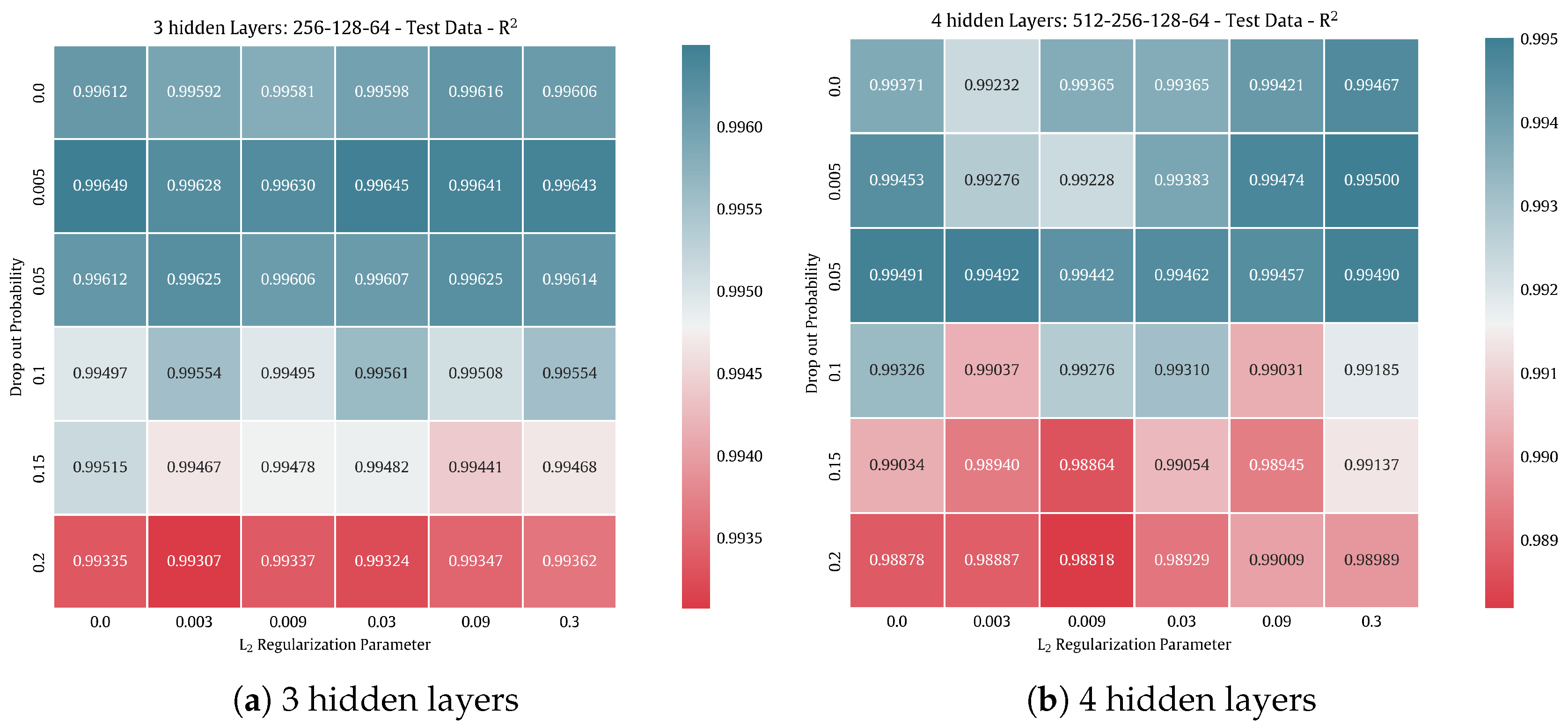
• # hidden layers: We usually chose three to five for the scale of our problem. We tried three, four, and five hidden layers. Increasing the number of layers could increase the accuracy slightly but with a huge increase in training and evaluation time. Sometimes, the complexity that comes from increasing the number of layers could lead to a small reduction in accuracy, as it will be shown later in Figure 15.
• # neurons in each hidden layer: We follow the strategy of choosing powers of 2 in a descending way while going deeper within the hidden layers [85] (for four hidden layers: 512-256-128-64).
• # input neurons: One per input feature.
• # output neuron: One per prediction dimension.
• Hidden activation functions: We used exponential linear unit (ElU). However, there are many other activation functions that could be used based on the type of prediction task [86].
• Output layer activation functions: Could be linear, RelU (for positive outputs), and Tanh (bounded outputs).
• Optimizer: We chose “Adam”, as it combines the RMSprop and momentum techniques.
• Learning rate: It could affect the performance dramatically. Choosing smaller values will lead to better accuracy, but with higher computational cost. We used a value of 0.001.
• Batch size: Like learning rate, smaller values will lead to better accuracy, but with higher computational cost. However, it is better not to use a batch size less than 32.
• # epoch: We used a high number then used a callback to scan the whole domain and return the epoch that leads to the best accuracy. However, this is used only when we have enough computational power and time. If we lack these two factors, we could use early stopping techniques, which stop once the error starts to increase.
• Drop-out and Regularization: Used to solve the overfitting problem. These two parameters will be tuned by trial, as it will be shown later in Figure 15.

Notice that no normalization is needed before feeding the data to the NN [72].

3.4.3. CNN Representation

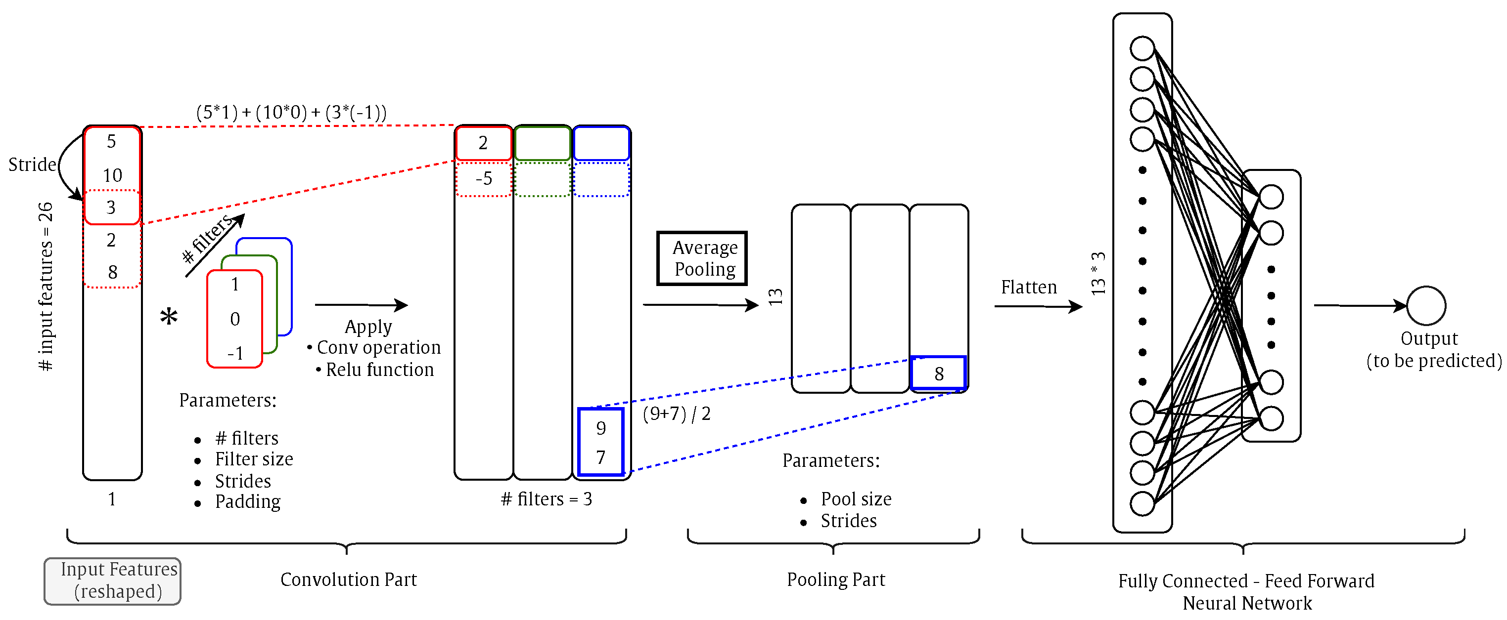
Convolutional neural networks (CNNs or ConvNets) are a class of artificial neural networks which are widely used in image processing applications for classification tasks. However, it could be used for regression tasks, such as 1-D ConvNet. CNN has superior performance with image, speech, or audio signal inputs. The ConvNets are constructed of a Conv part, a pooling part, and a fully connected feed-forward NN. The Conv part is the core building block of a ConvNet and it has three hyper-parameters:

• Number of filters: Affects the depth of the output.
• Stride: The distance that the filter/kernel moves over the input matrix.
• Zero-Padding: Used when the filters do not fit the input matrix.

Following each convolution operation, a ReLU transformation is applied introducing non-linearity to the model. Then, there is a pooling part to reduce the volume size. In the end, the volume is flattened and will be an input for a feed-forward NN, as shown in Figure 7.

4. ML Results

This section represents the results of different ML algorithms for WST power prediction and we compare these algorithms according to several quality metrics as well as the training and evaluation times, as shown in

Table 3. Power prediction quality metrics (performance measure) for multiple models. Red boxes highlight the models that we will focus on.

Model	MSE	${\mathit{R}}^2$	Max Error	Exp. Var.	MAE	Train Time	Evaluation Time
Neural Networks	19,857.778221	0.995460	5685.913585	0.995462	51.245220	5632.759634	2.616292 × 10−5
Decision Tree Regressor	33,498.168299	0.992341	5836.616667	0.992342	56.810956	8.828785	1.371223 × 10−7
Gradient Boosting	34,502.391054	0.992112	7462.057059	0.992112	61.865121	219.236386	9.038692 × 10−7
Non-linear Regression	34,526.695194	0.992106	6904.443909	0.992106	88.490677	4.647073	6.831196 × 10−6
linear Regression	717,393.478707	0.835984	16,571.690531	0.835984	506.781286	0.392245	3.883074 × 10−7
Ridge Regression	720,205.905602	0.835341	16,545.019265	0.835341	507.364975	0.400614	1.285000 × 10−7
Lasso Regression	729,781.443313	0.833152	16,995.194940	0.833152	506.802259	28.659264	1.387964 × 10−7
Adaptive Boosting	792,388.384346	0.818838	7101.254203	0.956526	785.552367	63.345530	4.403798 × 10−6
Elastic Net Regression	860,393.191587	0.803290	21,024.517318	0.803290	526.140660	28.262666	1.390596 × 10−7
SVM Regressor	1,022,548.0001	0.766216	22,071.330	0.766919	436.70750	100.11386	7.860384 × 10−8

. The best model is thus presented in detail. Standard Scikit learn implementations were used for all machine learning algorithms [87]. Detailed descriptions of the quality metrics can be found in [79].

The results in Table 3 show that power prediction performance based on linear regression is not accurately sufficient (contrary to its good performance in predicting the thermal updraft [79]). The non-linear polynomial regression shows acceptable performance outcomes. Gradient boosting is an ensemble model which depends mainly on the used models and needs intensive hyper-parameter tuning. The decision tree model has a lot of hyper-parameters to be tuned and has a tendency to overfit. The neural networks seem to be the most promising models. Table 3 is considered a quick guide to help decide which model will be suitable for our dataset.

To understand how powerful the neural network is, we evaluate $\sqrt{\mathrm{MSE}}=140.92$, which represents the error value within the power output range. Knowing that the power output varies from 0 to 30,242.1333, this means the error percentage is 0.466%. Later, we will present more deep learning results based on Keras/TensorFlow 2.16.2 libraries, which gives us more control over the hyper-parameter tuning process, resulting in a more accurate model.

Other parameters to be considered while choosing a suitable model are the training time and evaluation time. The training time is the time that the model takes to be trained. After the model is trained, new input data could be used to predict the output; the required time for the process of one sample is the evaluation time. In practice, it is possible to take time building the model, but in real applications, the evaluation time is crucial.

We will show the linear regression model and visualize its results in the two following subsections. Its performance is thus enhanced through hyper-parameter tuning. Afterwards, the results of the non-linear polynomial regression model shall be explored.

4.1. Linear Regression Model

Here, the linear regression (LR) model results of WST power prediction will be presented. The LR model is represented mathematically as follows:

$$\widehat{y}=h_{\mathit{\theta }}\left(\mathit{x}\right)={\mathit{\theta }}^{\mathit{T}}·\mathit{x}=\begin{array}{c}\left[\begin{array}{cccc}{\theta }_0& {\theta }_1& \cdots & {\theta }_n\end{array}\right]\end{array}\left[\begin{array}{c}{x}_0\\ x_1\\ ⋮\\ x_n\end{array}\right]$$

(3)

where $\mathit{\theta }$ is a column vector of model parameters, including the bias term ${\theta }_0$ and the feature weights ${\theta }_1$ to ${\theta }_n$, where n is the number of features (n = 26 in our work). Also, $\mathit{x}$ is a column vector of the features $x_0$ to $x_n$, with $x_0$ always equal to 1. Finally, $h_{\theta }$ is the prediction or hypothesis function, and $\widehat{y}$ is the predicted value.

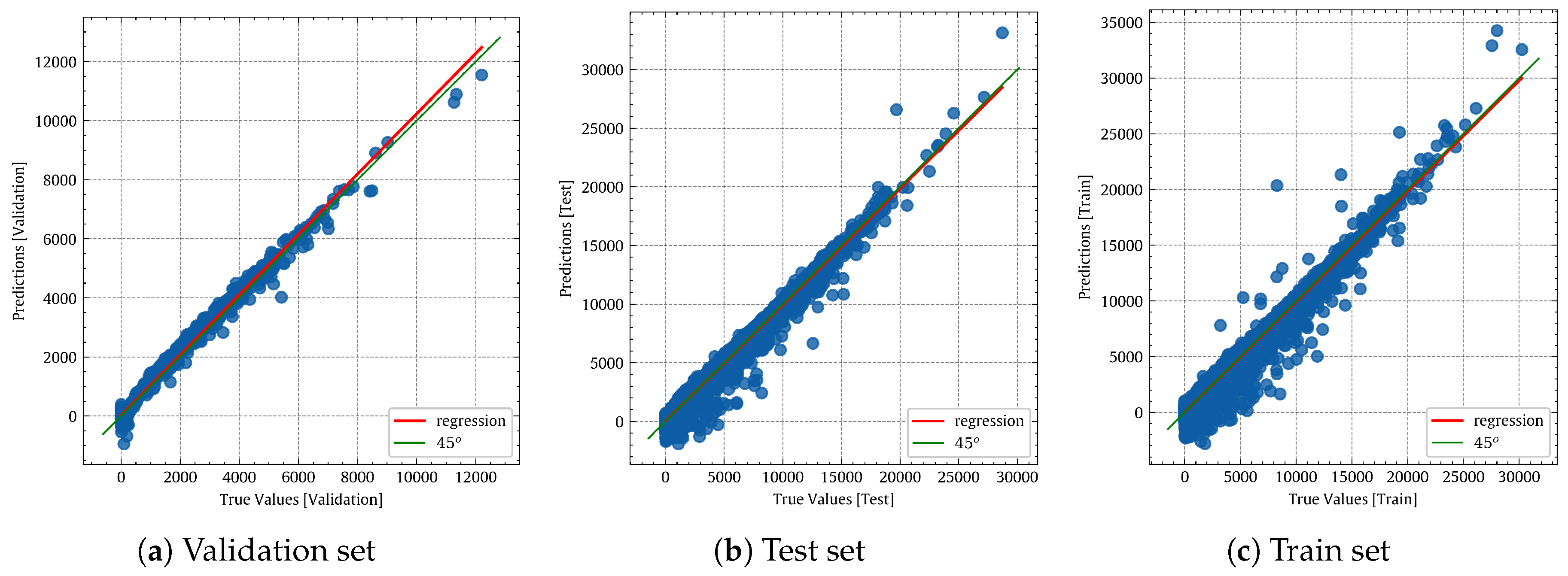
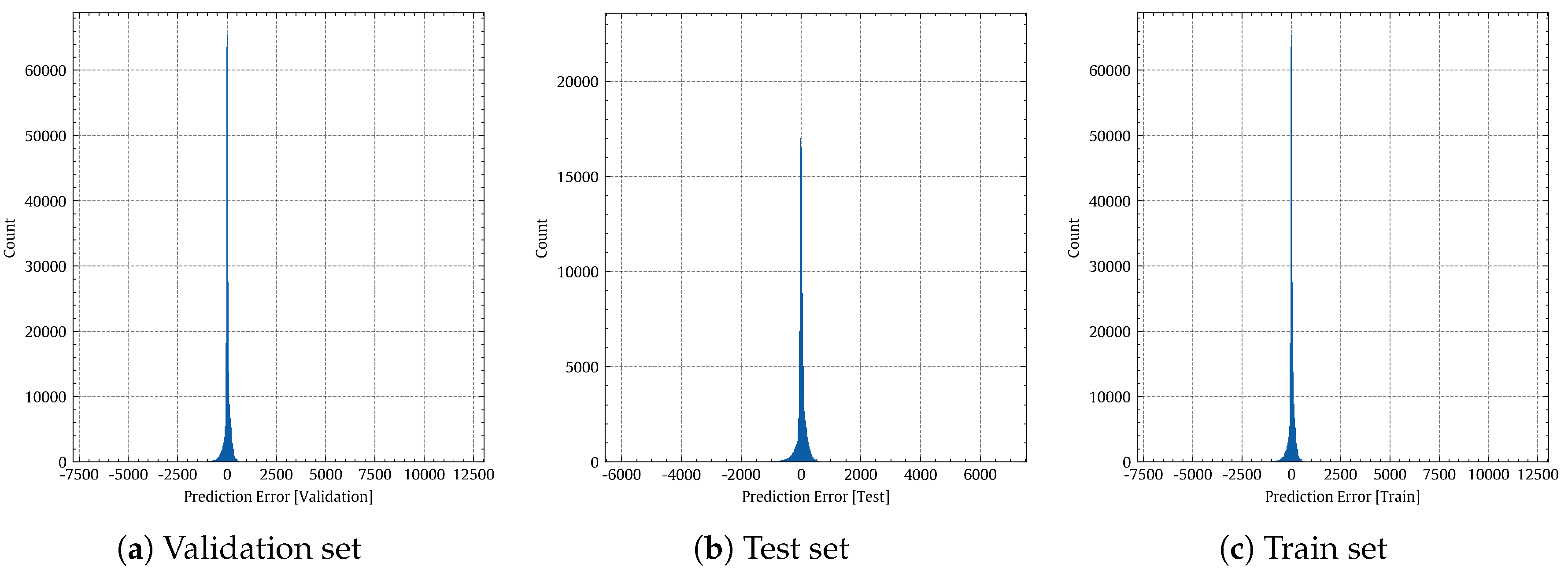
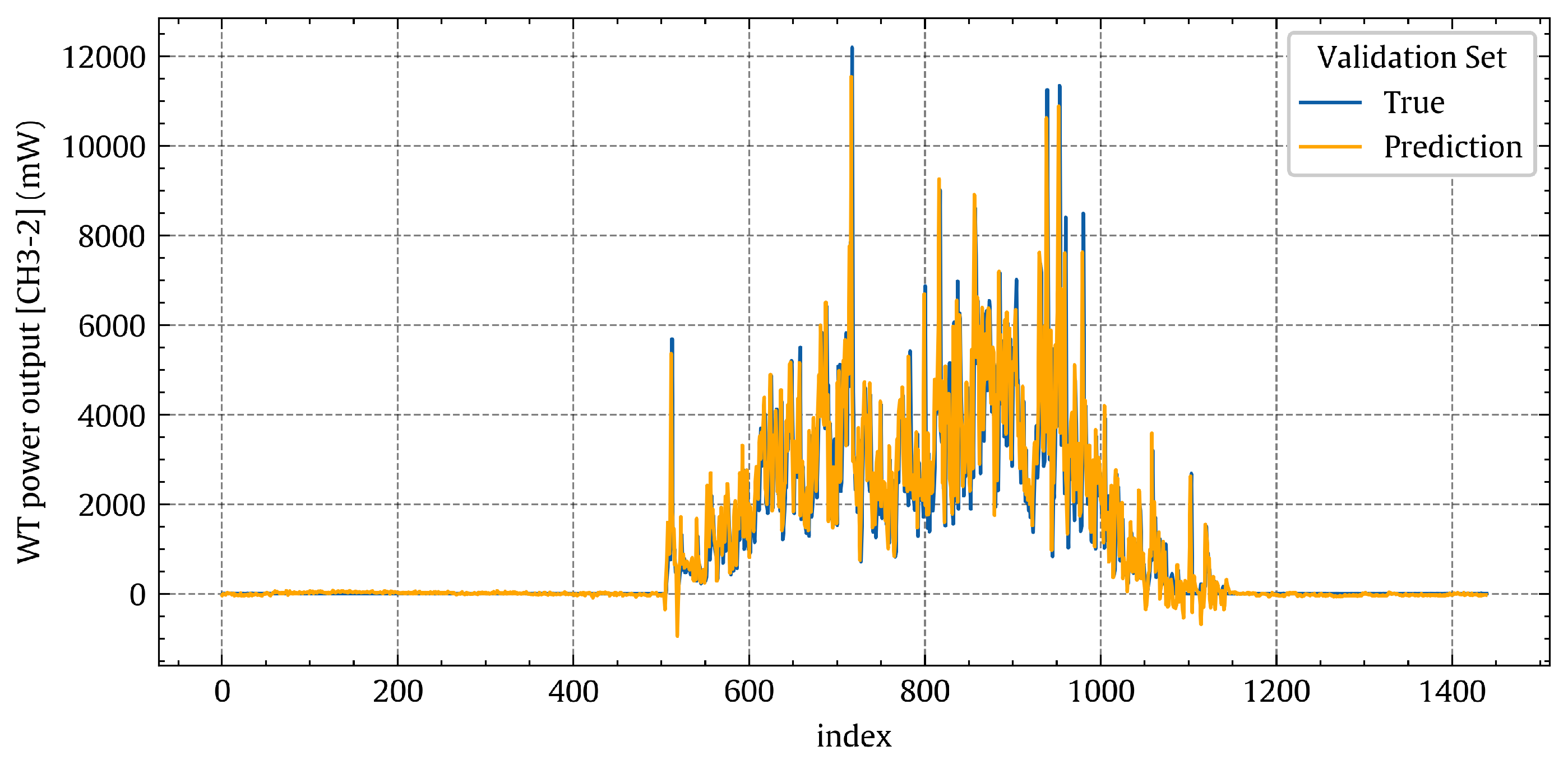
Figure 8 indicates the accuracy level of the linear regression model. The green line with the $45°$ slope represents a perfect model. The LR model (in red) clearly deviates from the perfect model (in green). The prediction error is very high, as shown in Figure 9. In Figure 10, the temporal patterns of the true and predicted power values are shown with the blue and orange lines, respectively, for the LR model on the validation set. The two lines representing the true and predicted values do not fully overlap.

4.2. Tuning Ridge Model

In this subsection, we seek to enhance the performance of the linear regression model by tuning its hyper-parameters. For this, we will use the ridge regression model, built in sci-kit learn [87], which is a variant of the linear regression model with more hyper-parameters. The best hyper-parameter values are found through a random search approach followed by a grid search within reduced search regions [88]. The best hyper-parameter settings were found to be ’alpha’ of 0.1 with normalization, no fit intercept, and a Cholesky solver. 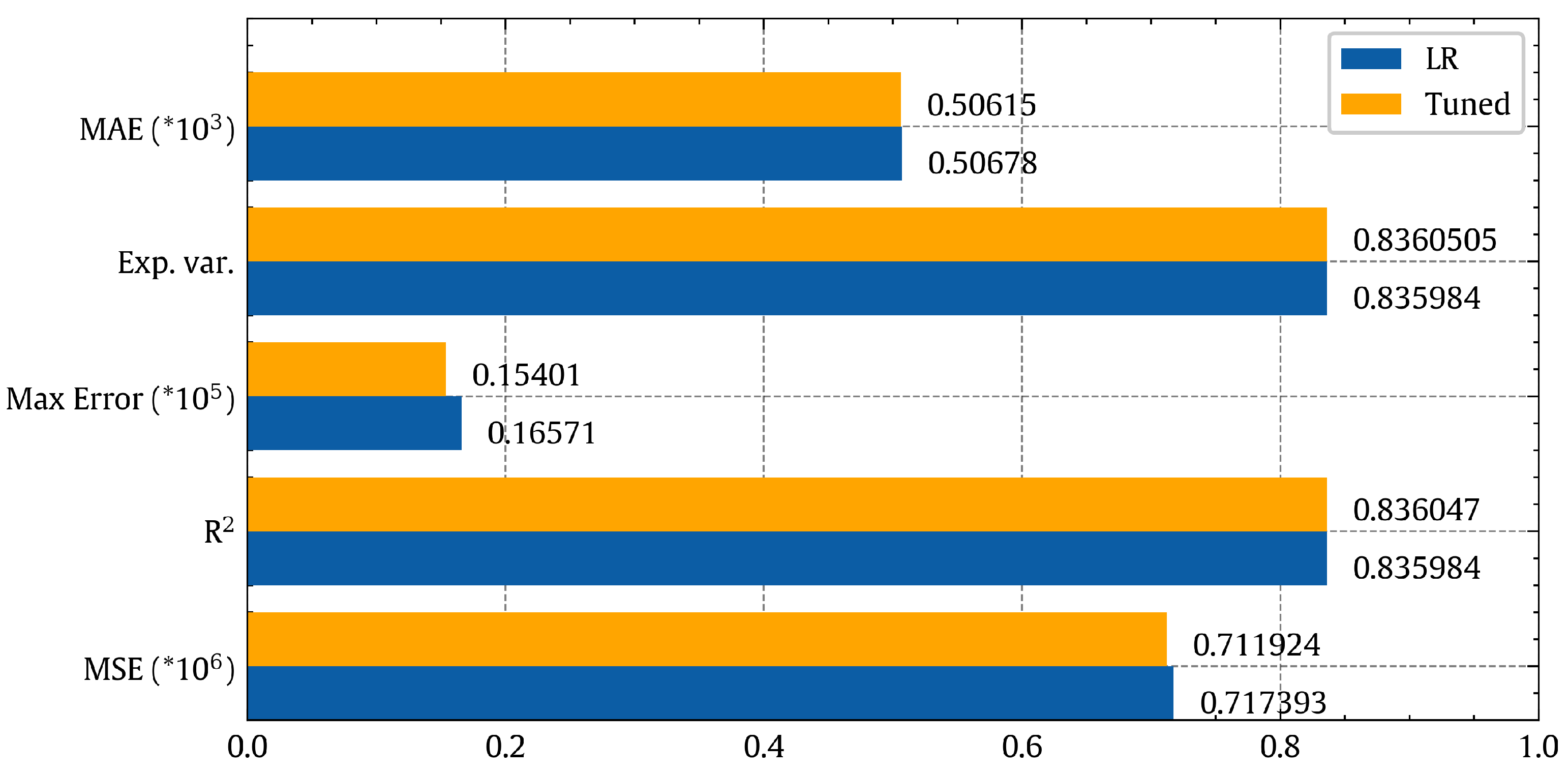Figure 11 shows that this fine-tuning resulted in little enhancement where the accuracy is still largely the same. So, we explored a non-linear regression modeling approach to try to achieve better power prediction performance.

Figure 11 shows that the enhancement due to tuning is not huge and the accuracy still not acceptable. So, we have to go for non-linear regression.

4.3. Non-Linear Regression Model

In this subsection, we present the WST power prediction results for a simple second-order polynomial regression model. This model can be represented mathematically as:

$$\widehat{y}=h_{\mathit{\theta }}\left(\mathit{x}\right)={\mathit{\theta }}_{\mathbf{0}}+{\mathit{\theta }}_{\mathbf{1}}^{\mathbf{T}}·\mathit{x}+{\mathit{\theta }}_{\mathbf{2}}^{\mathbf{T}}·{\mathit{x}}^2$$

(4)

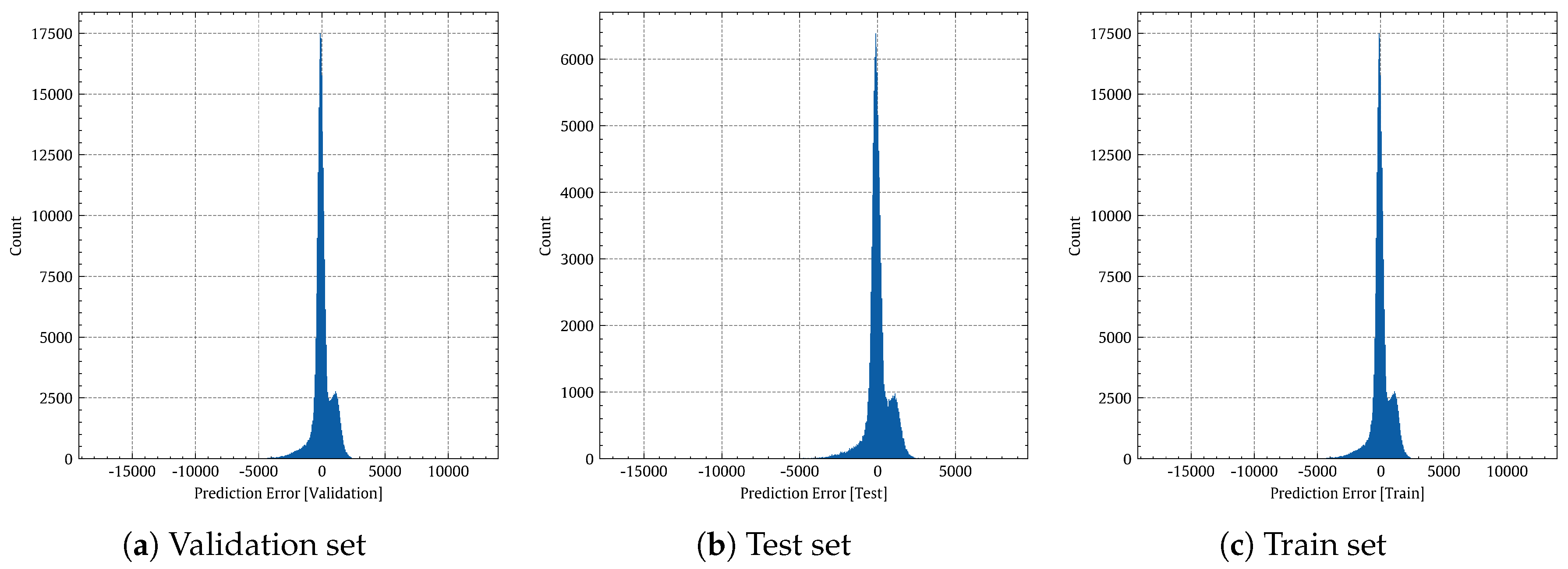
Figure 12 shows that the curve of the non-linear polynomial model (red) closely matches that of the perfect model (green). A visual comparison of Figure 8 and Figure 12 shows that the non-linear polynomial model is superior to the linear regression one. Figure 13 shows histograms of the prediction errors made by the non-linear regression model on the validation, test, and training sets, respectively. 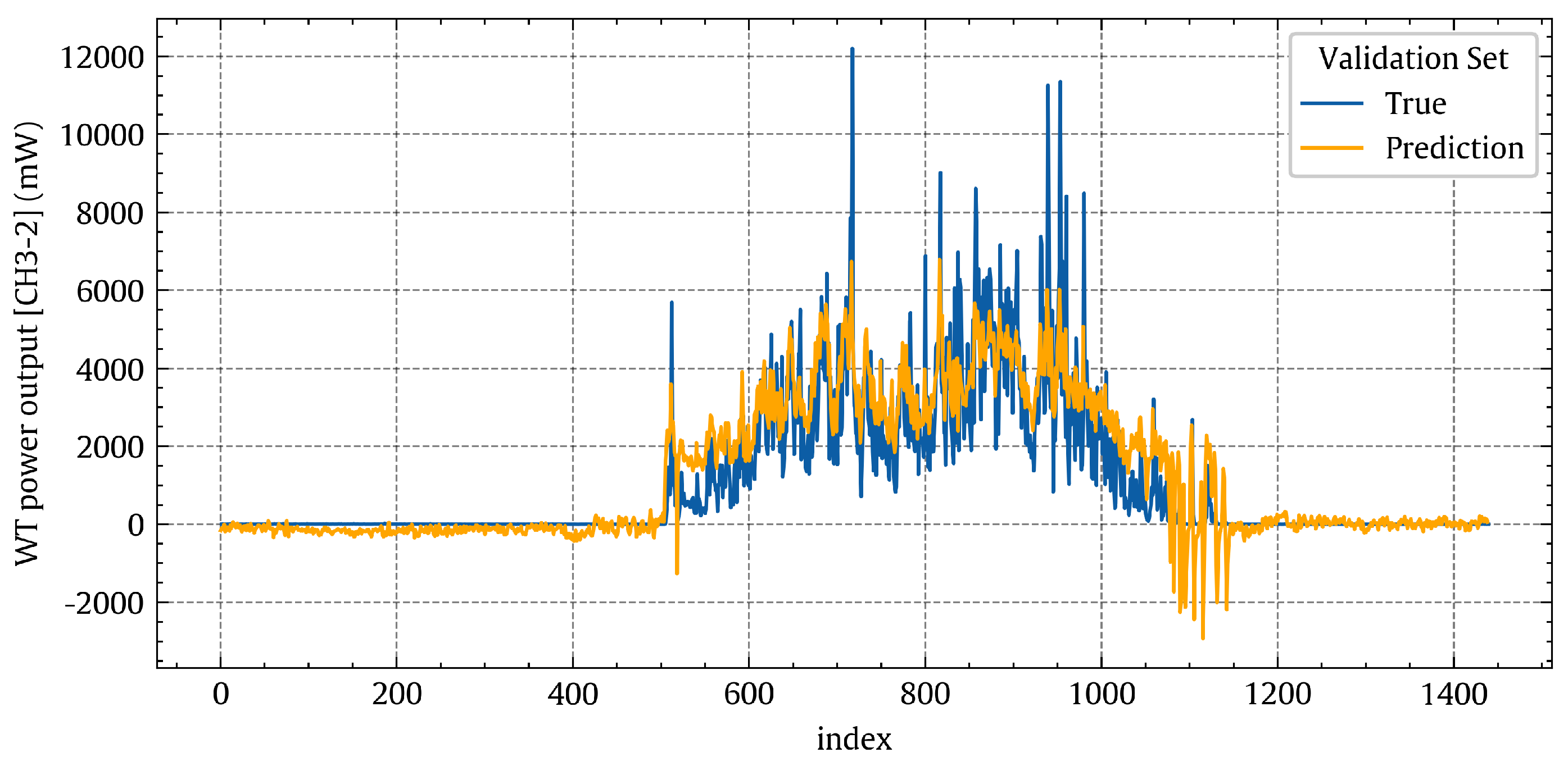Figure 14 shows the temporal variations of the true power output values (blue line) and the associated predicted values (orange line) for the non-linear regression model on the validation set. Indeed, a good agreement can be observed between the true values (blue line) and the predicted values (orange line).

5. DL Results

In this section, we will present the deep learning results, using feed-forward NN and convolutional neural network, in the following two subsections.

5.1. NN Results

For neural network implementation, we created a regression-based deep neural network with exponential linear unit (ElU) activation functions [86] using TensorFlow and Keras [89] libraries. We experimented with three hidden layers of 256, 128, and 64 neurons, respectively. Also, we used an Adam optimizer [90] for over 500 iterations, and we used callback to return the best number of epochs instead of using an early-stopping criterion [91]. For regularization [92], we used a dropout technique to avoid overfitting [93].

Table 4. Keras model summary for a network of 3 hidden layers.

Layer (Type)	Output Shape	No. Param
dense-1 (Dense)	(None, 256)	6912
dropout-1 (Dropout)	(None, 256)	0
dense-2 (Dense)	(None, 128)	32,896
dropout-2 (Dropout)	(None, 128)	0
dense-3 (Dense)	(None, 64)	8256
dropout-3 (Dropout)	(None, 64)	0
dense-out (Dense)	(None, 1)	65
Total params: 48,129
Trainable params: 48,129
Non-trainable params: 0

shows a summary of the deep learning architectural features including the dimensions of the dense layers, the number of trainable parameters in each layer, and the total number of trainable parameters. Note that there is no transfer learning method that has been used which makes the non-trainable params equal to zero. Also, the batch size is variable, which makes the output shape include “None”.

Following the tuning strategy presented in Section 3.4.2, we performed 36 trials, according to the dropout and regularization parameters, per each three- and four-hidden-layer architectures, as shown in Figure 15.

Then, the best-tuned model is selected. According to Figure 15, using three hidden layers with dropout = 0.5% and no L₂ regularization leads to R² = 0.99734.

Figure 16 highlights the evolution of the training and test losses with training epochs. After the model has been trained to an acceptable error threshold, it can be utilized to forecast WST output power values for unfamiliar/new input features. It could be noticed that the error dropped dramatically within the first hundred epochs then become steady.

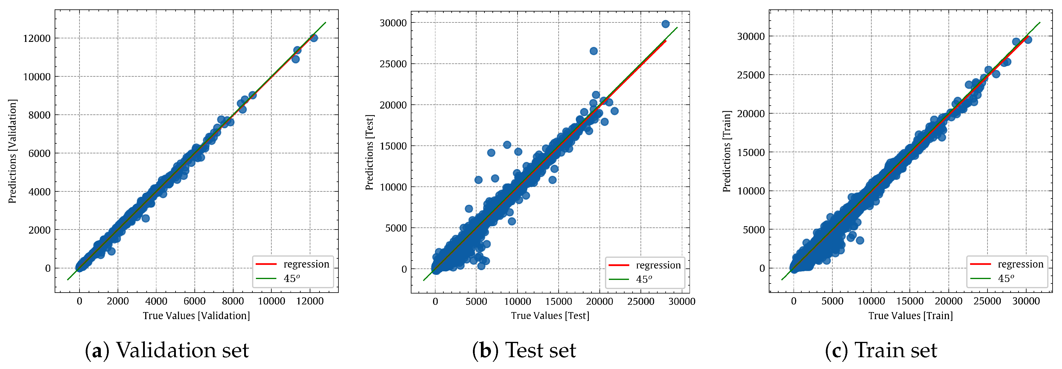
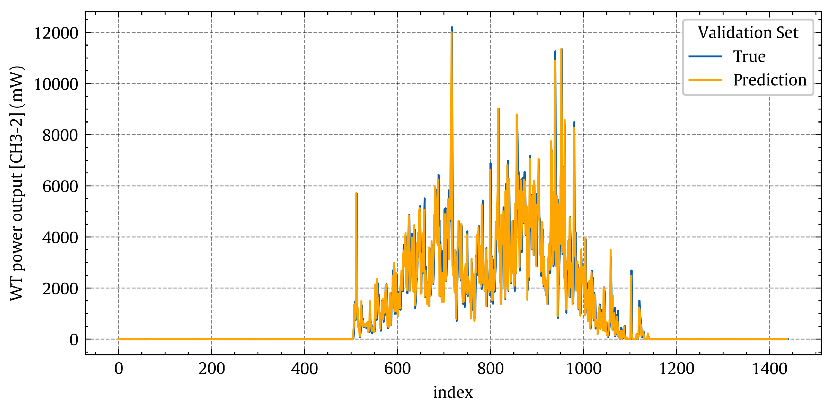
Figure 17 shows the true values vs. predicted values of the NN model. If we visually compare Figure 12a and Figure 17a, it is obvious that the neural network is better than the non-linear regression, as the red and green lines are almost identical. Figure 18 shows the true and predicted values of the validation set. By comparing Figure 14 and Figure 18, the superiority of NN over non-linear regression could be noticed, especially at the high power output values.

5.2. CNN Results

For network implementation, we created a regression-based 1-D convolutional neural network with four convolutional layers using TensorFlow and Keras [89] libraries. These layers are constructed of two parts: conv part and pooling part. The conv part consists of filter size = 3, Padding = “same” to make the output size of each conv part equal to the input size, and strides = 2. Also, the number of filters was chosen in an ascending way (8-16-32-64). Each conv part was followed by an “average pooling” part with pool size = 2. The output of the four convolutional layers was passed to a fully connected feed-forward neural network of two layers with 64-32 neurons and ELU activation function. The Adam optimizer with learning rate = 0.001 was used for the learning process.

Even though CNN has high prediction capabilities, it did not enhance the accuracy, as shown in Figure 19. Also, it needs more computational cost, as the training time and evaluation time are almost doubled compared to NN results of the previous subsection. Consequently, we will stick with the NN model with three hidden layers.

There are other methods used with tabular data, such as TabNet [94]. It is designed for tabular data with a large number of features, as it uses sequential attention to choose which features to reason from at each decision step. The results showed that it is not suitable for our dataset with 26 features only.

Table 5. Summary of the results.

Model	Tool	R2	MSE	MEA
LR	Scikit Learn 1.2.2	0.835984	717,393.4	506.78
TabNet	PyTorch 2.3.1	0.0.98485	66,567.3	93.04
NLR	Scikit Learn	0.992106	34,526.6	88.49
NN	Scikit Learn	0.995460	19,857.7	51.24
CNN	TensorFlow	0.99647	15,450.28	45.87
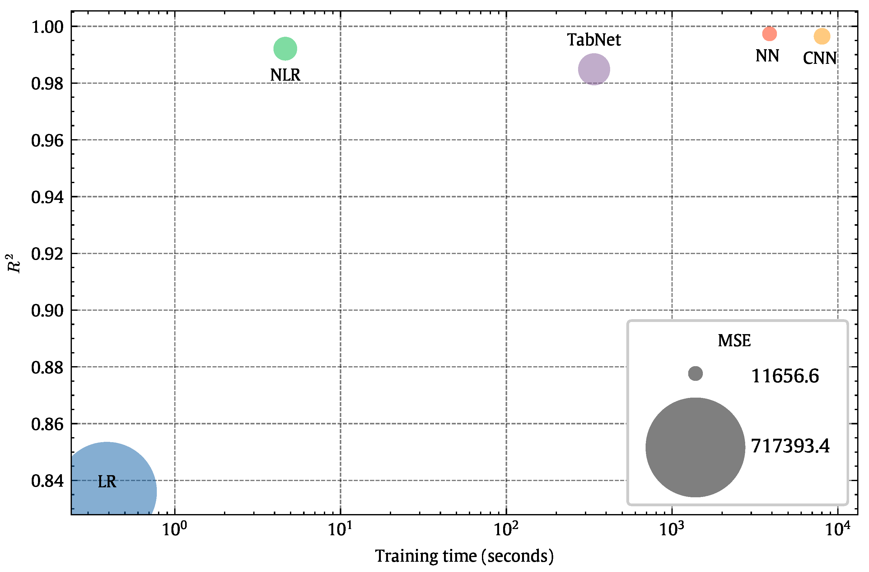
NN	TensorFlow	0.99734	11,656.59	41.75

summarizes the results of the models we tried in ascending order according to accuracy. Figure 20 is a visual representation of the same information in Table 5.

5.3. Reduced Model

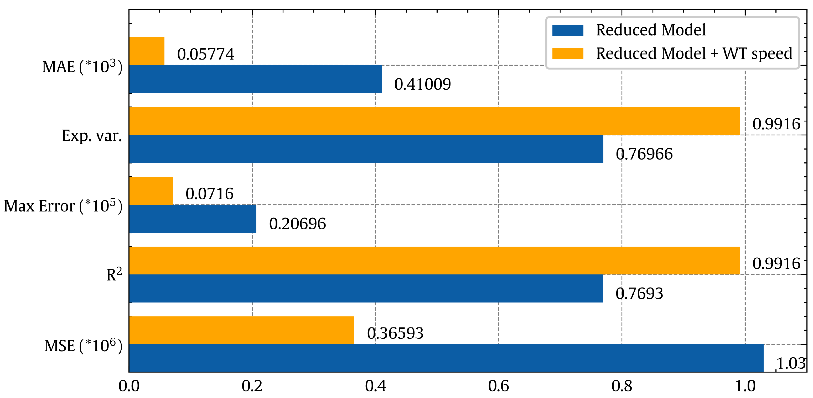
Following the same investigation as [79], we used essential features to make predictions. According to Figure 4, the essential features are the temperature of the outside air [CH1-12], the temperature inside the tower [CH1-13], solar radiation [CH2-1], wind speed of the outside air [CH2-4], thermal updraft [CH2-7], wind direction (at the rotor) [CH2-8]. The power production prediction was not accurate, as we were still missing a feature to represent the wind turbine. After adding the wind turbine speed [CH3-1] as a feature, the prediction improved dramatically, going from R² = 0.7693 to R² = 0.9916. Figure 21 represents a comparison between the results of the reduced feature model (six features) and the model after adding wind turbine speed as an enhancing feature, according to the scores of quality metrics. Both models are based on NN with three hidden layers.

If we compare the numbers of the blue bars (NN, full features) in Figure 19 and orange bars (NN, reduced features + WT speed feature) in Figure 21, we could notice that the decrease in accuracy is not huge, as R² reduced from 0.99734 to 0.9916. This means that the reduced model has slightly lower accuracy than the full-feature model, but it saves significant time and resources by measuring less data.

This sequence of results aims to provide a complete guide for researchers interested in WST, to decide which model is suitable for their case. For instance, researchers who have built a WST prototype but did not use sensors to measure all the possible features can use the reduced model. Other researchers who have high computational power and want more accuracy can use the ANN model, and if they care more about the time instead of the accuracy, they could choose the NLR model, and so on.

6. Conclusions and Future Work

Effective management and feasibility of renewable energy systems as sustainable solutions require accurate power prediction. In this work, we demonstrated machine and deep learning approaches for output power prediction in wind–solar tower systems. We used experimental data from a wind–solar tower prototype designed and established at Kyushu University in Japan. We explored linear and nonlinear multivariate regression models, and then chose suitable models according to several quality metrics as well as the computational cost.

• A simple linear regression model has been used to predict the power output of the WST system. However, despite parameter fine-tuning of the model, the resulting coefficient of determination R², with a value of 0.836, is not sufficiently accurate. This can be explained by the nonlinearity of the wind turbine employed with the WST system.
• A non-linear regression model shall improve the accuracy of prediction. A second-order polynomial regression model was in fact an improvement and the accuracy of prediction measured by R² has increased to an acceptable value of 0.992. The main advantage of the NLR is the acceptable computational time compared to the prediction accuracy.
• For higher accuracy of prediction, network-based DL models can outperform the classical ML methods. Two different DL models were used in this study, namely ANN and 1-D CNN models. ANN was found to be superior to the CNN model in terms of computational and evaluation time cost, and the higher accuracy of prediction with R² of 0.997734 for ANN compared to 0.99647 for CNN.

Among the four models, ANN showed the best capabilities in predicting the power output and can be used with confidence in the feasibility studies to choose the deployment locations, provided that computational power is available. Otherwise, NLR is sufficient, with a slightly lower accuracy in case the computational power is not high enough. Finally, feature reduction has been explored, but while keeping a feature to represent the turbine. This causes a slight reduction in accuracy but with great effort and resource savings.

For future work, we shall explore weather conditions and measurements in order to select suitable locations for WST system deployment such that the power generation is maximized. Also, we plan to enrich our WST power prediction model with additional inputs, including measurements for differentiating between rainy and dry days, as well as factors of natural precipitation inside the WST collector. These additional inputs shall enhance the model’s accuracy for the whole year. ML/DL algorithms could also be used for improving the design of wind–solar towers, through careful investigation of tower design factors, such as the tower inclination angle, the tower height, the diameter of the tower base, the turbine distance from the tower base, etc. Combinations of these factors can be experimentally explored and used to train machine learning models in order to achieve optimal WST design.

References

- Dincer, I.; Acar, C. A review on clean energy solutions for better sustainability. Int. J. Energy Res. 2015, 39, 585–606. [Google Scholar] [CrossRef]
- Carley, S.; Konisky, D.M. The justice and equity implications of the clean energy transition. Nat. Energy 2020, 5, 569–577. [Google Scholar] [CrossRef]
- Rhodes, C.J. The 2015 Paris climate change conference: COP21. Sci. Prog. 2016, 99, 97–104. [Google Scholar] [CrossRef]
- Twidell, J.; Weir, T. Renewable Energy Resources; Routledge: London, UK, 2015. [Google Scholar]
- Kannan, N.; Vakeesan, D. Solar energy for future world: A review. Renew. Sustain. Energy Rev. 2016, 62, 1092–1105. [Google Scholar] [CrossRef]
- Zhu, J.; Su, L.; Li, Y. Wind power forecasting based on new hybrid model with TCN residual modification. Energy AI 2022, 10, 100199. [Google Scholar] [CrossRef]
- Moran, E.F.; Lopez, M.C.; Moore, N.; Müller, N.; Hyndman, D.W. Sustainable hydropower in the 21st century. Proc. Natl. Acad. Sci. USA 2018, 115, 11891–11898. [Google Scholar] [CrossRef] [PubMed]
- Zhou, Y. Ocean energy applications for coastal communities with artificial intelligence a state-of-the-art review. Energy AI 2022, 10, 100189. [Google Scholar] [CrossRef]
- Zarrouk, S.J.; Moon, H. Efficiency of geothermal power plants: A worldwide review. Geothermics 2014, 51, 142–153. [Google Scholar] [CrossRef]
- Khalifa, N.M.; Rezaei, A.S.; Taha, H.E. Comparing the performance of different turbulence models in predicting dynamic stall. In Proceedings of the AIAA Scitech 2021 Forum, Online, 11–15 January 2021; p. 1651. [Google Scholar]
- Pla Olea, L.; Khalifa, N.M.; Taha, H.E. Geometric Control Study of the Beddoes-Leishman Model in a Pitching-Plunging Airfoil. In Proceedings of the AIAA SCITECH 2022 Forum, San Diego, CA, USA, 3–7 January 2022; p. 2415. [Google Scholar]
- Shaheen, M.A.; Ullah, Z.; Qais, M.H.; Hasanien, H.M.; Chua, K.J.; Tostado-Véliz, M.; Turky, R.A.; Jurado, F.; Elkadeem, M.R. Solution of probabilistic optimal power flow incorporating renewable energy uncertainty using a novel circle search algorithm. Energies 2022, 15, 8303. [Google Scholar] [CrossRef]
- Jamali, S.; Nemati, A.; Mohammadkhani, F.; Yari, M. Thermal and economic assessment of a solar chimney cooled semi-transparent photovoltaic (STPV) power plant in different climates. Sol. Energy 2019, 185, 480–493. [Google Scholar] [CrossRef]
- Sharma, S.; Sengar, N. Review of solar PV training manuals and development of survey based solar PV system training formats for beginners. Sol. Energy 2022, 241, 72–84. [Google Scholar] [CrossRef]
- Atiz, A.; Erden, M.; Karakilcik, M. Energy and exergy analyses and electricity generation of PV-T combined with a solar collector for varying mass flow rate and ambient temperature. Heat Mass Transf. 2022, 58, 1263–1278. [Google Scholar] [CrossRef]
- Kizildag, D.; Castro, J.; Kessentini, H.; Schillaci, E.; Rigola, J. First test field performance of highly efficient flat plate solar collectors with transparent insulation and low-cost overheating protection. Sol. Energy 2022, 236, 239–248. [Google Scholar] [CrossRef]
- Koholé, Y.W.; Fohagui, F.C.V.; Tchuen, G. Flat-plate solar collector thermal performance assessment via energy, exergy and irreversibility analysis. Energy Convers. Manag. X 2022, 15, 100247. [Google Scholar]
- Mustafa, J.; Alqaed, S.; Sharifpur, M. Numerical study on performance of double-fluid parabolic trough solar collector occupied with hybrid non-Newtonian nanofluids: Investigation of effects of helical absorber tube using deep learning. Eng. Anal. Bound. Elem. 2022, 140, 562–580. [Google Scholar] [CrossRef]
- Shajan, S.; Baiju, V. Designing a novel small-scale parabolic trough solar thermal collector with secondary reflector for uniform heat flux distribution. Appl. Therm. Eng. 2022, 213, 118660. [Google Scholar] [CrossRef]
- Malik, M.Z.; Shaikh, P.H.; Zhang, S.; Lashari, A.A.; Leghari, Z.H.; Baloch, M.H.; Memon, Z.A.; Caiming, C. A review on design parameters and specifications of parabolic solar dish Stirling systems and their applications. Energy Rep. 2022, 8, 4128–4154. [Google Scholar] [CrossRef]
- Li, X.; Li, R.; Chang, H.; Zeng, L.; Xi, Z.; Li, Y. Numerical simulation of a cavity receiver enhanced with transparent aerogel for parabolic dish solar power generation. Energy 2022, 246, 123358. [Google Scholar] [CrossRef]
- Dhahri, A.; Omri, A. A review of solar chimney power generation technology. Int. J. Eng. Adv. Technol. 2013, 2, 1–17. [Google Scholar]
- Ahmed, O.K.; Hussein, A.S. New design of solar chimney (case study). Case Stud. Therm. Eng. 2018, 11, 105–112. [Google Scholar] [CrossRef]
- Long, T.; Zheng, D.; Li, Y.; Liu, S.; Lu, J.; Shi, D.; Huang, S. Experimental study on liquid desiccant regeneration performance of solar still and natural convective regenerators with/without mixed convection effect generated by solar chimney. Energy 2022, 239, 121919. [Google Scholar] [CrossRef]
- Maia, C.B.; Silva, F.V.; Oliveira, V.L.; Kazmerski, L.L. An overview of the use of solar chimneys for desalination. Sol. Energy 2019, 183, 83–95. [Google Scholar] [CrossRef]
- Kiwan, S.; Salim, I. A hybrid solar chimney/photovoltaic thermal system for direct electric power production and water distillation. Sustain. Energy Technol. Assess. 2020, 38, 100680. [Google Scholar] [CrossRef]
- Li, Z.; Ye, L.; Zhao, Y.; Pei, M.; Lu, P.; Li, Y.; Dai, B. A Spatiotemporal Directed Graph Convolution Network for Ultra-Short-Term Wind Power Prediction. IEEE Trans. Sustain. Energy 2022, 14, 39–54. [Google Scholar] [CrossRef]
- Li, H.; Ren, Z.; Xu, Y.; Li, W.; Hu, B. A multi-data driven hybrid learning method for weekly photovoltaic power scenario forecast. IEEE Trans. Sustain. Energy 2021, 13, 91–100. [Google Scholar] [CrossRef]
- Guo, S.; Liu, Q.; Sun, J.; Jin, H. A review on the utilization of hybrid renewable energy. Renew. Sustain. Energy Rev. 2018, 91, 1121–1147. [Google Scholar] [CrossRef]
- Khare, V.; Nema, S.; Baredar, P. Solar–wind hybrid renewable energy system: A review. Renew. Sustain. Energy Rev. 2016, 58, 23–33. [Google Scholar] [CrossRef]
- Chow, T.T.; Tiwari, G.; Menezo, C. Hybrid solar: A review on photovoltaic and thermal power integration. Int. J. Photoenergy 2012, 2012, 307287. [Google Scholar] [CrossRef]
- Ahmed, O.K.; Algburi, S.; Ali, Z.H.; Ahmed, A.K.; Shubat, H.N. Hybrid solar chimneys: A comprehensive review. Energy Rep. 2022, 8, 438–460. [Google Scholar] [CrossRef]
- Watanabe, K.; Fukutomi, S.; Ohya, Y.; Uchida, T. An Ignored Wind Generates More Electricity: A Solar Updraft Tower to a Wind Solar Tower. Int. J. Photoenergy 2020, 2020, 4065359. [Google Scholar] [CrossRef]
- Wengenmayr, R.; Bührke, T. Renewable Energy: Sustainable Energy Concepts for the Future; John Wiley & Sons: Hoboken, NJ, USA, 2011. [Google Scholar]
- Schlaich, J.; Bergermann, R.; Schiel, W.; Weinrebe, G. Design of commercial solar updraft tower systems—Utilization of solar induced convective flows for power generation. J. Sol. Energy Eng. 2005, 127, 117–124. [Google Scholar] [CrossRef]
- Richards, R. Spanish solar chimney nears completion. MPS Rev. 1981, 6, 21–23. [Google Scholar]
- Haaf, W.; Friedrich, K.; Mayr, G.; Schlaich, J. Solar chimneys part I: Principle and construction of the pilot plant in Manzanares. Int. J. Sol. Energy 1983, 2, 3–20. [Google Scholar] [CrossRef]
- Haaf, W. Solar chimneys: Part ii: Preliminary test results from the Manzanares pilot plant. Int. J. Sustain. Energy 1984, 2, 141–161. [Google Scholar] [CrossRef]
- Jafarifar, N.; Behzadi, M.M.; Yaghini, M. The effect of strong ambient winds on the efficiency of solar updraft power towers: A numerical case study for Orkney. Renew. Energy 2019, 136, 937–944. [Google Scholar] [CrossRef]
- Okada, S.; Uchida, T.; Karasudani, T.; Ohya, Y. Improvement in solar chimney power generation by using a diffuser tower. J. Sol. Energy Eng. 2015, 137. [Google Scholar] [CrossRef]
- Mebarki, A.; Sekhri, A.; Assassi, A.; Hanafi, A.; Marir, B. CFD analysis of solar chimney power plant: Finding a relationship between model minimization and its performance for use in urban areas. Energy Rep. 2022, 8, 500–513. [Google Scholar] [CrossRef]
- Eryener, D.; Kuscu, H. Hybrid transpired solar collector updraft tower. Sol. Energy 2018, 159, 561–571. [Google Scholar] [CrossRef]
- Boretti, A. Integration of solar thermal and photovoltaic, wind, and battery energy storage through AI in NEOM city. Energy AI 2021, 3, 100038. [Google Scholar] [CrossRef]
- Yapıcı, E.Ö.; Ayli, E.; Nsaif, O. Numerical investigation on the performance of a small scale solar chimney power plant for different geometrical parameters. J. Clean. Prod. 2020, 276, 122908. [Google Scholar] [CrossRef]
- Hamdan, M.O. Analysis of a solar chimney power plant in the Arabian Gulf region. Renew. Energy 2011, 36, 2593–2598. [Google Scholar] [CrossRef]
- Li, J.; Guo, P.; Wang, Y. Preliminary investigation of a novel solar and wind energy extraction system. Proc. Inst. Mech. Eng. Part A J. Power Energy 2012, 226, 73–85. [Google Scholar] [CrossRef]
- Zuo, L.; Ding, L.; Chen, J.; Zhou, X.; Xu, B.; Liu, Z. Comprehensive study of wind supercharged solar chimney power plant combined with seawater desalination. Sol. Energy 2018, 166, 59–70. [Google Scholar] [CrossRef]
- Anbarasi, J.; Rajamurugu, N.; Yaknesh, S. Optimizing the collector inlet height of a divergent solar tower using response surface methodology. Mater. Today Proc. 2022, 55, 404–413. [Google Scholar] [CrossRef]
- Das, P.; Chandramohan, V. 3D numerical study on estimating flow and performance parameters of solar updraft tower (SUT) plant: Impact of divergent angle of chimney, ambient temperature, solar flux and turbine efficiency. J. Clean. Prod. 2020, 256, 120353. [Google Scholar] [CrossRef]
- Kebabsa, H.; Lounici, M.S.; Daimallah, A. Numerical investigation of a novel tower solar chimney concept. Energy 2021, 214, 119048. [Google Scholar] [CrossRef]
- Kebabsa, H.; Lounici, M.S.; Lebbi, M.; Daimallah, A. Thermo-hydrodynamic behavior of an innovative solar chimney. Renew. Energy 2020, 145, 2074–2090. [Google Scholar] [CrossRef]
- Praveen, V.; Das, P.; Chandramohan, V. A novel concept of introducing a fillet at the chimney base of solar updraft tower plant and thereby improving the performance: A numerical study. Renew. Energy 2021, 179, 37–46. [Google Scholar] [CrossRef]
- Li, J.-Y.; Guo, P.-H.; Wang, Y. Effects of collector radius and chimney height on power output of a solar chimney power plant with turbines. Renew. Energy 2012, 47, 21–28. [Google Scholar] [CrossRef]
- Das, P.; Chandramohan, V. Experimental studies of a laboratory scale inclined collector solar updraft tower plant with thermal energy storage system. J. Build. Eng. 2021, 41, 102394. [Google Scholar] [CrossRef]
- Murena, F.; Gaggiano, I.; Mele, B. Fluid dynamic performances of a solar chimney plant: Analysis of experimental data and CFD modelling. Energy 2022, 249, 123702. [Google Scholar] [CrossRef]
- Das, P.; Chandramohan, V. Estimation of flow parameters and power potential of solar vortex engine (SVE) by varying its geometrical configurations: A numerical study. Energy Convers. Manag. 2020, 223, 113272. [Google Scholar] [CrossRef]
- Ghenai, C.; Ahmad, F.F.; Rejeb, O.; Bettayeb, M. Artificial neural networks for power output forecasting from bifacial solar PV system with enhanced building roof surface Albedo. J. Build. Eng. 2022, 56, 104799. [Google Scholar] [CrossRef]
- Abdelsalam, E.; Darwish, O.; Karajeh, O.; Almomani, F.; Darweesh, D.; Kiswani, S.; Omar, A.; Kisrawi, M. A classifier to detect best mode for Solar Chimney Power Plant system. Renew. Energy 2022, 197, 244–256. [Google Scholar] [CrossRef]
- Ayyad, M.; Hajj, M.R.; Marsooli, R. Artificial intelligence for hurricane storm surge hazard assessment. Ocean Eng. 2022, 245, 110435. [Google Scholar] [CrossRef]
- Fateen, M.; Mine, T. Predicting Student Performance Using Teacher Observation Reports. In Proceedings of the 14th International Conference on Educational Data Mining (EDM), Online, 29 June–2 July 2021. [Google Scholar]
- Liu, H.; Zhang, Z. A Bi-party Engaged Modeling Framework for Renewable Power Predictions with Privacy-preserving. IEEE Trans. Power Syst. 2022, 38, 5794–5805. [Google Scholar] [CrossRef]
- Liu, H.; Yang, L.; Zhang, B.; Zhang, Z. A two-channel deep network based model for improving ultra-short-term prediction of wind power via utilizing multi-source data. Energy 2023, 283, 128510. [Google Scholar] [CrossRef]
- Liu, H.; Zhang, Z. A bilateral branch learning paradigm for short term wind power prediction with data of multiple sampling resolutions. J. Clean. Prod. 2022, 380, 134977. [Google Scholar] [CrossRef]
- Voyant, C.; Notton, G.; Kalogirou, S.; Nivet, M.L.; Paoli, C.; Motte, F.; Fouilloy, A. Machine learning methods for solar radiation forecasting: A review. Renew. Energy 2017, 105, 569–582. [Google Scholar] [CrossRef]
- Cattani, G. Combining data envelopment analysis and Random Forest for selecting optimal locations of solar PV plants. Energy AI 2023, 11, 100222. [Google Scholar] [CrossRef]
- Kalogirou, S. Artificial Intelligence in Energy and Renewable Energy Systems; Nova Publishers: Hauppauge, NY, USA, 2007. [Google Scholar]
- Patil, S.; Dhoble, A.; Sathe, T.; Thawkar, V. Predicting Performance of Solar updraught Tower Using Machine Learning Regression Model. Aust. J. Mech. Eng. 2023, 1–19. [Google Scholar] [CrossRef]
- Wang, J.; Guo, L.; Zhang, C.; Song, L.; Duan, J.; Duan, L. Thermal power forecasting of solar power tower system by combining mechanism modeling and deep learning method. Energy 2020, 208, 118403. [Google Scholar] [CrossRef]
- Dubey, A.K.; Kumar, A.; Ramirez, I.S.; Marquez, F.P.G. A Review of Intelligent Systems for the Prediction of Wind Energy Using Machine Learning. In Proceedings of the International Conference on Management Science and Engineering Management, Ankara, Turkey, 3–6 August 2022; Springer: Berlin/Heidelberg, Germany, 2022; pp. 476–491. [Google Scholar]
- Shakibi, H.; Assareh, E.; Chitsaz, A.; Keykhah, S.; Behrang, M.; Golshanzadeh, M.; Ghodrat, M.; Lee, M. Exergoeconomic and optimization study of a solar and wind-driven plant employing machine learning approaches; a case study of Las Vegas city. J. Clean. Prod. 2023, 385, 135529. [Google Scholar] [CrossRef]
- Li, M.; Liu, Y.; Liu, X.; Sun, Q.; You, X.; Yang, H.; Luan, Z.; Gan, L.; Yang, G.; Qian, D. The deep learning compiler: A comprehensive survey. IEEE Trans. Parallel Distrib. Syst. 2020, 32, 708–727. [Google Scholar] [CrossRef]
- Géron, A. Hands-On Machine Learning with Scikit-Learn, Keras, and TensorFlow: Concepts, Tools, and Techniques to Build Intelligent Systems, 2nd ed.; O’Reilly Media: Sevastopol, CA, USA, 2019. [Google Scholar]
- Borisov, V.; Leemann, T.; Seßler, K.; Haug, J.; Pawelczyk, M.; Kasneci, G. Deep neural networks and tabular data: A survey. IEEE Trans. Neural Netw. Learn. Syst. 2022, 35, 7499–7519. [Google Scholar] [CrossRef]
- Chang, Y.; Wang, X.; Wang, J.; Wu, Y.; Yang, L.; Zhu, K.; Chen, H.; Yi, X.; Wang, C.; Wang, Y.; et al. A survey on evaluation of large language models. ACM Trans. Intell. Syst. Technol. 2023, 15, 1–45. [Google Scholar] [CrossRef]
- Chen, T.; Guestrin, C. Xgboost: A scalable tree boosting system. In Proceedings of the 22nd acm sigkdd International Conference on Knowledge Discovery and Data Mining, San Francisco, CA, USA, 13–17 August 2016; pp. 785–794. [Google Scholar]
- Shwartz-Ziv, R.; Armon, A. Tabular data: Deep learning is not all you need. Inf. Fusion 2022, 81, 84–90. [Google Scholar] [CrossRef]
- Pasumarthi, N.; Sherif, S. Experimental and theoretical performance of a demonstration solar chimney model—Part II: Experimental and theoretical results and economic analysis. Int. J. Energy Res. 1998, 22, 443–461. [Google Scholar] [CrossRef]
- Ohya, Y.; Wataka, M.; Watanabe, K.; Uchida, T. Laboratory experiment and numerical analysis of a new type of solar tower efficiently generating a thermal updraft. Energies 2016, 9, 1077. [Google Scholar] [CrossRef]
- Rushdi, M.A.; Yoshida, S.; Watanabe, K.; Ohya, Y. Machine Learning Approaches for Thermal Updraft Prediction in Wind Solar Tower Systems. Renew. Energy 2021, 177, 1001–1013. [Google Scholar] [CrossRef]
- Oka, N.; Furukawa, M.; Kawamitsu, K.; Yamada, K. Optimum aerodynamic design for wind-lens turbine. J. Fluid Sci. Technol. 2016, 11, JFST0011. [Google Scholar] [CrossRef]
- Matsumiya, H.; Tsutsui, Y.; Kawamura, S.; Kieda, K.; Kato, E.; Takano, S.; Toe, Y. Performance of New ‘MEL-WING SECTIONS’for Wind Turbines. In Proceedings of the European Community Wind Energy Conference, Madrid, Spain, 10–14 September 1990; pp. 10–14. [Google Scholar]
- Obase, Y.; Hiratani, F.; Furukawa, M. Development of Wind Lens Turbine by Three-Dimension Blade Design. In Proceedings of the Annual Meeting, Japan Society of Fluid Mechanics, Kobe, Japan, 4–7 September 2008; The Japan Society of Fluid Mechanics: Tokyo, Japan, 2008; p. 150. (In Japanese). [Google Scholar]
- Goodfellow, I.; Bengio, Y.; Courville, A. Deep Learning; MIT Press: Cambridge, MA, USA, 2016. [Google Scholar]
- Ruder, S. An overview of gradient descent optimization algorithms. arXiv 2016, arXiv:1609.04747. [Google Scholar]
- Vanhoucke, V.; Senior, A.; Mao, M.Z. Improving the speed of neural networks on CPUs. Proc. Deep. Learn. Unsupervised Feature Learn. Nips Workshop 2011, 1, 4. [Google Scholar]
- Nwankpa, C.E.; Ijomah, W.; Gachagan, A.; Marshall, S. Activation functions: Comparison of trends in practice and research for deep learning. In Proceedings of the 2nd International Conference on Computational Sciences and Technology, Mohali, India, 17–18 December 2021; pp. 124–133. [Google Scholar]
- Pedregosa, F.; Varoquaux, G.; Gramfort, A.; Michel, V.; Thirion, B.; Grisel, O.; Blondel, M.; Prettenhofer, P.; Weiss, R.; Dubourg, V.; et al. Scikit-learn: Machine learning in Python. J. Mach. Learn. Res. 2011, 12, 2825–2830. [Google Scholar]
- Scikit-Learn Developers. Tuning the Hyper-Parameters of an Estimator. Available online: https://scikit-learn.org/stable/modules/grid_search.html (accessed on 9 September 2021).
- Chollet, F. Keras. 2015. Available online: https://keras.io (accessed on 23 July 2024).
- Kingma, D.P.; Ba, J. Adam: A method for stochastic optimization. arXiv 2014, arXiv:1412.6980. [Google Scholar]
- Prechelt, L. Automatic early stopping using cross validation: Quantifying the criteria. Neural Netw. 1998, 11, 761–767. [Google Scholar] [CrossRef]
- Nusrat, I.; Jang, S.B. A comparison of regularization techniques in deep neural networks. Symmetry 2018, 10, 648. [Google Scholar] [CrossRef]
- Srivastava, N.; Hinton, G.; Krizhevsky, A.; Sutskever, I.; Salakhutdinov, R. Dropout: A simple way to prevent neural networks from overfitting. J. Mach. Learn. Res. 2014, 15, 1929–1958. [Google Scholar]
- Arik, S.Ö.; Pfister, T. Tabnet: Attentive interpretable tabular learning. In Proceedings of the AAAI Conference on Artificial Intelligence, Virtually, 2–9 February 2021; Volume 35, pp. 6679–6687. [Google Scholar]
Figure 1.
A schematic illustration of the power generation process in the wind–solar towers [
33].
Figure 2.
Sensor locations within the WST system [
79].
Figure 3.
Heatmap visualization of the pairwise correlation for all pairs of WST input features based on the PCC.
Figure 4.
Bar chart of the absolute values of the PCCs between the output power [CH3-2] and each of the WST input features.
Figure 5.
An artificial neural network for single output prediction with 2 hidden layers.
Figure 6.
The representation of a single neuron for the jth node in the lth layer of a neural network architecture.
Figure 7.
Illustration of main components of ConvNets (numbers are just for example to show conve and pooling operations). Note that the * symbol represents the convolutional operation.
Figure 8.
True values vs. predicted values of the LR model.
Figure 9.
Histogram of the prediction error of the LR model.
Figure 10.
Temporal patterns of the true power output [CH3-2] values (blue line) and the corresponding predicted values (orange line) for the linear regression model on the validation set.
Figure 11.
Power prediction performance comparison between the linear regression and fine-tuned ridge regression models based on several quality metrics.
Figure 12.
True values vs. predicted values of the non-linear regression model.
Figure 13.
Histogram of the prediction error of the non-linear regression model.
Figure 14.
Temporal patterns of the true power output [CH3-2] values (blue) and the corresponding predicted values (orange) for the non-linear polynomial regression model on the validation set.
Figure 15.
Heatmap visualization of the tuning of dropout and regularization, based on R2 quality metric.
Figure 16.
Evolution of the MSE-based training and test losses (learning curve) of the proposed deep learning model for WST output power prediction.
Figure 17.
True values vs. predicted values of the NN model.
Figure 18.
Temporal patterns of the true power output [CH3-2] values (blue line) and the corresponding predicted values (orange line) for the deep learning model on the validation set.
Figure 19.
Power prediction performance comparison between a neural network with 3 hidden layers and 1-D convolutional neural network models based on several quality metrics.
Figure 20.
Visual performance comparison according to , MSA, training time.
Figure 21.
Power prediction performance comparison between reduced feature model and model after adding wind turbine speed feature, based on several quality metrics.