Article

An Early Warning Model for Turbine Intermediate-Stage Flux Failure Based on an Improved HEOA Algorithm Optimizing DMSE-GRU Model

1
State Power Investment Inner Mongolia Energy Co., Ltd., Hohhot 010020, China
2
Shanghai Power Equipment Research Institue Co., Ltd., Shanghai 200240, China
3
Key Laboratory of Energy Thermal Conversion and Control of Ministry of Education, School of Energy and Environment, Southeast University, Nanjing 210096, China
*
Author to whom correspondence should be addressed.
Energies 2024, 17(15), 3629; https://doi.org/10.3390/en17153629
Submission received: 24 May 2024 / Revised: 27 June 2024 / Accepted: 5 July 2024 / Published: 24 July 2024
(This article belongs to the Section F1: Electrical Power System)

Abstract

:
As renewable energy sources such as wind and photovoltaics continue to enter the grid, their intermittency and instability leads to an increasing demand for peaking and frequency regulation. An efficient dynamic monitoring method is necessary to improve the safety level of intelligent operation and maintenance of power stations. To overcome the insufficient detection accuracy and poor adaptability of traditional methods, a novel fault early warning method with careful consideration of dynamic characteristics and model optimization is proposed. A combined loss function is proposed based on the dynamic time warping and the mean square error from the perspective of both shape similarity and time similarity. A prediction model of steam turbine intermediate-stage extraction temperature based on the gate recurrent unit is then proposed, and the change in prediction residuals is utilized as a fault warning criterion. In order to further improve the diagnostic accuracy, a human evolutionary optimization algorithm with lens opposition-based learning is proposed for model parameter adaptive optimization. Experiments on real-world normal and faulty operational data demonstrate that the proposed method can improve the detection accuracy by an average of 1.31% and 1.03% compared to the long short-term memory network, convolutional neural network, back propagation network, extreme learning machines, gradient boosting decision tree, and LightGBM models.

1. Introduction

With the gradual increase in the penetration ratio of renewable energy, thermal power units will be under deep and fast peak and frequency regulation operating conditions [1]. Compared with the traditional steady-state operating conditions, frequent, rapid, and wide-ranging load changes will exacerbate or trigger safety hazards [2,3]. The main reasons include thermal fatigue and damage due to thermal stress alternation and increased wear of devices due to frequent equipment operation [4,5]. Health state management and real-time fault monitoring are important methods to improve the safe and reliable operation of in-service steam turbine units [6,7,8]. This research topic investigates the turbine operating condition fault early warning method and strengthens the monitoring of the turbine unit equipment [9]. The development of fault detection technology helps to improve the reliability of unit operation and is important for improving the stability of the entire power system.
As the core thermal power conversion equipment of the thermal power unit machine, the performance of the turbine intermediate-stage flux section directly affects the overall performance of the unit. Under the high rotor speed, problems such as vapor excitation and rotor unbalance may occur. The realization of accurate performance monitoring and sensitive early warning of the turbine flow section is of great significance to ensure the safe and stable operation of the turbine. As an extremely complex piece of power equipment, the turbine has a large number of inertial links for energy and value storage, so the traditional fixed-threshold diagnostic method is unable to realize the demand for early warning. Extracting anomalous features using machine learning methods is an effective approach, and there are some partially relevant studies. Salahshoor et al. [10] proposed a turbine fault detection and diagnosis model based on the support vector machine and adaptive neuro-fuzzy inference system. Hashmi et al. [11] proposed a turbine fault diagnostics approach based on artificial neural networks (ANNs). Although the above methods have achieved high fault diagnosis accuracy, their practicality is insufficient. Firstly, actual fault data are difficult to obtain, resulting in fault classifiers not being trained. Compared to the diagnosis of faults after they have occurred, alarms in the early stages of faults are more meaningful. Meanwhile, the measurement signals of the turbine operation process have strong dynamic information, and it is difficult for the static neural network to extract the time features effectively. Recurrent neural networks (RNNs) and their variants rely on a special recurrent structure within them to process historical information [12]. Only a few researchers have focused on these issues. Li et al. [13] proposed a flux fault early warning method based on the long short-term memory (LSTM) model. However, the current research on fault detection methods that consider timing information is very insufficient. The issue of how to improve the accuracy of anomaly detection by extracting normal data temporal information is the first problem to be addressed in this paper.
Frequent and wide-ranging variable condition operation of thermal power units can lead to drastic parameter fluctuations. Ordinary neural networks are difficult to accurately predict and detect the state of target parameters [14]. The performance of a predictive model depends on the hiding state of the neurons in the neural network and its hidden layers, as it helps to determine the efficiency of the model [15]. Manual tuning of hyperparameters is an essential step in machine learning during neural network modeling [16]. Regarding this issue, the use of global optimization algorithms is an effective approach, such as particle swarm optimization (PSO) [17], grey wolf optimizer (GWO) [18], and so on. Olayode et al. [19] found that the ANN-PSO method is more efficient and simpler than generic neural networks. Abou et al. [20] proposed a coati optimization algorithm-based hybrid deep learning model for wind power forecasting. The optimization of neural networks is slow and complex, which must require optimization algorithms with powerful search capabilities. Qin et al. [21] improved PSO by introducing bounding rebound strategy to optimize the Bayesian model. How to make effective improvements to the existing methods so as to increase the optimization efficiency is the second problem to be addressed.
In addition to using dynamic models and optimization algorithms, customizing the loss function is an effective method and has been studied by some scholars in other fields of prediction tasks. Li et al. [22] proposed a Cauchy loss function for time series prediction to enhance robustness against noise and introduced lasso regression (L1) regularization to smooth the slope. He et al. [23] proposed a segmented asymmetric loss function for thrust prediction during rocket failures to prevent positive error. Combining various loss functions is an effective method. Zhou et al. [24] proposed a loss function consisting of mean squared error (MSE), asymmetric function and L1 regularization for gas turbine degradation trend prediction. For the turbine temperature prediction and anomaly detection problem studied in this paper, the above custom loss function is not applicable. To make the prediction results similar to the actual suppression, the similarity of the prediction results should also be ensured. Dynamic time warping (DTW) is an effective method for calculating sequence similarity, which is widely used in areas such as speech recognition [25], time series data mining [26], and bioinformatics [27]. Li et al. [28] applied DTW to power prediction. Zhou et al. [29] used DTW in a similarity assessment for evaluating the operating signals of an aero-engine. DTW is a method for evaluating the similarity distance of the operating signals of an aero-engine. DTW shows promise in being used to improve the reasonableness of turbine parameter prediction results. The issue of how it can play a role in turbine temperature prediction and anomaly detection is the key question that needs to be explored in this paper.
To address the existing fault warning models with a simple training process and insufficient prediction accuracy, a turbine intermediate-stage flux fault warning model based on the improved human evolutionary optimization algorithm (HEOA) optimized GRU model is proposed. Meanwhile, a combined loss function based on dynamic time warping and mean squared error (DMSE) is innovatively proposed. The sensitive detection of state changes is achieved based on the Pauta criterion and post-stage temperature changes. The actual data validation in the case unit shows that sensitive fault diagnosis is realized. The main contributions of this paper are as follows.
(1)
A turbine post-stage temperature prediction model based on the GRU model is proposed. The intermediate-stage flux fault detection model is implemented based on the prediction output and actual data error.
(2)
An improved HEOA algorithm based on lens opposition-based learning is proposed. The algorithm is used for the adaptive optimization of GRU model parameters, and higher prediction accuracy is achieved.
(3)
A combined loss function based on dynamic time warping and MSE is proposed. The loss function is utilized to ensure high accuracy and similarity of the model’s predicted trends.
(4)
Fault detection experiments on real data demonstrate that the proposed method achieves optimal detection accuracy. The fault diagnosis accuracy of the proposed model is significantly higher than that of the traditional model and has the lowest false detection rate.
The structure of this article is as follows. Section 2 introduces the technical route proposed and then explains the method principles. Section 3 conducts a gas turbine intermediate-stage flux failure warning experiment using actual data. This section also conducts comparative experiments between different methods. Section 4 summarizes the work conducted and provides plans.

2. Methodology and Principles

2.1. Failure Early Warning Model

The essence of early failure warning is to find the invariants in the changes and judge whether the equipment fails according to the invariants. Accordingly, a new early warning method is proposed to evaluate the performance and monitor the degradation failure with the intrinsic relationship between parameters as performance characterization. Y represents the performance characterization parameters. F represents the state functions of the equipment itself. X is the set of measurement parameters. θ represents the structural parameters of the equipment when the performance of the equipment changes. The process is shown in Equation (1).
Y 0 = F ( X 0 , θ 0 ) Y 1 = F ( X 1 , θ 1 )
where Y 0 and Y 1 are the initial performance and the performance after degradation, respectively.
According to the analysis of equipment failure characterization, F is defined as the constant mode and Y is defined as the constant mode model. The Pauta criterion is used in this study to recognize the early weak signs of failure. The 3 σ , 3 σ of the training set error is defined as the fault detection threshold [13]. When the test set testing error does not exceed this threshold, the unit operates normally. Otherwise, the unit is judged to have performance degradation.

2.2. GRU-Based Constant Mode Fault Warning Model

The GRU network structure is shown in Figure 1. Unlike the simple network structure of RNN, GRU introduces two gating units for selective storing and forgetting of the input information, which are the reset gate and update gate [30].
The realization process is shown in Equation (2).
r t = σ W r · [ h t 1 , x t ] z t = σ W z · [ h t 1 , x t ]
where σ is the sigmoid function, h t 1 is the cell state at the previous time, x t is the input value at the current time, W r is the weight parameter of the reset gate, and W z is the weight parameter of the update gate.
After obtaining the reset factor r t , the reset gate’s gating signal is multiplied with h t 1 and then combined with the input. The data are converted into (−1, 1) using the tanh function to obtain the candidate state of the chosen cell h ˜ t . Finally, the input information is updated by update factor z t of the update gate. This function can be written as Equation (3).
h ˜ t = tanh W h · [ r t h t 1 , x t ] h t = ( 1 z t ) h t 1 + z t h ˜ t
where W h denotes the weight parameter of the choice set.
This mainly includes three stages: input data reset, memorizing the current state, and forgetting and selecting the memory. Compared with LSTM, the effect of GRU is not much different, but its calculation is simpler and the model training is more efficient. The process of fault detection based on GRU model prediction error and Pauta criterion is shown in Equation (4).
Y ^ = W f h t + b f I f Y ^ Y 3 σ N o r m a l I f Y ^ Y > 3 σ A b n o r m a l
where W f and b f are parameters of a fully connected network. Y ^ denotes the forecast value.

2.3. Improved Human Evolutionary Optimization Algorithm

The HEOA is a metaheuristic algorithm inspired by human evolution [31]. HEOA divides the global search process into two distinct phases: human exploration and human development. Initialization using logical chaos mapping. Dividing the optimization phase into a human exploration phase and a human development phase, the initial global search is performed in the first phase. The main principle of the process is shown in Equation (5):
X i t + 1 = β ( 1 t M a x i t e r ) ( X i t X b e s t ) L e v y dim + X b e s t ( 1 t M a x i t e r ) + ( X m e a n t X b e s t ) f l o o r ( r a n d j u m p ) j u m p
where β is the adaptive function, and dim signifies the dimensionality of the problem. X i t denotes the current position, while X i t + 1 signifies the position of the subsequent update. X b e s t corresponds to the best position explored thus far, and X m e a n t represents the average position within the current population. The term f l o o r refers to the operation of rounding downwards. L e v y denotes the L e v y distribution [32], and f j u m p is the jump coefficient.
In the second phase, the population is categorized into leaders, explorers, followers, and losers, each using a different search strategy. In the case of leaders, the mathematical expression is defined as Equation (6).
X i t + 1 = ω X i t exp ( t r a n d n · M a x i t e r ) , R < A ω X i t + R n · o n e s ( 1 , d i m ) , R A
In Equation (6), r a n d n is a random number in the range of [0, 1]. The function o n e s ( 1 , d i m ) generates a row vector, where each element is set to 1. R n is a random number that represents the complexity of the situation associated with the leaders. A = 0.6 denotes the evaluation value of the situation. The knowledge acquisition ease coefficient, denoted as ω , gradually decreases as development progresses.
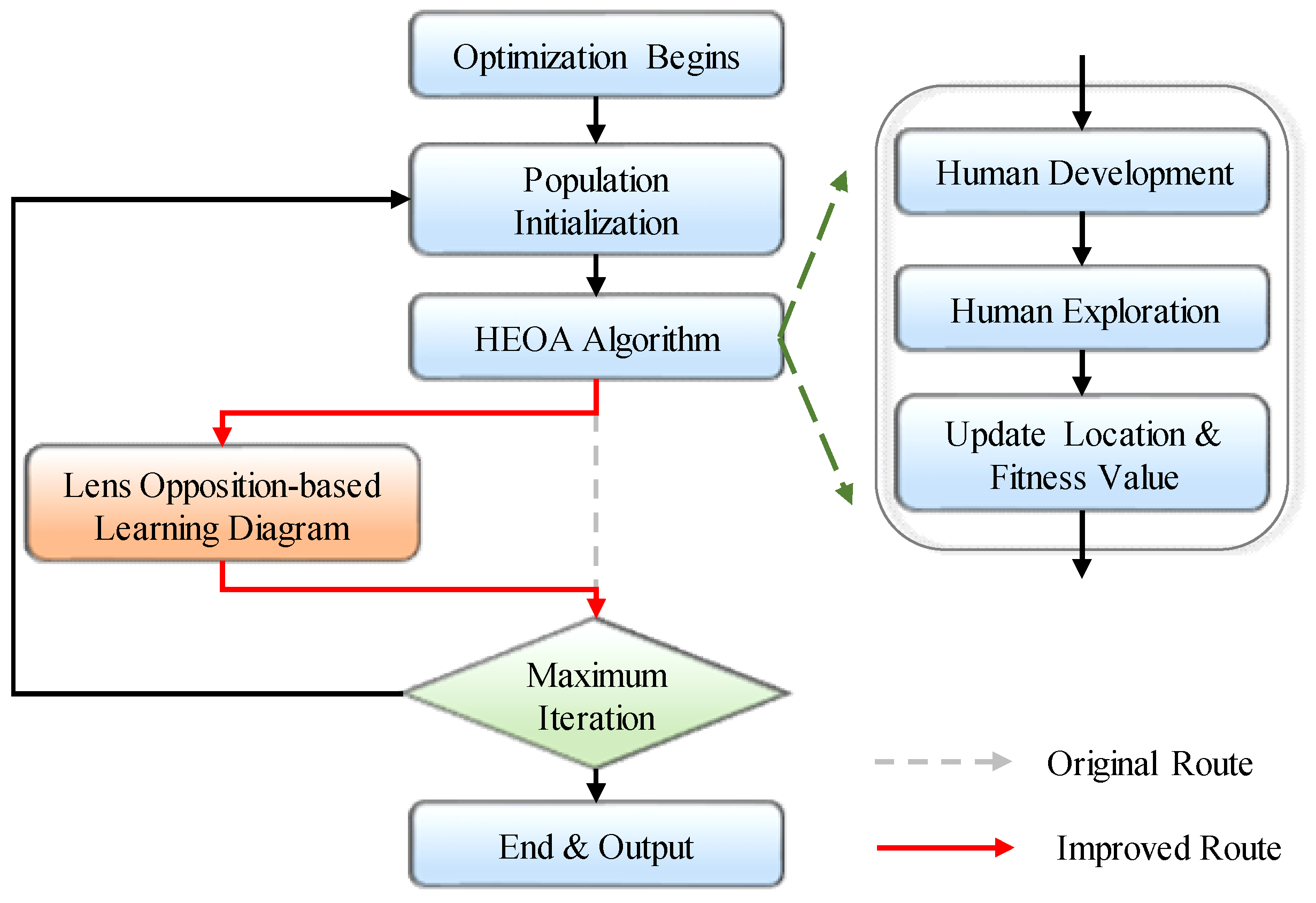
HEOA has an efficient search function, but its transition process between two stages is too simple and can still be further enhanced. The evolutionary directions of different stages of human evolution in nature should be complex and diverse, so this paper adopts the lens opposition-based learning to improve the complexity and learning ability of stage transition [33]. The main idea of lens opposition-based learning comes from the principle of convex lens imaging, which can be seen in Figure 2.
In Figure 2, x takes o as the base point to obtain its corresponding reverse point x , which can be obtained from the lens imaging principle. Let k = h / h to obtain Equation (7) based on lens opposition-based learning.
X i = k + 1 a i + b i / 2 k + X i / k
where X i is the original position and X i is the inverse solution. a i and b i are the maximum and minimum boundaries in the search space.
All the optimized positions obtained by the HEOA are extended using Equation (7) to improve the search capability. The learning process of the improved HEOA (IHEOA) algorithm is shown in Figure 3.

2.4. DMSE Loss Function

The traditional MSE loss function only focuses on the Euclidean distance between the predicted and actual values and does not focus on the shape similarity between the predicted results y ^ and actual results y . The MSE is defined as Equation (8).
M S E = 1 N i = 1 y i y ^ i 2
where N denotes the sample size.
When thermal power units have an inertial link with a large amount of stored energy storage value, there will be a certain time-delay relationship between its operating parameters. The dynamic response between the intermediate-level flux input and output is not real-time correspondence. Therefore, while ensuring the prediction accuracy, the shape of the predicted sequence should also be ensured to be similar. Therefore, the dynamic response process conforms to the actual unit dynamic process.
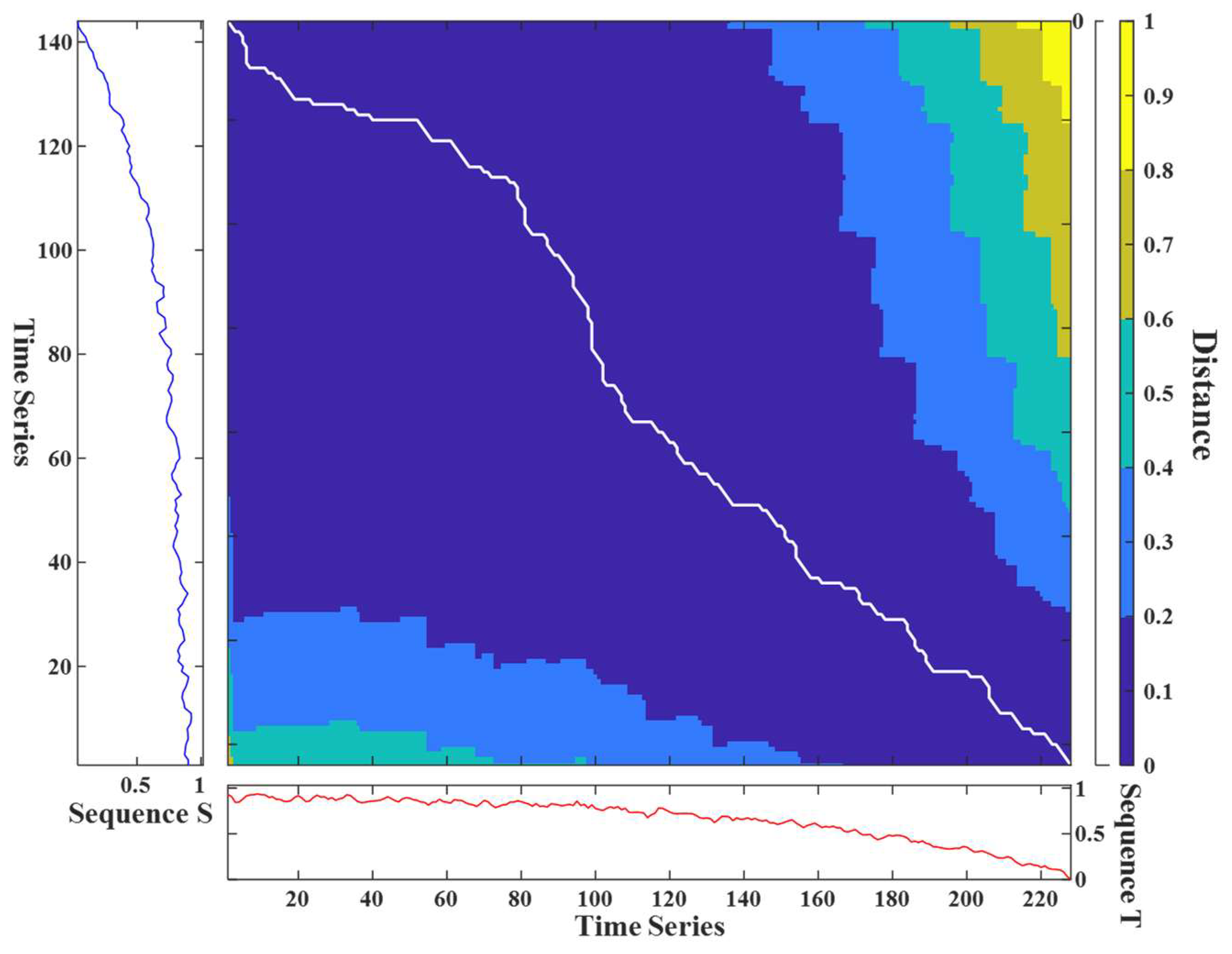
DTW is a similarity assessment method, the principle of which is shown in Figure 4.
First, given two time series T = [ t 1 , t 2 , , t m ] and S = [ s 1 , s 2 , , s n ] , calculate the Euclidean distance d i j of each point and store it in a matrix m × n . The different distances in this matrix can be used to calculate the paths to obtain W = [ w 1 , w 2 , , w k ] . Select the path that satisfies the conditions shown in Equation (9).
max { m , n } < k m + n 1 w 1 = d 11 , w k = d m n w n = d i j , w n + 1 = d p q
These constraints ensure the boundary conditions, monotonicity, and continuity of the warped paths. The final DTW distance of the two sequences is shown in Equation (10).
D T W ( T , S ) = min k = 1 k w k k
The proposed loss function is defined as Equation (11).
D M S E = M S E + D T W
By combining the DTW and MSE functions, the network output values are made to be simultaneously shape and time accurate, which provides a basis for subsequent fault warning.

2.5. Framework

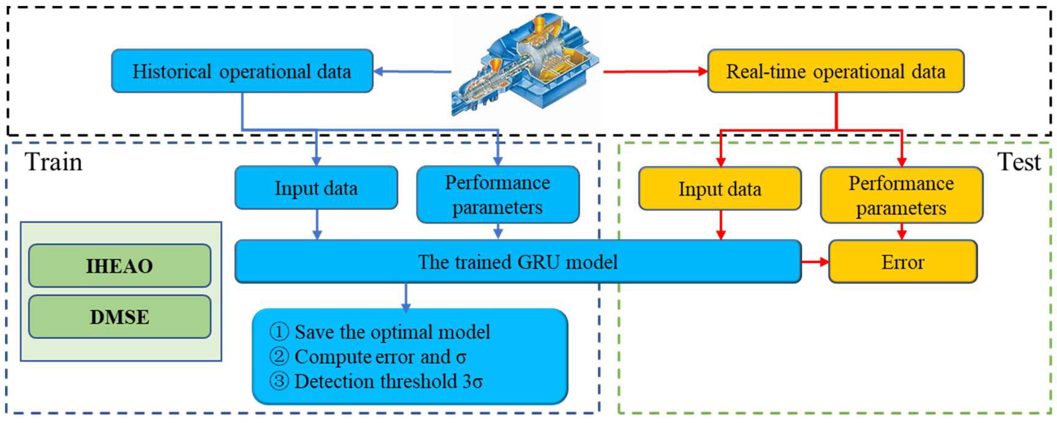
The resulting methodological framework is shown in Figure 5.
The specific implementation process of the method is as follows:
(1)
Data processing: data acquisition and division of training set and test set.
(2)
Model training: set the initial structure of the GRU model, use DMSE as the loss function, use the IHEOA optimization algorithm for parameter optimization, and save the most additive model.
(3)
Fault warning: calculate the fault warning threshold according to the training results and conduct fault warning experiments using test data.

3. Anomaly Detection Experimental Results

3.1. Data Introduction

The experimental data were adopted from the actual operation data of a 660 MW turbine in China, with a total collection time of 636,583 s. The unit load change during this period is shown in Figure 6. The first 491,211 s of data were selected for model training. The middle 71,007 s of data were used for model testing in normal mode. The final 74,365 s of data were used as the second segment of test data. At the 30,000th second of this data segment, there was a sudden failure of the turbine intermediate-stage flux resulting in a 1% increase in temperature.
The prediction accuracy metric used during the experiment was RMSE, which was calculated as the root square of MSE.

3.2. IHEOA Optimization Effect

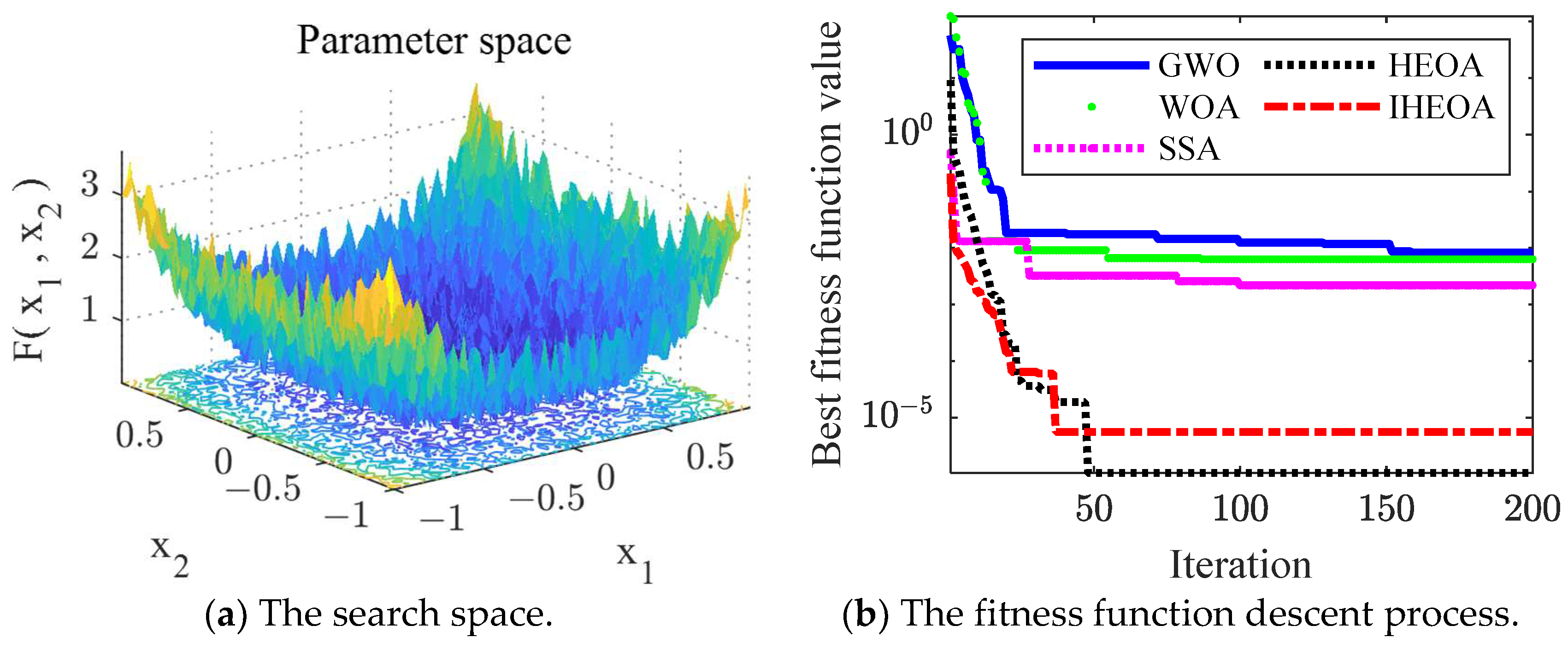
In order to reflect the improvement effect of the HEOA optimization algorithm, improved based on the lens opposition-based learning, the Quartic function with noise in the general 23 test functions of the International Evolutionary Computation CEC was used to carry out the parameter optimization search experiment [34]. The Quartic function is defined as shown in Equation (12).
F x = i = 1 n i x 4 + r a n d n 0 , 1
The number of selected populations is 50. The maximum number of iterations is 200. the search interval is 1.28 , 1.28 . The search space for this function is shown in Figure 7a, and the values of the fitness function for the five optimization algorithms are shown in Figure 7b. The comparison algorithms include the original HEOA, GWO [35], whale optimization algorithm (WOA) [36], and salp swarm algorithm (SSA) [37]; the maximum number of iterations is the same for all algorithms.
It can be seen from Figure 7 that the IHEOA optimization algorithm proposed in this paper achieves the best optimality finding results. It reaches the optimal value the fastest among the five algorithms and has the lowest final cost.

3.3. Model Training and Anomaly Detection Results

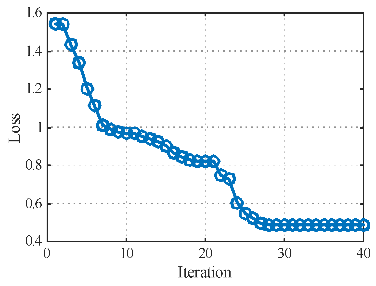
The structure of the intermediate-stage flux temperature prediction model is set as a two-layer GRU network and a one-layer fully connected network. The maximum epochs of the training process are set to 20, and the learning rate is initially set to 0.01. The learning rate decay strategy is adopted, with the learning rate decaying by 0.5 every five batches, and the Minibatch size is set to 1024. The initial settings of the model’s GRU neurons are 120 and 60, at which time the training time is 196 s, and the RMSE of the training is 0.5014. The number of GRU model neurons is selected as the optimization parameter, the training RMSE is the objective function, and the maximum number of iterations is 40. The optimization ranges of the first and second GRU layers of neurons are (60, 120) and (20, 60), respectively. The actual optimization process is shown in Figure 8.
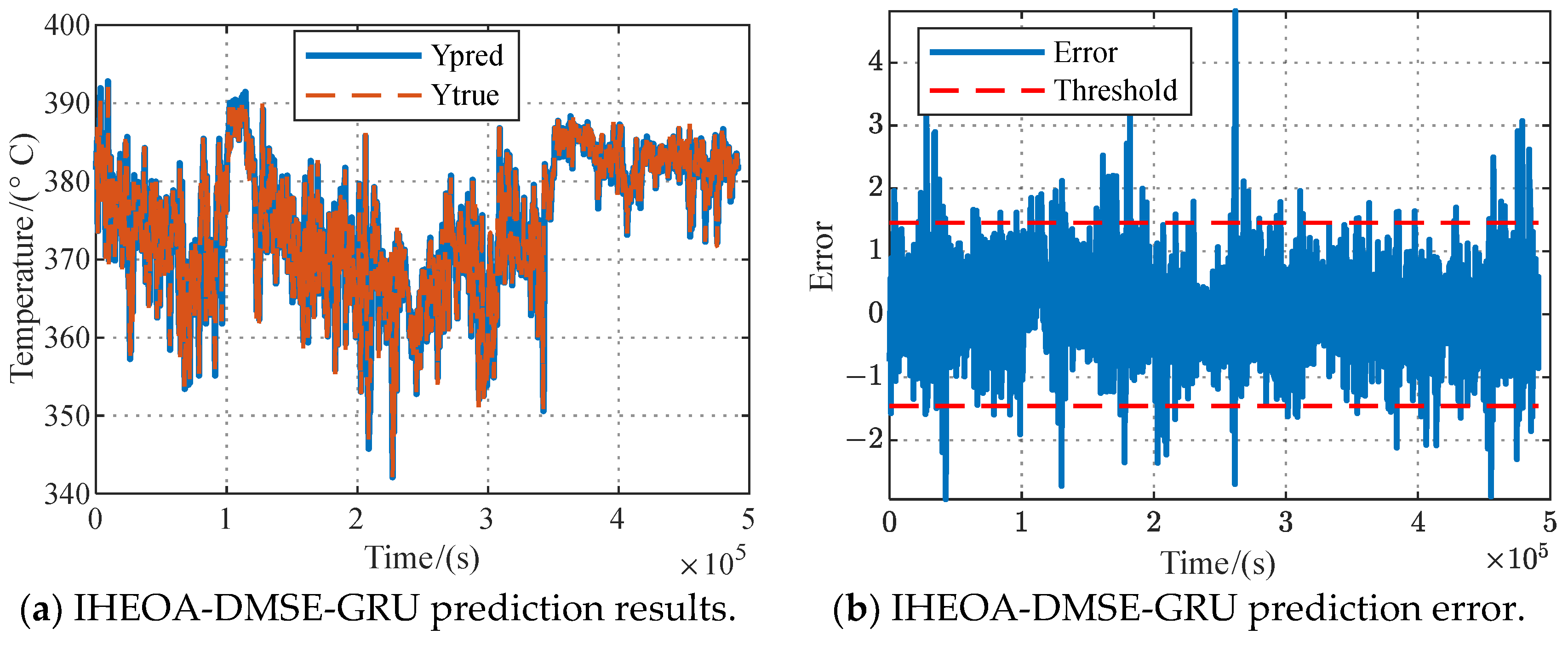
Figure 8 shows that the proposed IHEOA algorithm has faster convergence in the GRU optimization process. Meanwhile, the prediction error decreases again at 20 iterations, indicating that the proposed algorithm has the ability to break through the local optimum. The final number of GRU neurons in two layers is 89 and 58. The training time with this set of parameters is 190 s, and the training RMSE is 0.4866. Compared with the initial model, the training time and training accuracy are improved by 3.06% and 2.95%. The model prediction of the training data is shown in Figure 9a. The prediction error is shown in Figure 9b.
From Figure 9, it can be seen that the prediction error is normally distributed, which satisfies the conditions of the long-mode fault warning model. The error sig is calculated to be 0.4581, so the threshold value of the first intermediate-stage flux fault warning is [−1.455, 1.455]. The model trained under this parameter is saved for subsequent fault diagnosis experiments.
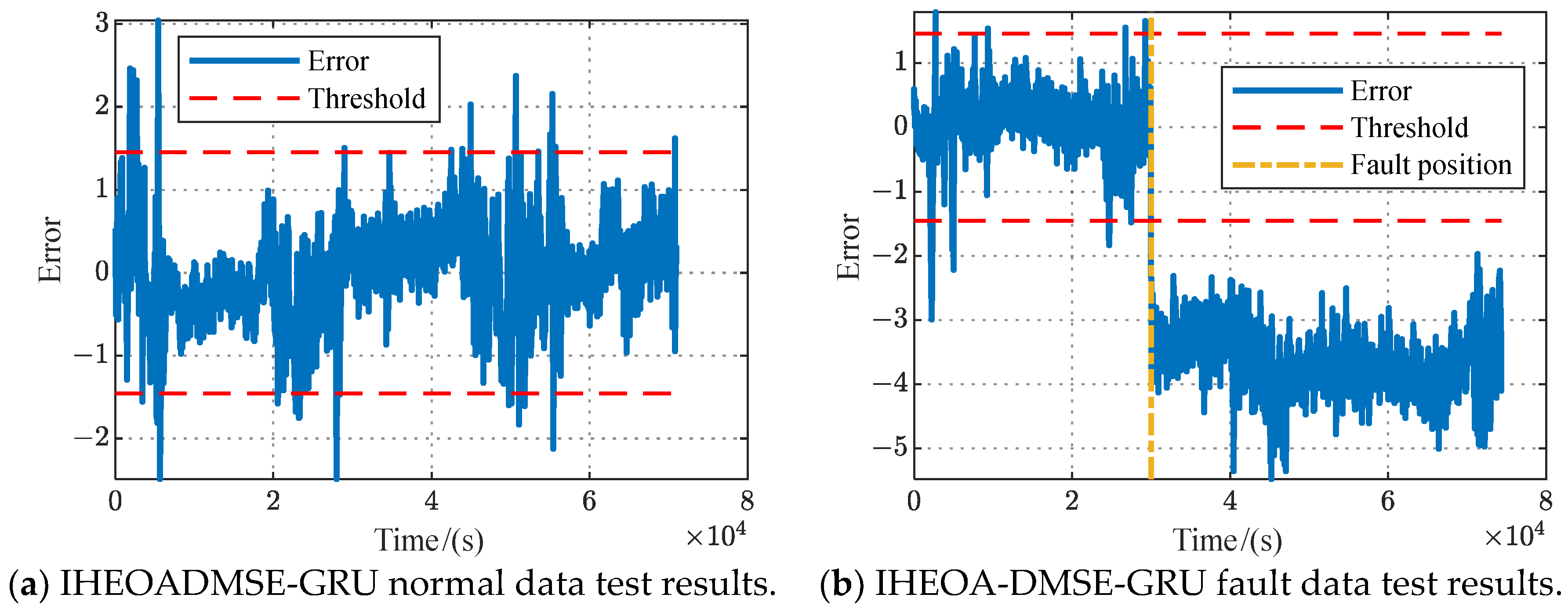
The model was tested using both test data. The model prediction errors of temperature after the stage under normal and fault data are shown in Figure 10a,b. The diagnostic accuracies are 0.9902 and 1.000, respectively, and the false alarm rate is only 0.0098, which is able to sensitively identify the steam turbine intermediate-stage flux operation health status.

4. Comparative Experimental Results

4.1. Results without IHEOA Optimization

In order to highlight the role of the IHEOA optimization algorithm for early and sensitive fault warning, the test data are tested using the normal DMSE-GRU model with two layers of 120 and 60 hidden nodes. The test results are shown in Figure 11.
The diagnostic accuracy of the normal DMSE-GRU model in the two test data is 0.9684 and 0.9986, respectively. Compared with the IHEOA optimized model, the diagnostic accuracy is reduced by 2.18% and 0.14%, respectively. The false alarm rate is increased by 2.22 times. This reflects the necessity and superiority of the algorithm proposed in this study.
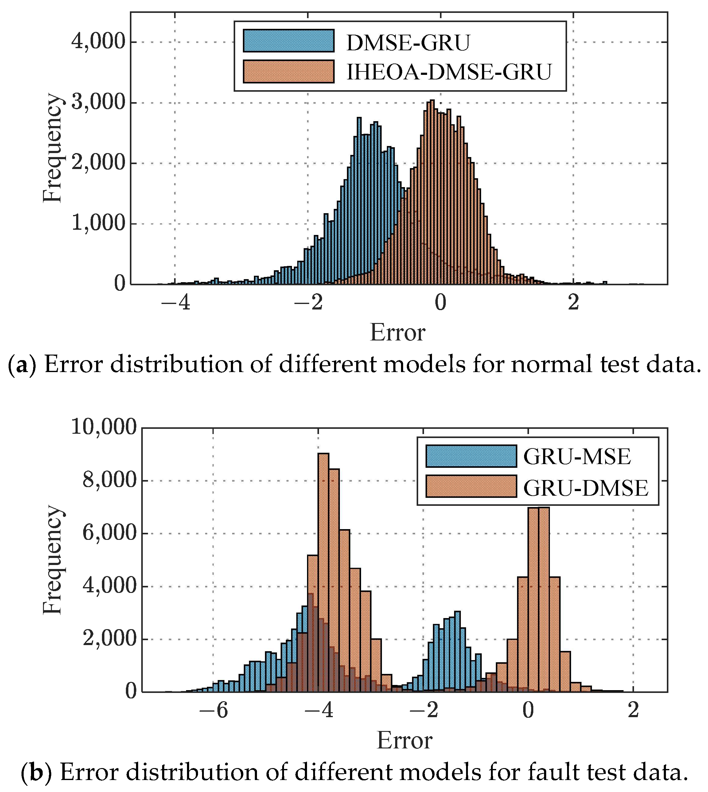
The distribution of prediction errors of the model on the test set before and after optimization are shown in Figure 12a,b.
It can be clearly seen from Figure 12 that the prediction error of the proposed method satisfies the normal distribution, and the frequency of error is 0. There is almost no overlap between the errors of fault data and normal data. The proposed method has the smallest intra-class distance and the largest class spacing. This indicates that the proposed method is more suitable for the early warning of turbine-stage group flux faults. While the direct use of the GRU model can achieve a certain degree of fault detection, it is difficult to be put into practical application due to the high overlap of different classes with a high false alarm rate.

4.2. Comparison Results for Different Loss Functions

The proposed DMSE loss function and the traditional MSE loss function are used to train and test the GRU model. Some of the test data prediction results are shown in Figure 13. It can be seen that the prediction results of the proposed DMSE loss function can more closely match the actual temperature trend.
The dynamic change in temperature after the steam turbine intermediate flow stage has a certain time correlation. The DMSE loss function proposed in this paper not only focuses on the prediction error, but also focuses on the shape matching of the prediction results, which can obtain the prediction value that is more in line with the actual dynamic change process. Fault warning experiments are carried out using the GRU-MSE model. The diagnostic accuracies of normal and fault test data are 0.9506 and 0.9890, respectively. Compared with the ordinary GRU model, the proposed method improves the diagnostic accuracy in normal and fault data by 3.96% and 1.10%, respectively.

4.3. Comparison Results with Traditional Model

In order to highlight the superiority of the proposed method, multiple temperature prediction models are trained using the traditional methods and the same training data. Fault diagnosis experiments are carried out using the test data and the resulting model. The diagnostic accuracies of the different methods are shown below in Table 1. Comparison algorithms include LSTM, convolutional neural network (CNN), BP, extreme learning machines (ELMs), gradient boosting decision tree (GBDT), and LightGBM.
It can be seen from Table 1 that the proposed method obtains the highest diagnostic accuracy with optimal performance on normal and fault data. The proposed method improves the diagnostic accuracy by an average of 1.31% with normal data and reduces the false alarm rate by an average of 1.03% in case of failure. This is due to the fact that the IHEOA is highly efficient in optimizing the parameters, while the DMSE loss function improves the accuracy of the training process.

5. Conclusions

In the energy background of high-proportion penetration of wind and new energy sources, thermal power units play an increasingly important regulating role. Therefore, the safety of thermal power units has received more and more attention. As the most critical work unit of the turbine, the operation stability of the intermediate-stage flux affects the work and regulation capability of the turbine. Due to the frequent and wide-ranging variable operating conditions of thermal power units, the working environment of the intermediate-stage group becomes more and more severe, and the probability of performance degradation increases. It is necessary to carry out the sensitive identification of its early failure warning. Aiming at this problem, this paper proposes a DMSE-GRU constant-mode fault early warning model and uses IHEOA to optimize the model parameters. The following conclusions can be drawn from experiments with actual thermal power unit operating data.
(1)
The HEOA algorithm is improved by introducing lens opposition-based learning, so that it obtains a more powerful parameter optimization capability. The optimization results have a low-cost function value and the fastest optimization speed compared with the traditional HEOA, GWO, WOA, and SSA optimization algorithms. Also, the diagnostic accuracy can be improved by 2.18% and 0.14% compared to the unoptimized model.
(2)
The proposed DMSE-GRU model is able to obtain prediction results that are more in line with the actual change trend by introducing shape similarity and error minimization as the loss function objectives. Compared with the GRU model, the proposed method improves the diagnostic accuracy in normal and fault data by 3.96% and 1.10%, respectively.
(3)
The proposed IHEOA-DMSE-GRU model achieves the highest diagnostic accuracy. The detection accuracy of normal and fault data reaches 99.02% and 100%, respectively. Compared to the conventional six neural networks, the proposed method improved the detection accuracy by an average of 1.31% and 1.03% under normal and faulty conditions.
By establishing a high-precision temperature prediction model, the proposed method can effectively improve the fault early warning accuracy, significantly improve the thermal power unit operation safety, and thus guarantee the stability of power grid operation. In the future, we will extend the proposed optimization algorithm and loss function to more complex prediction models.

Author Contributions

Conceptualization, M.C.; methodology, M.C.; software, M.C.; validation, Q.Z. and Y.C.; formal analysis, Q.Z.; investigation, Q.Z.; resources, Y.C.; data curation, Y.C.; writing—original draft preparation, M.C.; writing—review and editing, M.C. and Q.Z.; visualization, Y.C.; funding acquisition, M.C., Q.Z. and Y.C. All authors have read and agreed to the published version of the manuscript.

Funding

This research received no external funding.

Data Availability Statement

Data available on request due to device privacy restrictions.

Conflicts of Interest

Author Ming Cheng was employed by the company State Power Investment Inner Mongolia Energy Co., Ltd. and Author Qiang Zhang was employed by the company Shanghai Power Equipment Research Institute Co., Ltd. The remaining authors declare that the research was conducted in the absence of any commercial or financial relationships that could be construed as a potential conflict of interest.

Nomenclature

Abbreviations
HEOAhuman evolutionary optimization
IHEOAimproved HEOA algorithm
L1lasso regression
BPback propagation
LSTMlong short-term memory
MSEmean squared error
CNNconvolutional neural network
ANNsartificial neural networks
RNNsrecurrent neural networks
GRUgate recurrent unit
PSOparticle swarm optimization
GWOgrey wolf optimization
DTWdynamic time warping
DMSEdynamic time warping and mean squared error
WOAwhale optimization algorithm
SSAsalp swarm algorithm
ELMsextreme learning machines
GBDTgradient boosting decision tree
Subscripts/superscript
t time
i location of data
f fully connected network
r reset gate
h cell state
z update gate
i t e r number of search iterations
m e a n average position
b e s t best position
*reverse point
k number of paths
m signal length
n signal length
Symbols
Y performance characterization parameters
F equipment state functions
X measurement parameters
θ structural parameters
h cell state
x input sensor data
W weight matrices
r reset factor
tanh hyperbolic tangent function
h ˜ candidate cell state
z update factor
Y ^ forecast performance parameters
dim data dimension
f l o o r rounding downwards
L e v y levy distribution
j u m p jump coefficient
r a n d n random number in [0, 1]
o n e s ( 1 , d i m ) row vector in column dim
R n complexity factor
A evaluation value
o base point
a maximum boundaries
b minimum boundaries
k scale factor
N sample size
y ^ predicted value
y true value
d Euclidean distance
w matrix paths
min minimum function
ω knowledge acquisition ease coefficient
σ sigmoid function

References

  1. Bai, M.; Liu, J.; Chai, J.; Zhao, X.; Yu, D. Anomaly detection of gas turbines based on normal pattern extraction. Appl. Therm. Eng. 2020, 166, 114664. [Google Scholar] [CrossRef]
  2. Gonzalez-Salazar, M.A.; Kirsten, T.; Prchlik, L. Review of the operational flexibility and emissions of gas- and coal-fired power plants in a future with growing renewables. Renew. Sustain. Energy Rev. 2018, 82, 1497–1513. [Google Scholar] [CrossRef]
  3. Lee, J.J.; Kang, S.Y.; Kim, T.S.; Park, S.J.; Hong, G.W. The effect of hub leakage on the aerodynamic performance of high-pressure steam turbine stages. J. Mech. Sci. Technol. 2017, 31, 445–454. [Google Scholar] [CrossRef]
  4. Goyal, V.; Xu, M.; Kapat, J.; Vesely, L. Prediction Enhancement of Machine Learning Using Time Series Modeling in Gas Turbines. J. Eng. Gas Turbines Power 2023, 145, 121005. [Google Scholar] [CrossRef]
  5. Hu, P.; Cao, L.; Su, J.; Li, Q.; Li, Y. Distribution characteristics of salt-out particles in steam turbine stage. Energy 2020, 192, 116626. [Google Scholar] [CrossRef]
  6. Jia, K.; Liu, C.; Li, S.; Jiang, D. Modeling and optimization of a hybrid renewable energy system integrated with gas turbine and energy storage. Energy Convers. Manag. 2023, 279, 116763. [Google Scholar] [CrossRef]
  7. Gong, L.; Hou, G.; Li, J.; Gao, H.; Gao, L.; Wang, L.; Gao, Y.; Zhou, J.; Wang, M. Intelligent fuzzy modeling of heavy-duty gas turbine for smart power generation. Energy 2023, 277, 127641. [Google Scholar] [CrossRef]
  8. Guandalini, G.; Campanari, S.; Romano, M.C. Power-to-gas plants and gas turbines for improved wind energy dispatchability: Energy and economic assessment. Appl. Energy 2015, 147, 117–130. [Google Scholar] [CrossRef]
  9. Tahan, M.; Tsoutsanis, E.; Muhammad, M.; Karim, Z.A. Performance-based health monitoring, diagnostics and prognostics for condition-based maintenance of gas turbines: A review. Appl. Energy 2017, 198, 122–144. [Google Scholar] [CrossRef]
  10. Salahshoor, K.; Kordestani, M.; Khoshro, M.S. Fault detection and diagnosis of an industrial steam turbine using fusion of SVM (support vector machine) and ANFIS (adaptive neuro-fuzzy inference system) classifiers. Energy 2010, 35, 5472–5482. [Google Scholar] [CrossRef]
  11. Hashmi, M.B.; Mansouri, M.; Fentaye, A.D.; Ahsan, S.; Kyprianidis, K. An Artificial Neural Network-Based Fault Diagnostics Approach for Hydrogen-Fueled Micro Gas Turbines. Energies 2024, 17, 719. [Google Scholar] [CrossRef]
  12. Li, X.; Chang, H.; Wei, R.; Huang, S.; Chen, S.; He, Z.; Ouyang, D. Online Prediction of Electric Vehicle Battery Failure Using LSTM Network. Energies 2023, 16, 4733. [Google Scholar] [CrossRef]
  13. Li, X.; Liu, J.; Bai, M.; Li, J.; Li, X.; Yan, P.; Yu, D. An LSTM based method for stage performance degradation early warning with consideration of time-series information. Energy 2021, 226, 120398. [Google Scholar] [CrossRef]
  14. Yang, Z.; Qiao, L.; Su, M.; Hu, Z.; Teng, X.; Wang, J. Ionospheric foF2 nowcast based on a machine learning GWO-ALSTM model. Adv. Space Res. 2023, 72, 4896–4910. [Google Scholar] [CrossRef]
  15. Bharti, P.; Redhu, P.; Kumar, K. Short-term traffic flow prediction based on optimized deep learning neural network: PSO-Bi-LSTM. Phys. A Stat. Mech. Its Appl. 2023, 625, 129001. [Google Scholar] [CrossRef]
  16. Lu, P.; Ye, L.; Zhong, W.; Qu, Y.; Zhai, B.; Tang, Y.; Zhao, Y. A novel spatio-temporal wind power forecasting framework based on multi-output support vector machine and optimization strategy. J. Clean. Prod. 2020, 254, 119993. [Google Scholar] [CrossRef]
  17. Priya, G.V.; Ganguly, S. Multi-swarm surrogate model assisted PSO algorithm to minimize distribution network energy losses. Appl. Soft Comput. 2024, 159, 111616. [Google Scholar] [CrossRef]
  18. Phan, Q.B.; Nguyen, T.T. Enhancing wind speed forecasting accuracy using a GWO-nested CEEMDAN-CNN-BiLSTM model. ICT Express 2023, 10, 485–490. [Google Scholar] [CrossRef]
  19. Olayode, I.O.; Tartibu, L.K.; Okwu, M.O.; Severino, A. Comparative Traffic Flow Prediction of a Heuristic ANN Model and a Hybrid ANN-PSO Model in the Traffic Flow Modelling of Vehicles at a Four-Way Signalized Road Intersection. Sustainability 2021, 13, 10704. [Google Scholar] [CrossRef]
  20. Houran, M.A.; Bukhari, S.M.S.; Zafar, M.H.; Mansoor, M.; Chen, W. COA-CNN-LSTM: Coati optimization algorithm-based hybrid deep learning model for PV/wind power forecasting in smart grid applications. Appl. Energy 2023, 349, 121638. [Google Scholar] [CrossRef]
  21. Hu, Q.; Zhou, N.; Chen, H.; Weng, S. Bayesian damage identification of an unsymmetrical frame structure with an improved PSO algorithm. Structures 2023, 57, 105119. [Google Scholar] [CrossRef]
  22. Li, F.; Li, Y. Robust echo state network with Cauchy loss function and hybrid regularization for noisy time series prediction. Appl. Soft Comput. 2023, 146, 110640. [Google Scholar] [CrossRef]
  23. He, X.; Tan, S.; Wu, Z.; Zhang, L. Mission reconstruction for launch vehicles under thrust drop faults based on deep neural networks with asymmetric loss functions. Aerosp. Sci. Technol. 2022, 121, 107375. [Google Scholar] [CrossRef]
  24. Zhou, Z.; Zhang, W.; Yao, P.; Long, Z.; Bai, M.; Liu, J.; Yu, D. More realistic degradation trend prediction for gas turbine based on factor analysis and multiple penalty mechanism loss function. Reliab. Eng. Syst. Saf. 2024, 247, 110097. [Google Scholar] [CrossRef]
  25. Sharma, A.; Sundaram, S. An enhanced contextual DTW based system for online signature verification using Vector Quantization. Pattern Recognit. Lett. 2016, 84, 22–28. [Google Scholar] [CrossRef]
  26. Iwana, B.K.; Frinken, V.; Uchida, S. DTW-NN: A novel neural network for time series recognition using dynamic alignment between inputs and weights. Knowl.-Based Syst. 2020, 188, 104971. [Google Scholar] [CrossRef]
  27. Muscillo, R.; Schmid, M.; Conforto, S.; D’Alessio, T. Early recognition of upper limb motor tasks through accelerometers: Real-time implementation of a DTW-based algorithm. Comput. Biol. Med. 2011, 41, 164–172. [Google Scholar] [CrossRef] [PubMed]
  28. Li, Q.; Zhang, X.; Ma, T.; Liu, D.; Wang, H.; Hu, W. A Multi-step ahead photovoltaic power forecasting model based on TimeGAN, Soft DTW-based K-medoids clustering, and a CNN-GRU hybrid neural network. Energy Rep. 2022, 8, 10346–10362. [Google Scholar] [CrossRef]
  29. Zhou, Z.; Bai, M.; Long, Z.; Liu, J.; Yu, D. An adaptive remaining useful life prediction model for aeroengine based on multi-angle similarity. Measurement 2024, 226, 114082. [Google Scholar] [CrossRef]
  30. Tang, J.; Liu, C.; Yang, D.; Ding, M. Prediction of ionospheric TEC using a GRU mechanism method. Adv. Space Res. 2024, 74, 260–270. [Google Scholar] [CrossRef]
  31. Lian, J.; Hui, G. Human Evolutionary Optimization Algorithm. Expert Syst. Appl. 2024, 241, 122638. [Google Scholar] [CrossRef]
  32. Kaidi, W.; Khishe, M.; Mohammadi, M. Dynamic Levy Flight Chimp Optimization. Knowl.-Based Syst. 2022, 235, 107625. [Google Scholar] [CrossRef]
  33. Wu, D.; Rao, H.; Wen, C.; Jia, H.; Liu, Q.; Abualigah, L. Modified Sand Cat Swarm Optimization Algorithm for Solving Constrained Engineering Optimization Problems. Mathematics 2022, 10, 4350. [Google Scholar] [CrossRef]
  34. Yao, X.; Liu, Y.; Lin, G. Evolutionary programming made faster. IEEE Trans. Evol. Comput. 1999, 3, 82–102. [Google Scholar] [CrossRef]
  35. Elsisi, M. Optimal design of adaptive model predictive control based on improved GWO for autonomous vehicle considering system vision uncertainty. Appl. Soft Comput. 2024, 158, 111581. [Google Scholar] [CrossRef]
  36. Song, Y.; Xie, H.; Zhu, Z.; Ji, R. Predicting energy consumption of chiller plant using WOA-BiLSTM hybrid prediction model: A case study for a hospital building. Energy Build. 2023, 300, 113642. [Google Scholar] [CrossRef]
  37. Mirjalili, S.; Gandomi, A.H.; Mirjalili, S.Z.; Saremi, S.; Faris, H.; Mirjalili, S.M. Salp Swarm Algorithm: A bio-inspired optimizer for engineering design problems. Adv. Eng. Softw. 2017, 114, 163–191. [Google Scholar] [CrossRef]
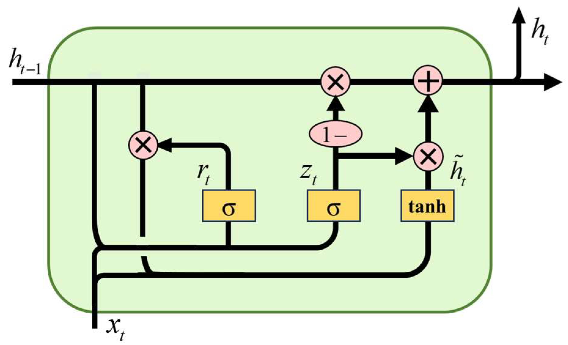
Figure 1. Illustration of GRU structure.
Energies 17 03629 g001
Figure 2. Lens opposition-based learning diagram.
Energies 17 03629 g002
Figure 3. Flowchart of IHEOA algorithm.
Energies 17 03629 g003
Figure 4. DTW calculation process.
Energies 17 03629 g004
Figure 5. Proposed methodological framework.
Energies 17 03629 g005
Figure 6. Division of experimental data.
Energies 17 03629 g006
Figure 7. Optimization results of different optimization algorithms.
Energies 17 03629 g007
Figure 8. IHEOA model optimization process.
Energies 17 03629 g008
Figure 9. IHEOA-DMSE-GRU model training results.
Energies 17 03629 g009
Figure 10. Test results of IHEOA-DMSE-GRU model.
Energies 17 03629 g010
Figure 11. Test results of DMSE-GRU model.
Energies 17 03629 g011
Figure 12. Error distribution of different models.
Energies 17 03629 g012
Figure 13. Comparison of different loss functions.
Energies 17 03629 g013
Table 1. Comparison of diagnostic accuracy of different models.
ModelNormal Test SetImprovementFaulty Test SetImprovement
Proposed method0.9902/1.000/
LSTM0.96542.57%0.99980.02%
CNN0.97561.50%0.99880.12%
BP0.96532.58%0.98711.31%
ELM0.98021.02%0.98012.03%
GBDT0.98900.12%0.98411.62%
LightGBM0.98920.10%0.98931.08%
Disclaimer/Publisher’s Note: The statements, opinions and data contained in all publications are solely those of the individual author(s) and contributor(s) and not of MDPI and/or the editor(s). MDPI and/or the editor(s) disclaim responsibility for any injury to people or property resulting from any ideas, methods, instructions or products referred to in the content.