1. Introduction
Microgrids refer to a distributed network of loads and energy generation units confined within specific electrical boundaries and can be categorized into two main groups: AC and DC. DC microgrids offer several advantages over AC ones, including higher efficiency, lower cost, simplified control, protection, and smaller system size [
1,
2]. DC–DC power electronic converters play an important role in microgrid control and operation by facilitating efficient power transfer between different components of a microgrid by converting DC from one voltage level to another [
3,
4]. They are widely used in various applications such as industrial automation, aerospace, renewable energy systems, electric cars, fast EV DC chargers, and interfaces between DC catenaries and DC loads.
In these applications, it is necessary not only to optimize the temporal response but also to optimize the efficiency and nonlinear behavior of the converter. Therefore, it is essential to apply advanced control techniques such as DRL-based controllers. Moreover, these converters can operate in different modes, such as buck or boost converters that can function in DCM, CCM, or DAB converters that have multiple modulation techniques. This flexibility allows for managing different load conditions and improving performance across various applications. Among the various categories of DC–DC power electronic converters, the buck converter stands out as a popular choice due to its simplicity and high efficiency.
Numerous research studies have investigated control methods for DC–DC power electronic converters, including classical design methods such as proportional–integral–derivative (PID) control [
5], nonlinear techniques like sliding mode control (SMC) [
6,
7], model predictive control (MPC) [
8,
9], etc. Although these control methods perform well, they often rely on detailed system models. The design process of these control methods is typically based on the converter’s average model, which captures only the average behavior of the converters and does not consider the switching model. For instance, in the case of dual active bridge (DAB) converters, achieving precise control and ensuring effectiveness requires consideration of the switching model, especially when integrating modulations that vary depending on the operating points [
10]. Moreover, it is challenging to achieve fast and accurate control performance due to the different factors such as parameter uncertainties, nonlinearities, input voltage disturbances, and time-varying operational scenarios in complex power converter topologies.
Recent advancements in passivity-based control have shown significant improvements in the performance of power electronic systems [
11]. Additionally, model-free intelligent controllers such as neural networks and fuzzy logic controllers [
12,
13,
14] have been developed without requiring an explicit model of the system. Notably, the study of [
15] demonstrates the effectiveness of a fuzzy logic controller in mitigating harmonics and managing reactive power in three-level shunt active filters. These controllers are suitable for specific time intervals; however, they often lack the capability for online learning.
With the rapid advancement in machine learning, DRL-based techniques, which encompass both model-based and model-free approaches, have captured significant attention and demonstrated remarkable success in addressing complex and nonlinear behaviors across various intricate problems due to their self-learning characteristics. Model-free DRL methodologies, such as the PPO algorithm, do not require a detailed mathematical model of the system they control. Instead, they learn optimal policies directly from interactions with the environment, making decisions based on trial and error to maximize cumulative rewards. This can be applied in designing complex controllers with novel functionalities for power electronic converters, particularly in scenarios where obtaining results with traditional control techniques may not be straightforward. DRL enables adaptation to converters’ switching models across the entire operating range and their variations at different operating points.
Unlike traditional methods, these DRL-based methods can be used to control different configurations of DC–DC power electronic converters, including boost, buck-boost, DAB, and cascaded H-bridge (CHB) converters, simply by retraining the agents in new environments. In [
16], a DRL-based optimization algorithm is proposed for optimizing the design parameters of power electronic converters using a deep neural network (DNN)-based surrogate model. It is important to note that by considering the same fundamentals of the DRL design, such as the neural network structure, reward function, training hyperparameters, and other details of the DRL methodology, the proposed method can be extended to other topologies of converters. This can be carried out by changing the environment in the Simulink model and then retraining the agent for the new environment.
In theses state-of-the-art studies, there are some works that have focused on employing DRL-based controllers for voltage control in DC–DC power electronic converters. For example, the deep deterministic policy gradient (DDPG) algorithm is utilized in [
17], enabling effective control of the output voltage of the buck converter for precise tracking of a reference voltage in dynamic environments. In the study [
18], the deep Q-network (DQN) algorithm is implemented for an intelligent adaptive model predictive controller, demonstrating the ability to optimize control actions considering the converter’s states and environmental conditions. This method is applied to a DC–DC buck-boost converter in the presence of significant CPL variations. Ref. [
19] investigates the voltage control of a buck converter using two RL agents, namely DQN and DDPG, benchmarked against controllers such as SMC and MPC. Another research suggests a PPO-based ultra-local model (ULM) scheme for achieving voltage stabilization in DC–DC buck-boost converters feeding constant power loads (CPLs) [
20]. The primary focus of the work [
21] is on the development of an online training artificial intelligence (AI) controller for DC–DC converters employing the DDPG algorithm. The controller is applicable to all types of DC–DC converters and can address a variety of control objectives. In [
22], an RL regression-based voltage regulator for boost converters is proposed, integrating the PWM technique. It is a model-based method requiring an accurate average model of the converter and a suitable set of kernel functions. Furthermore, in [
23], an intelligent PI controller coupled with an RL-based auxiliary controller is discussed to stabilize the output voltage of a buck converter under CPL conditions. This approach is also model-based and involves manipulation of the duty cycle of the PWM signal. In [
24], a novel algorithm utilizing DQN is introduced for parameter optimization, aiming to improve the design of power electronic converters. Moreover, a new online integral reinforcement learning (IRL)-based data-driven control algorithm for the interleaved DC–DC boost converter is proposed in [
25]. Additionally, [
26] demonstrates a variable-frequency triple-phase-shift (TPS) control strategy employing deep reinforcement learning to enhance the conversion efficiency of the dual-active-bridge converter. The ANN-RL (artificial neural networks-reinforcement learning) approach is employed in [
27,
28] to regulate the operation of the buck converter, showing robustness against parameter variations and load changes.
Although different DRL algorithms are proposed for power electronic converters in these state-of-the-art studies, some gaps remain in the body of knowledge regarding the impact of neural network structure on control performance and computational efficiency. Additionally, these studies do not explore the use of different input features to improve decision-making. They also lack guidelines for choosing training hyperparameters, network size, and reward function. These studies typically use an average model of the power electronic converter, which simplifies the converter’s dynamics. In contrast, the proposed method in this work uses a detailed switching model that captures the complex behavior of the converter more accurately. Moreover, the performance of DC–DC power electronic converters in these studies is not considered in both modes of operations (DCM and CCM) and usually focuses on one type of load. Furthermore, the behavior of changing integral gain in the input of ANNs is also rarely studied.
Therefore, a study on the DRL training process using a switching model of DC–DC power electronic converters in different modes of operation with varying loads, along with an easily implemented DRL in real life that considers memory consumption, could be very useful. This study is not intended to perform a comparison between conventional methods and DRL controllers, as this has already been done in several studies such as [
19,
23,
29]. These studies have shown that DRL-based controllers can control power electronic converters better than traditional controllers in complex scenarios. The main objective of this paper is to explore the potential and capabilities of model-free DRL-based controllers, particularly the PPO agent, in the control of DC–DC power electronic converters. This approach addresses existing gaps by providing a comprehensive method for enhancing control and optimization.
Our key contributions include the following:
Proposing a complete training guide for DRL agents to control real power electronic converters in different modes of operation using a detailed switching model that considers real-life delays. This guide also takes into account the introduction of a chattering-reduction term in the reward function and input feature selection and evaluates the impact of network size.
Analyzing the trade-off between neural network configuration, computational efficiency, memory usage, and control performance accuracy through experimental tests.
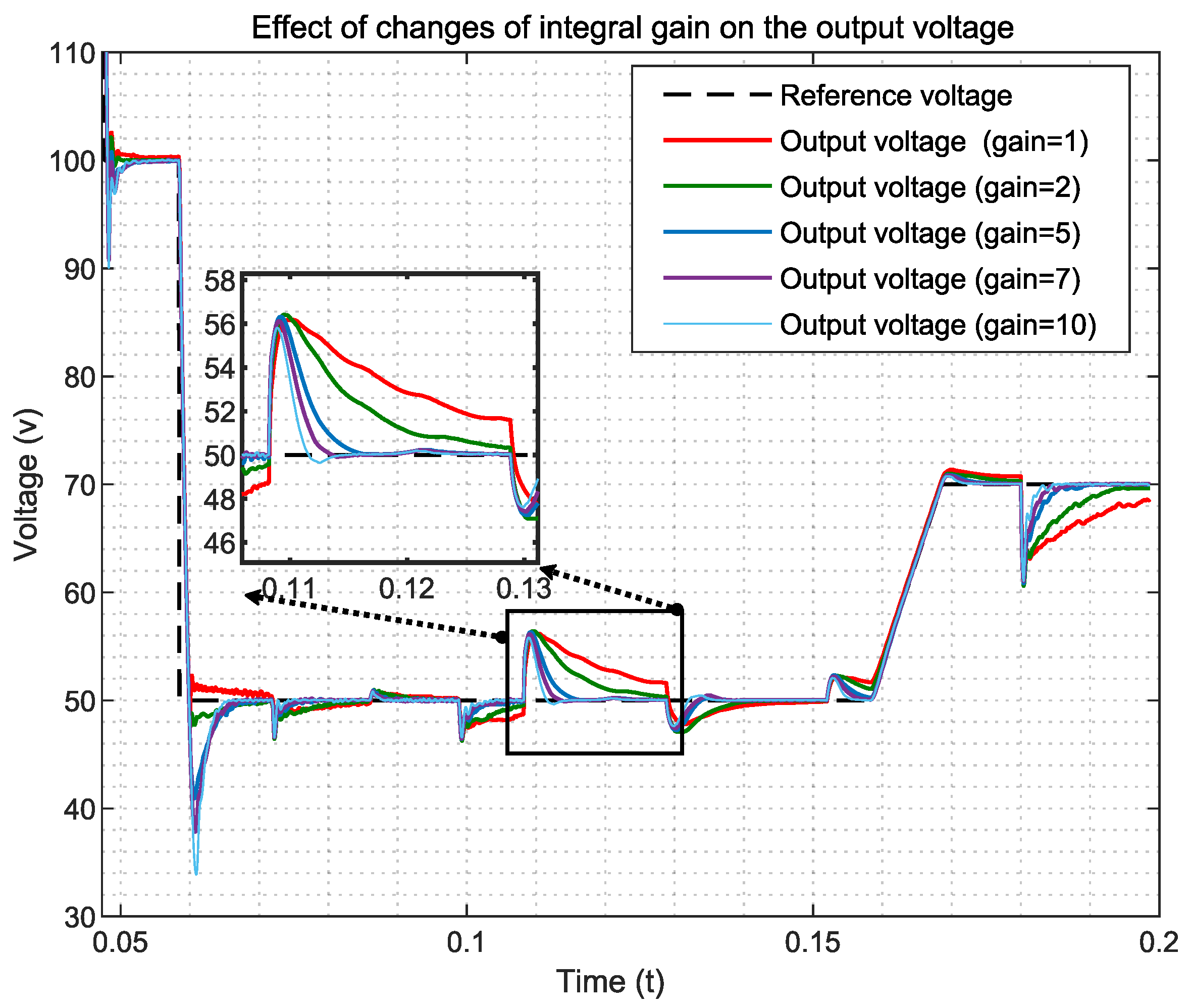
Adding an adjustable gain in the integral error input, allowing control over transient responses without the need to retrain the DRL agent.
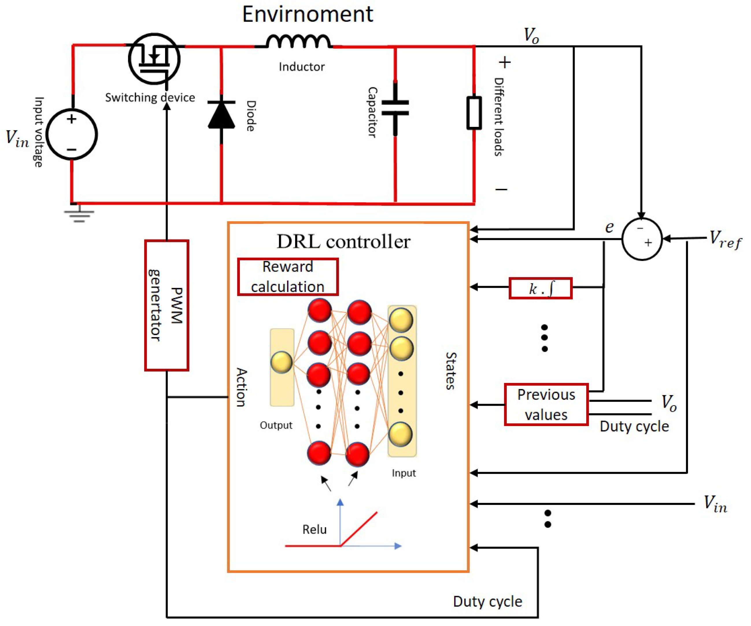
The general control scheme of the proposed DRL controller for a buck converter is presented in
Figure 1.
The rest of this paper is organized as follows. The next section provides a brief introduction to the fundamental principles of the DRL approach and the structure of the PPO algorithm. Following that, a practical case study for the buck converter is explored, implementing the DRL algorithm. The paper then presents the simulation and experimental results of the proposed algorithm in various scenarios. Finally, the conclusions drawn from the study are discussed.
2. DRL-Based Controller-Choosing Guide
DRL algorithms [
30] can be broadly categorized as either model-based or model-free, as illustrated in
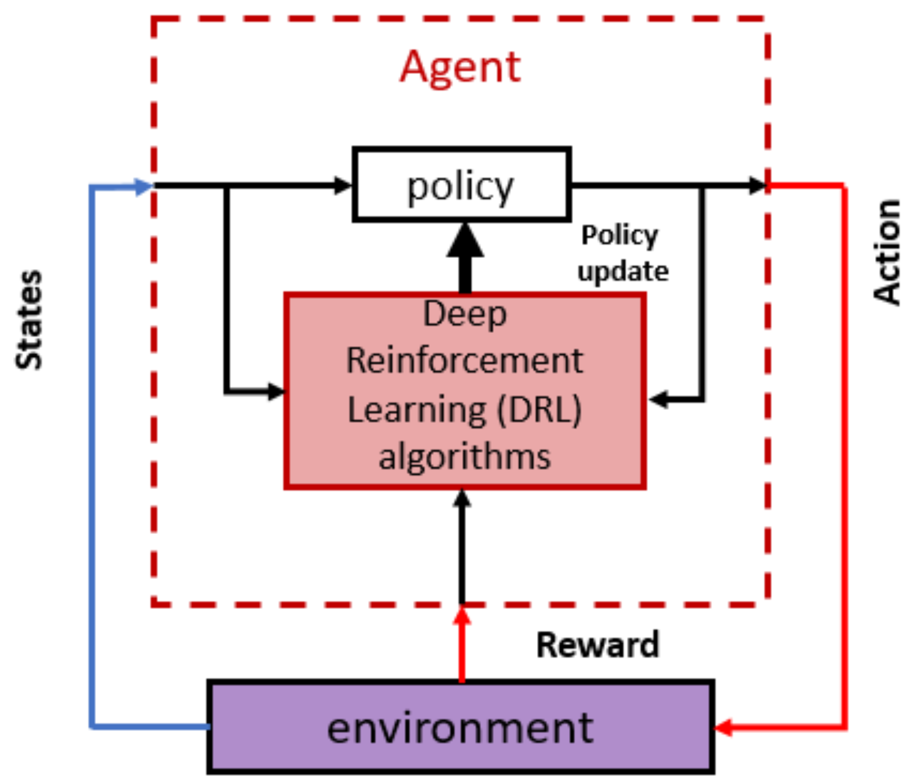
Table 1, in which ✓✓, ✓, and - present High, Medium, and Low or None respectively. Recently, there has been a growing interest in model-free algorithms which focus on training agents to learn a near-optimal policy through iterative interactions with an environment, as shown in
Figure 2. This involves receiving feedback in the form of rewards and adjusting neural network parameters to maximize cumulative discounted rewards over time, as defined in Equation (
1) [
30], where
is the discount factor applied to future rewards,
is the policy, and
is the reward at time step
t.
A DRL environment is formally defined as a Markov decision process (MDP). The MDP framework outlines decision-making under the Markovian assumption, where the next state of the environment is solely influenced by the current state and the agent’s action within it. An MDP is denoted as a tuple
, where
S and
A represent the state and action space, respectively. The transition matrix
determines the probability of transitioning from one state to another when performing an action. Additionally, the matrix
specifies the reward of each transition [
30]. In the following, each of them is described in detail.
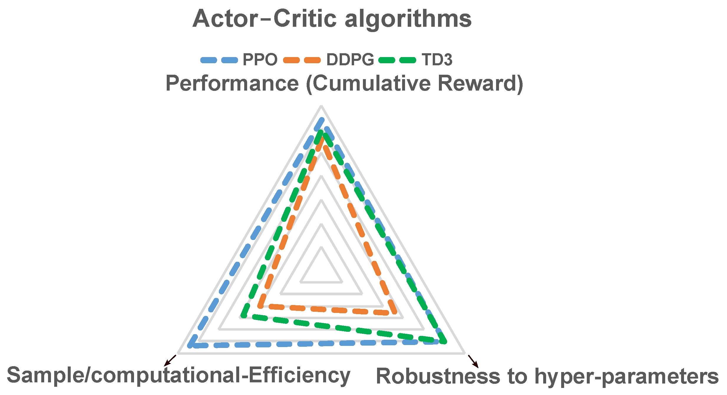
Among various model-free DRL algorithms, an actor–critic structure synergistically combines the strengths of both policy-based and value-based methods, enhancing the stability and efficiency of learning. This architecture consists of two essential components: an actor selects actions based on the current state of the environment, while a critic is typically responsible for evaluating actions and providing feedback on their effectiveness so as to achieve the desired goals. The critic is defined by another neural network.
Figure 3 illustrates the rationality behind the choice of PPO as an actor–critic algorithm for controlling DC–DC power electronic converters. This choice is based on its stability, sample/computational efficiency, ability to perform online policy updates, continuous adaptation to evolving or diverse environments, and ease of implementation [
31,
32]. Consequently, these features make the PPO a suitable candidate for real-time control applications [
33]. The PPO and its variant, PPO-Clipped [
34], focus on minimizing excessive policy updates at each step, leading to a more stable training procedure.
2.1. Fundamentals of the Design
In the design of DRL controllers for power electronic converters, it is crucial to carefully consider several fundamental aspects. These include the definition of the state space and input feature selection, action space, reward function engineering, and the architecture of the neural network. Each of these elements plays an important role in ensuring that the DRL agent can learn effectively and perform robustly when controlling the power converter.
2.1.1. State Space
The state, which contains a set of features, must contain adequate information to comprehensively describe the system environment. Hence, the selection of relevant states is vital in the design of a DRL system to improve the learning process. Apart from existing studies, additional features are considered to enable more informative decisions, representing the input information the agent receives from the environment at each time step
t. Due to the consideration of various objectives and scenarios, the features encompass all time-changing variables and context parameters (refer to time-independent features), thereby enhancing the system’s capabilities [
35]. Remarkably, there is a trade-off between the number of previous feature values (
) used in the states, the training time, and the size of the network. Larger values of
lead to more efficient decisions, although this entails increased complexity. Based on extensive simulation results, this study determines that 4 is the most suitable number of previous values, reflecting a balance between effective learning and computational efficiency.
Table 2 shows the feature vector
, where
,
,
,
,
k,
, and
represent the output voltage, voltage tracking error, duty cycle, input voltage, integral gain, reference voltage, and maximum output voltage, respectively.
serves as a constant for normalization. The feature vector has 19 components. Moreover, all values of the feature vector are normalized using a linear mapping technique that scales the variable between zero and one.
2.1.2. Action Space
Actions () in DRL are the decisions or control inputs. In the context of power electronic converters, the duty cycle is defined as an action by considering continuous values between 0 and 1 for the PPO method.
2.1.3. Reward Engineering
The reward function serves as a benchmark for evaluating the agent’s actions within a given state in DRL. It provides the necessary feedback mechanism to inform the algorithm about the success ratio of an action, thereby establishing communication between the algorithm and the control objective. The reward function defines the goal of the control task in a quantifiable way, allowing the neural network to understand which actions are favorable.
An individual and optimized reward function is designed to reflect how well the converter is performing with regard to each crucial objective, such as output voltage regulation and minimizing actuation chattering. It is important to note that chattering refers to rapid and excessive switching between control states, leading to unpredictable behavior and unstable performance [
36]. In this research work, two different components are considered in the defined reward in Equation (
2), representing the different objectives and priorities. The convergence term in the reward function motivates the DRL agent to reach a stable and fast convergence rate towards the desired output, and by including the duty cycle term, the DRL agent is prompted to achieve smoother operation with less chattering in the duty cycle.
In the above equation,
and
affect the convergence speed and the final performance,
is the maximum allowable error, and
k penalizes large changes in the duty cycle, aiming to reduce actuation chattering. Determining the optimal trade-offs and right balance between the factors in each term of the rewards function in DRL is an essential task. All the mentioned notations are positive weighting coefficients and are adjusted through domain expertise or trial–error, as will be provided in
Section 2.1.5 in Table 4.
2.1.4. Artificial Neural Network Design (ANN)
ANNs play a vital role in the DRL, serving as function approximators that enable the agent to learn complex patterns and make informed decisions within the DRL framework. The utilized network described in
Table 3 has four layers, including an input layer, two fully connected hidden layers with 32 and 16 neurons, and an output layer. The activation function employed by each hidden layer is the rectified linear unit (ReLU) function, which is one of the most commonly used activation functions in similar studies, as indicated by [
37,
38]. The fully connected layers are employed to integrate the state space with the action space. The architecture of the actor and critic network (including the number of layers and neurons) can be set according to the task’s complexity, the size of the input space, and the desired learning capacity [
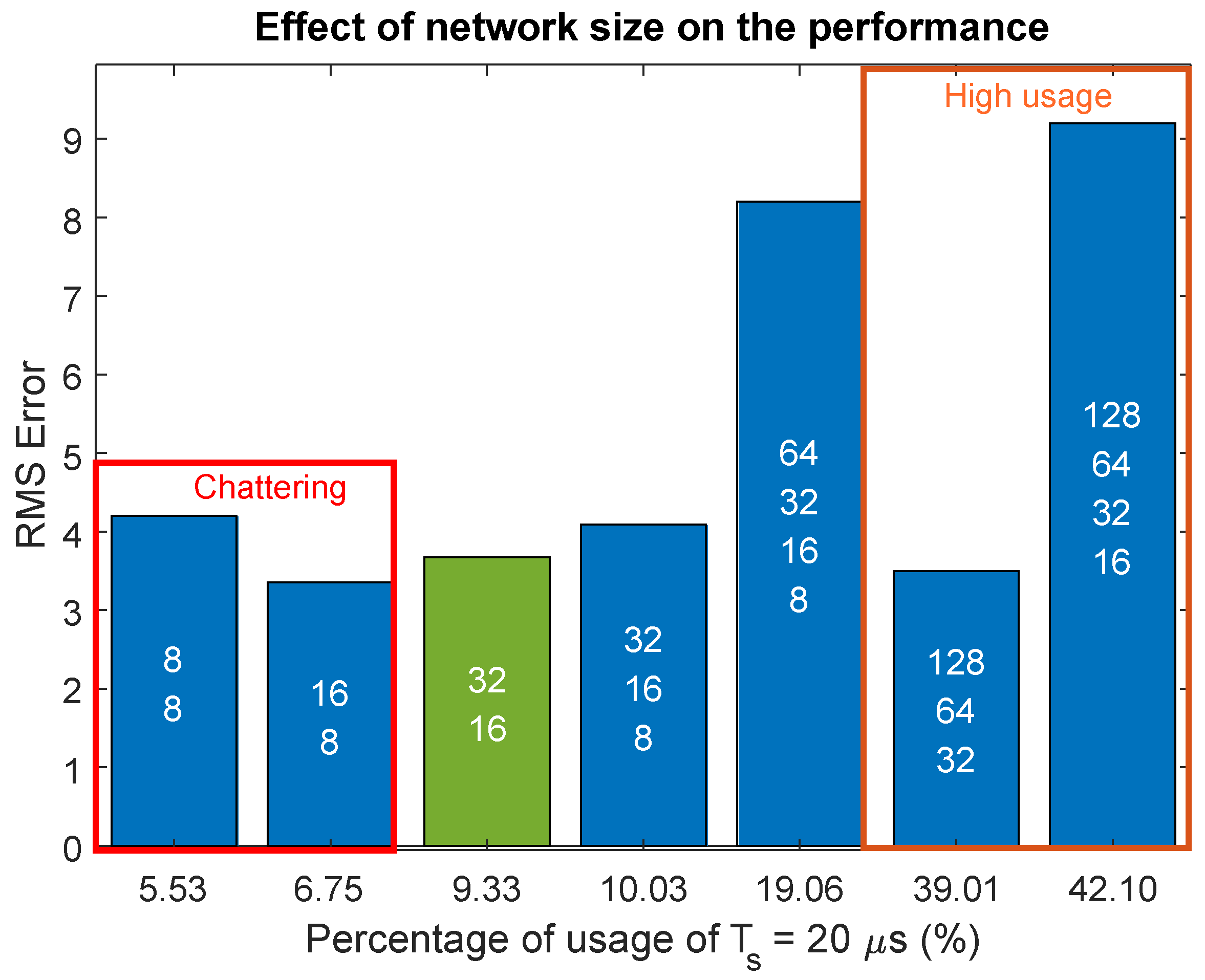
39]. Therefore, according to the trade-off analysis and the number of MACs, which will be presented in
Section 4.2.4, this network size configuration is chosen to achieve a balance between performance accuracy, computational complexity, and memory usage. Moreover, the input features vector relevant to
Table 2 consists of 19 components, including the output voltage, voltage tracking error, duty cycle, and the four previous values with a time step of
for each of them. Additionally, duty cycle variation, input voltage, integral gain, and reference voltage are part of the feature vector. The duty cycle is considered the action, making the ANN have one output and 19 inputs.
2.1.5. Training Procedure
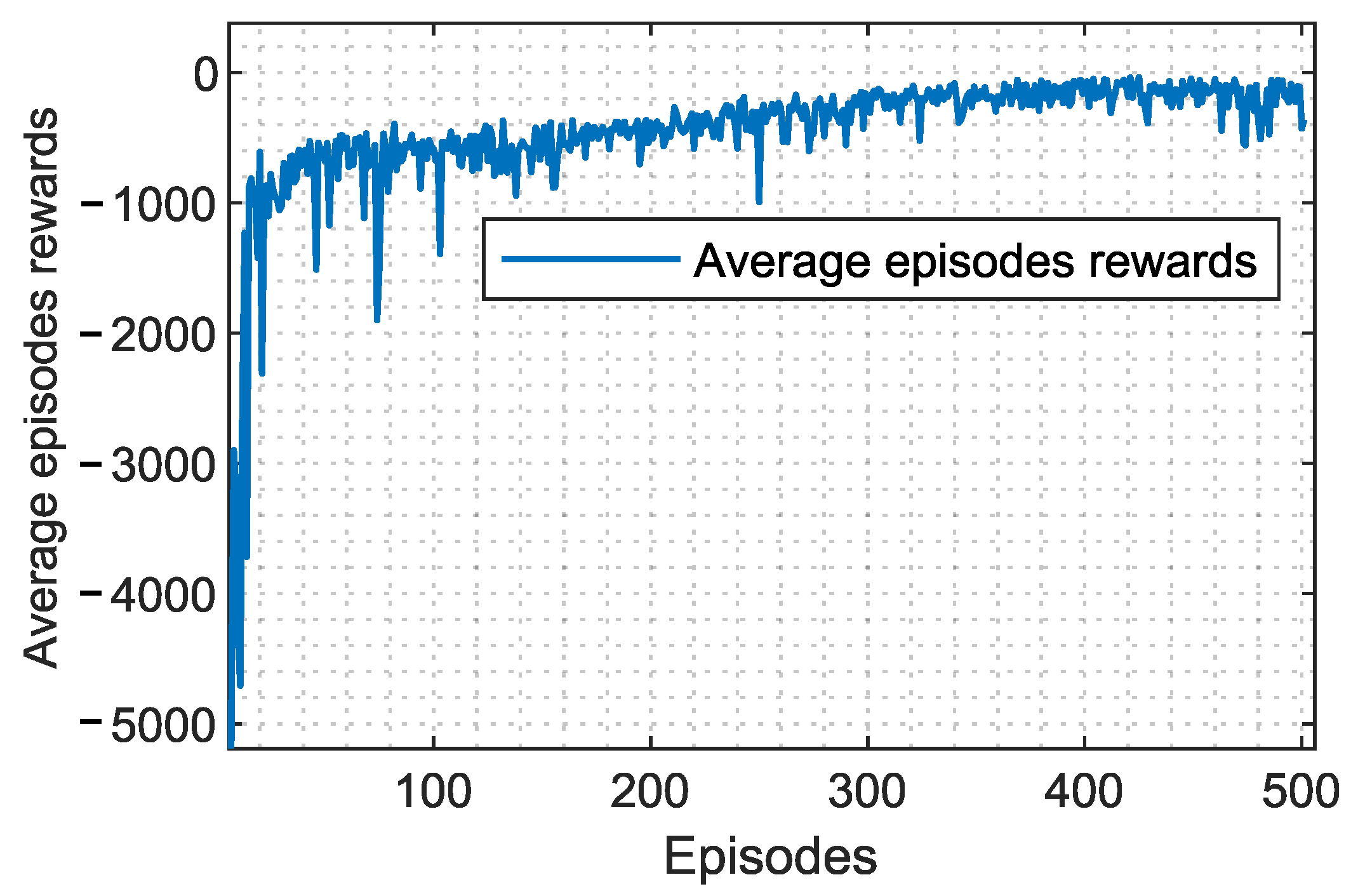
The training procedure for a PPO agent is designed to develop a policy that optimally interacts with an environment to achieve specific goals. The process begins with the agent exploring the environment, gathering state information that represents the current context and features variables, and then choosing an action based on its policy. Each action taken by the agent leads to a change in the environment, with the agent receiving a reward that indicates how favorable the outcome of that action was. The feedback from these rewards is important for learning and improving the policy. The key to PPO’s success lies in its ability to balance exploration and exploitation. Exploration involves trying new actions to gather information, while exploitation uses known strategies to maximize rewards. PPO achieves this balance through a unique clipped surrogate objective function, which helps to stabilize learning by limiting drastic changes to the policy. This approach, coupled with trust region optimization, ensures that the policy updates are smooth and controlled, reducing the risk of overfitting or oscillations during training. Throughout the training process, the agent collects a set of trajectories
, each consisting of a sequence of states, actions, rewards, and next states. These data are used to compute advantage estimates
, which help determine how much better or worse an action is compared to a baseline value function. The agent then uses these advantage estimates to update its policy through stochastic gradient descent, adjusting its decision-making strategy to improve performance. The iterative nature of PPO’s training process allows the agent to refine its policy over time, gradually increasing its ability to select actions that lead to better outcomes in the environment [
40,
41]. The pseudocode for the PPO-clipped algorithm, as shown in Algorithm 1, outlines the step-by-step procedure for implementing this approach [
34]. In this study, PPO-clipped is implemented, andcthe terms ‘PPO’ and ‘PPO-clipped’ are used interchangeably to refer to this algorithm.
Moreover, several hyperparameters need to be tuned appropriately to achieve the best possible performance and stability during training. These parameters play a crucial role in shaping various aspects of the learning process, such as the agent’s capacity to explore its environment and effectively exploit learned policies. Some of these hyperparameters are detailed in
Table 4, selected based on best practices and fine-tuned to address the specific challenges of the reinforcement learning problem and environment. Notably, the learning rate determines the magnitude of updates to the neural network’s weights during training. A higher learning rate may lead to faster convergence but risks overshooting the optimal policy, while a lower learning rate may result in slower convergence. To achieve a compromise between them, the value
is chosen. Similarly, the discount factor (gamma) influences the agent’s consideration of future rewards. A higher discount factor encourages long-term reward prioritization, while a lower value may prioritize immediate rewards. As a result, a value of 0.9 is selected. Additionally, the entropy coefficient plays a pivotal role in balancing exploration and exploitation by incentivizing the agent to explore novel actions. A higher entropy coefficient fosters exploration, whereas a lower coefficient emphasizes the exploitation of learned policies.
| Algorithm 1 PPO-clipped. |
- 1:
Input: Initial policy parameters , initial value function parameters - 2:
for
do - 3:
Collect the set of trajectories by running the policy in the environment. - 4:
Compute rewards-to-go, , representing the cumulative sum of future rewards from time step t onward. - 5:
Compute advantage estimates, (using any method of advantage estimation) based on the current value function which represents the expected return from a given state. - 6:
Update the policy by maximizing the PPO-clip objective:
typically, via stochastic gradient ascent with Adam. - 7:
Fit value function by regression on mean-squared error:
typically, via some gradient descent algorithm. - 8:
end for
|
3. A Practical Case: Implementation of the DRL Algorithm for a Buck Converter
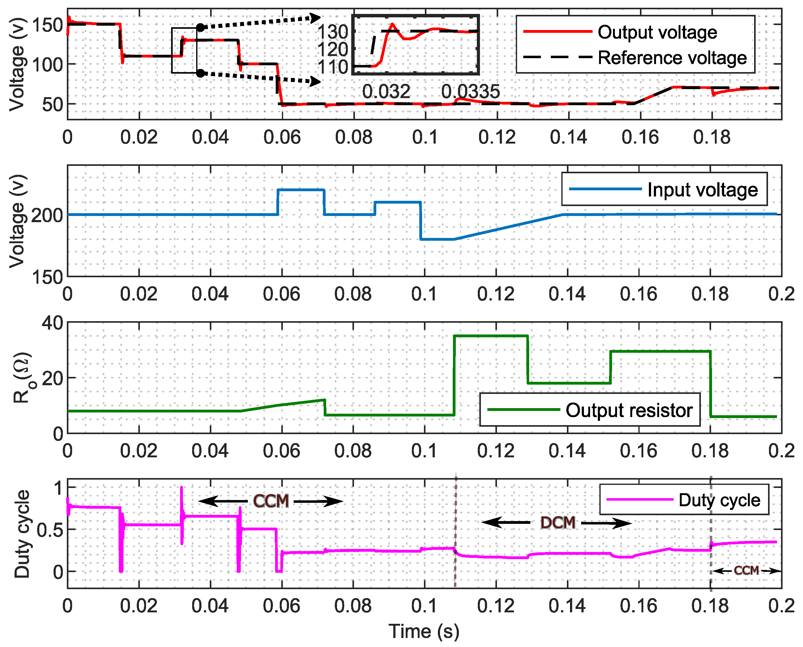
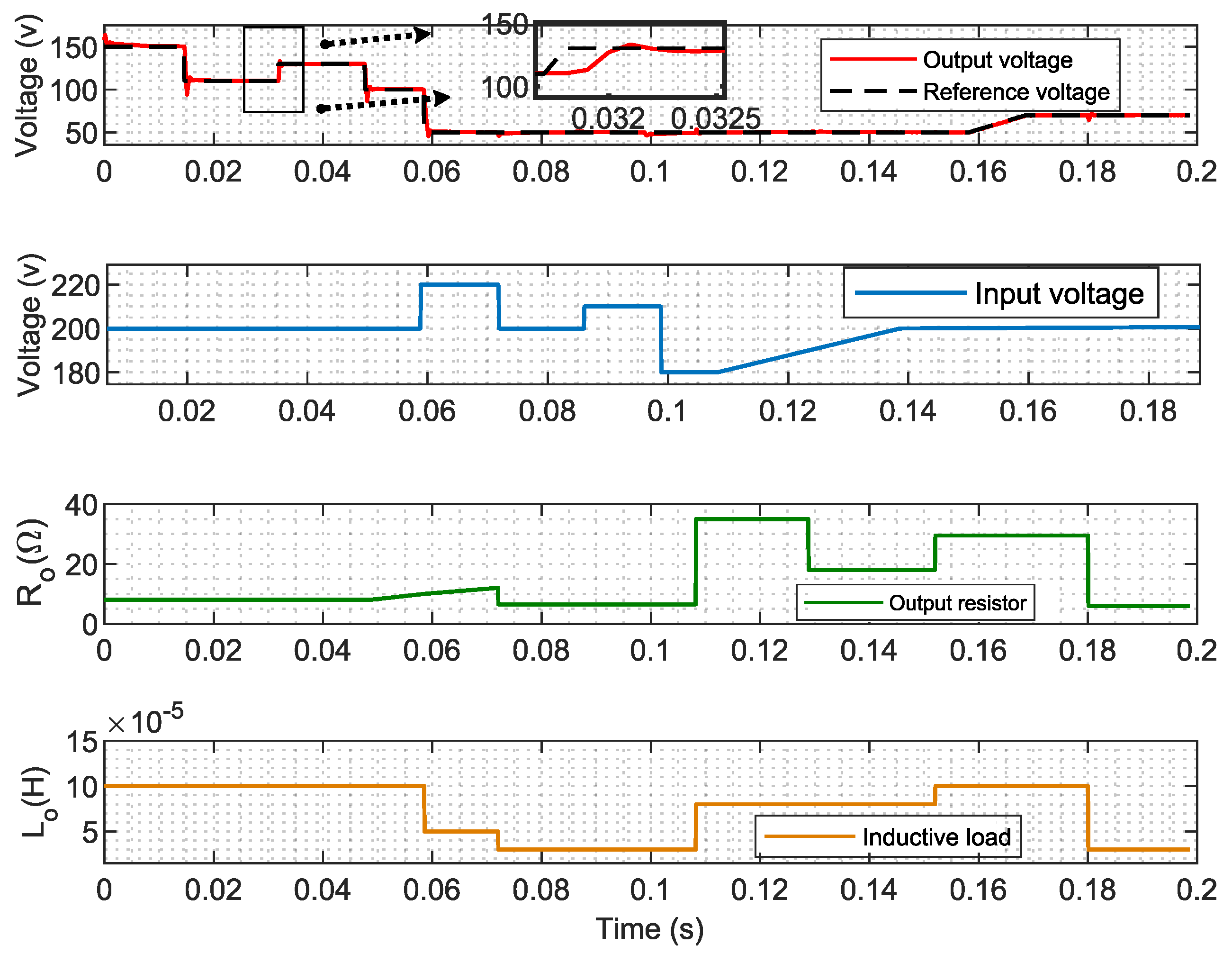
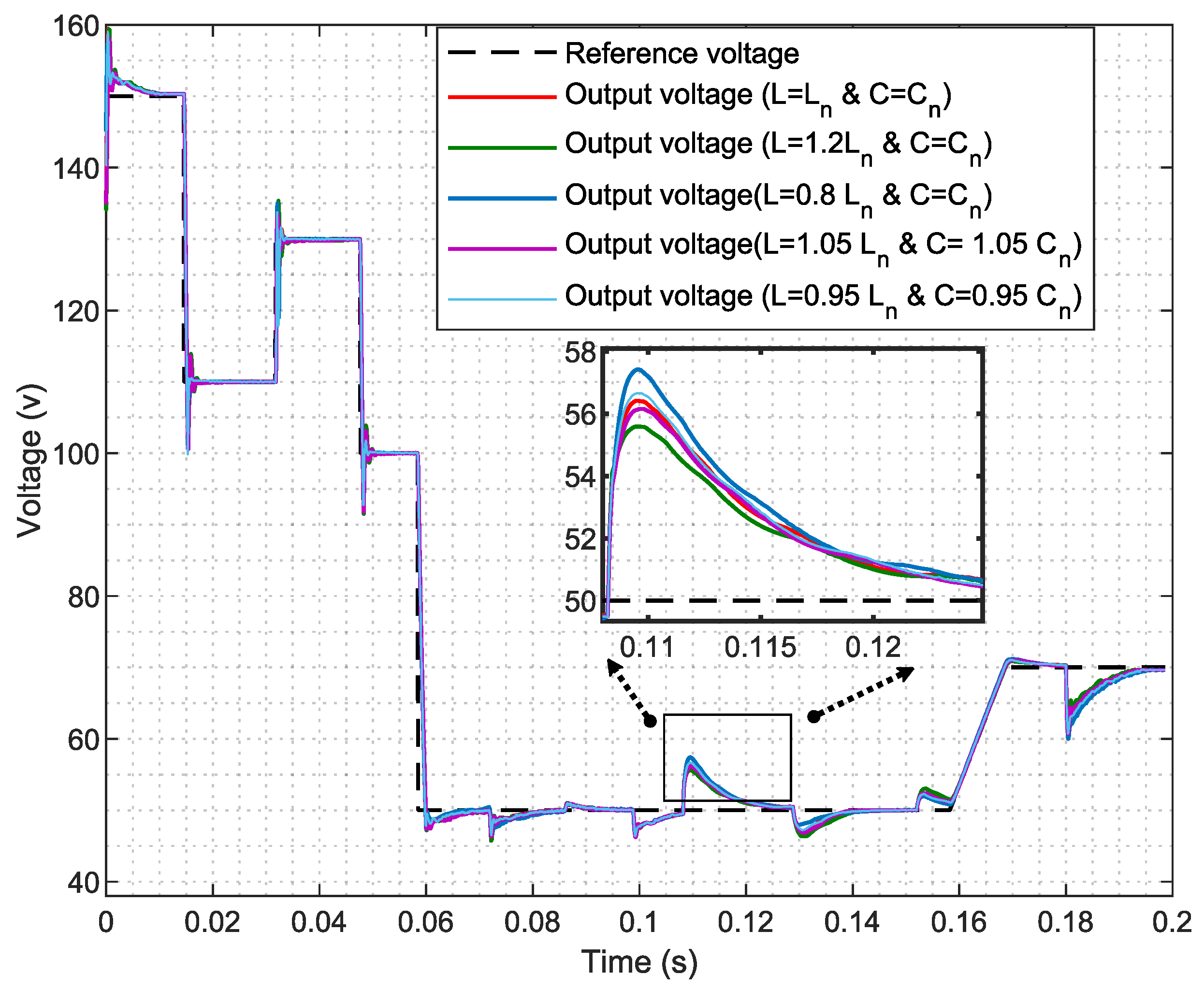
In this study, a real buck converter is used. Despite its simplicity, which facilitates understanding, it presents challenges due to its operation between DCM and CCM, leading to significant variations in the converter model. Additionally, the consideration of two types of loads, resistive and inductive, further complicates the analysis. This serves as the environment in which the agent interacts within the framework of DRL.
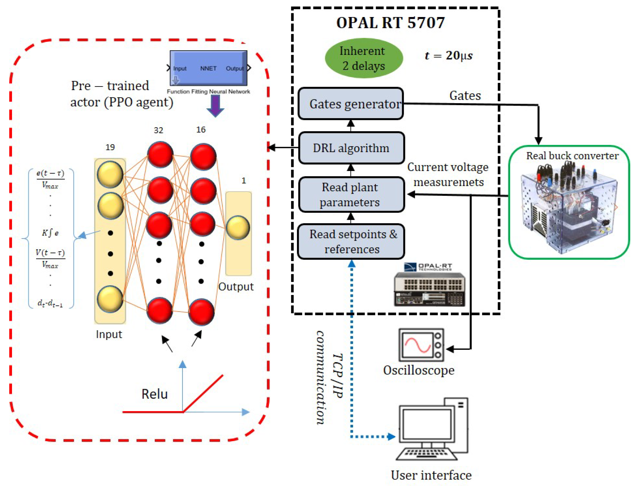
Figure 4 and
Figure 5 display the procedure of the PPO implementation in real-life scenarios. The architecture
is employed for the critic network, which is similar to the actor network. As illustrated in
Figure 4, Python 3.9 was chosen for its full-fledged support in designing DRL algorithms, leveraging its extensive libraries and frameworks. Meanwhile, the MATLAB 2023a Simulink environment is well-known for its powerful simulation capabilities, particularly in modeling dynamic systems such as power electronic converters. Additionally, the MATLAB Engine API facilitates seamless communication between Python and MATLAB for enhanced integration and efficiency. It is valuable to note that in the MATLAB Simulink environment, the choice of model and simulation program significantly impacts the accuracy of DC–DC power electronic converter simulations [
42]. In this study, the Simscape Electrical Specialized Power Systems toolbox within MATLAB/Simulink is selected due to its robustness and versatility in handling DC–DC power electronic simulations. Additionally, the use of the
PowerGui block with a time step of
(nanoseconds) ensures that high-frequency switching events are accurately resolved, providing precise insights into the converter’s transient and steady-state behavior. Moreover, it is notable that the PPO agent operates with a time step of
(microseconds). This time step was selected because the controller was designed to operate within the constraints of the real-time simulator OPAL-RT, which also uses a time step of
(microseconds). This synchronization ensures that the control actions are applied in real-time, maintaining the intended performance of the control system.
Introducing delays in a control system, especially when transitioning from simulation to real-time, can significantly impact performance. To address this, the PPO agent is trained in a detailed switching model that incorporates fixed delays of two time steps to accurately reflect real-time conditions.
Notably, the switching model includes the IGBT and diode module along with other elements of the buck converter simulation, as well as all considered parasitic elements, as provided in
Table 5 and
Table 6. Moreover,
Table 6 represents the parameters of the real buck converter used in the experimental tests, showing that the simulation parameters are similar to the real-time setup parameters.
It is important to note that the trained actor network, a key component of the PPO agent, is integrated and deployed as the controller within Simulink through the genism command in MATLAB.
