Switching Current Predictive Control of a Permanent Magnet Synchronous Motor Based on the Exponential Moving Average Algorithm

Abstract

To improve the dynamic and steady-state control performance of permanent magnet synchronous motors under the three-vector model predictive current control method, this study proposes a switching current predictive control method based on the exponential moving average algorithm, which evaluates the magnitude of the change of the q-axis current slope in real time to discriminate the motor’s operating conditions and selects the optimal control method for different operating conditions. Meanwhile, the traditional three-vector model predictive current control method is improved by introducing a comparison mechanism for the q-axis current slope to select the second effective voltage vector, avoiding the secondary optimization calculation of the value function and reducing the computational complexity of the traditional method. By comparing the proposed method with the traditional three-vector model predictive current control method, the experimental results prove that the proposed method improves the system’s dynamic response and steady-state performance.

1. Introduction

The operation of electric motors consumes about 46% of the total global electricity generation and emits about 640 million tonnes of carbon dioxide. Therefore, improving the energy efficiency of motors is essential for achieving energy savings, promoting environmental protection, and fostering sustainable development [1]. A Permanent Magnet Synchronous Motor (PMSM) has the advantages of high power density, small size, high efficiency, etc., and is widely used in various speed regulation fields [2]. Currently, there are two main control methods for PMSM: Field Oriented Control (FOC) [3] and Direct Torque Control (DTC) [4]. To achieve efficient digital control of a PMSM and improve the dynamic and steady-state control performance of the motor, both FOC control or DTC control have obvious drawbacks, and the traditional linear control methods are still insufficient under the multivariable, strongly coupled, and nonlinear characteristics of the PMSM system [5].

With the advancements in high-speed digital signal microprocessors like the Digital Signal Processor (DSP), there has been a significant boost in the computational power of control platforms in recent years. Model Predictive Control (MPC) has gained significant recognition in the motor control field due to its simple control structure, high flexibility, and fast dynamic response. It was ranked the top choice for advanced control algorithms in 2020 [6]. As a modern control theory, MPC is grounded in discrete control systems and involves the iterative optimization of future control variables based on the prediction model of the controlled system, along with feedback correction, to achieve optimal control efficacy [7]. In PMSM control applications, there are two types of MPC based on different control actions: Finite Control Set Model Predictive Control [8] (FCS-MPC) and Continuous Control Set Model Predictive Control [9] (CCS-MPC)—the main distinction between the two lies in the control system’s requirement for a modulation unit [10]. Using a discrete-time system model, FCS-MPC predicts the system’s future behavior for every potential switching voltage vector state. The optimal voltage vector is selected by evaluating all predictions using a value function [11]. Model Predictive Current Control (MPCC) for PMSM is an advanced method based on FCS-MPC. MPCC eliminates the need for parameter tuning in the current inner loop. Instead, it selects the optimal voltage vector using a value function in real-time. This approach bypasses pulse-width modulation and directly applies control signals to the motor system, streamlining the optimization and decision-making processes into a single step. However, traditional MPCC has limitations. It employs only one voltage vector per control cycle, with fixed direction and amplitude. This results in high current tracking error, significant current ripple, and poor steady-state control performance.

To solve this problem, scholars have proposed multi-vector MPCC [12], delay compensation [13], model-free control [14], etc. Among these methods, dual-vector model predictive current control (Dual-Vector MPCC, DV-MPCC) using two or three optimal voltage vectors to synthesize virtual voltage vectors or three-vector model predictive current control (Three-Vector MPCC, TV-MPCC) are the most widely used. Literature [15] designed a dual-vector computation method based on geometric theory for reference voltage vector sector judgment, which improves the steady-state current performance and effectively suppresses the zero-sequence current. However, the reference voltage vector sector’s judging procedure is intricate. Literature [16] selected the optimal voltage vector by calculating the intersection time between the q-axis current slopes at different voltage vectors and designing a cost function. However, each selection requires traversing all the primary voltage vectors, which is computationally intensive. Literature [17] updated the current slopes every half cycle after a model-free control method. It imposes two optimal voltage vectors in a single cycle, which can enhance the motor’s steady-state performance. However, the above DV-MPCC-based method has fewer effective voltage vector combinations, limiting the control accuracy and flexibility. Literature [18] employed a hierarchical multilevel optimization TV-MPCC method to reduce the current ripple. However, determining the first and second optimal voltage vectors is complex due to the intricate calculations required for the value function. Literature [19] selected the voltage vector under the stator flux closest to the CSF as the optimal voltage vector by determining the change in stator flux (Change in Stator-Flux, CSF) at each sampling. Literature [20] introduced the Romberg observer to estimate system perturbations, thereby reducing errors caused by motor parameter mismatches. Additionally, the candidate voltage vector combinations are reduced to two within a single sampling period, optimizing the selection of the optimal voltage vector. However, the multi-vector MPCC method leads to an increase in the switching frequency of the inverter, and to reduce the switching frequency, literature [21,22] proposed a dead-time voltage vector-based MPCC method, which reduces the switching loss of the inverter but increases the system complexity. Literature [23] used the optimal voltage vector in the previous control cycle as a reference for selecting the first voltage vector, which reduces the number of comparisons but only uses the speed error index to distinguish the dynamic and steady-state states of the motor from single and has limitations. Literature [24] designed a steady-state operation control method based on the four-segment mode MPC, which uses the average current slope to distinguish between the dynamic and steady-state states of the motor, which improves the steady-state performance and reduces the switching frequency at the same time, but the control logic is relatively complex.

Therefore, to improve the problems of extensive computation and poor system energy efficiency under the traditional TV-MPCC method, and at the same time, to further improve the control performance of TV-MPCC, this paper proposes to use the exponential moving average (EMA) algorithm for real-time updating of the reference threshold for the slope of the q-axis current and to use this threshold as a discriminative condition for differentiating the operating conditions of the motor, to adopt the most suitable control method according to the actual operating conditions of the motor.

The rest of the paper is organized as follows: Section 2 presents the mathematical model of PMSM. Section 3 describes the PMSM operating condition discrimination method based on the EMA algorithm. Section 4 describes the switching current prediction control method for the motor under different operating conditions and gives different control strategies under dynamic and steady-state operating conditions. Section 5 discusses the simulation and experimental results. Section 6 summarizes the conclusions of this paper.

2. Mathematical Model of PMSM

Based on the nonlinear and strongly coupled characteristics of the PMSM, and by ignoring some secondary factors, the stator voltage equation in the dq-axis synchronous rotating coordinate system of the PMSM in the ideal state is given by:

$$\left\{\begin{array}{l}{u}_d=R_s{i}_d+L_d{\displaystyle \frac{d{i}_d}{dt}}-{\omega }_e{L}_q{i}_q\\ u_q=R_s{i}_q+L_q{\displaystyle \frac{d{i}_q}{dt}}+{\omega }_e\left(L_d{i}_d+{\psi }_f\right)\end{array}\right.$$

(1)

where $u_d$ and $u_q$ are the stator dq-axis voltage components, $R_s$ is the stator resistances, $i_d$ and $i_q$ are the stator dq-axis current components, $L_d$ and $L_q$ are the dq-axis equivalent inductances, ${\omega }_e$ is the rotor angular velocity, and ${\psi }_f$ is the permanent magnet chains.

The PMSM mechanical equation of motion is:

$$J{\displaystyle \frac{d{\omega }_m}{dt}}=T_e-T_L-B{\omega }_m$$

(2)

where $J$ is the moment of inertia, ${\omega }_m$ is the mechanical angular velocity, $T_L$ is the load torque, and $B$ is the damping coefficient.

The experimental platform in this paper uses a surface-mounted permanent magnet synchronous motor (SPMSM). For this type of motor, $L_d=L_q=L_s$. Thus, the motor’s electromagnetic torque equation is:

$$T_e={\displaystyle \frac{3}{2}}{p}_n\left[{\psi }_f+\left(L_d-L_q\right)i_d\right]i_q={\displaystyle \frac{3}{2}}{p}_n{\psi }_f{i}_q$$

(3)

where $T_e$ is the electromagnetic torque, and $p_n$ is the number of pole pairs.

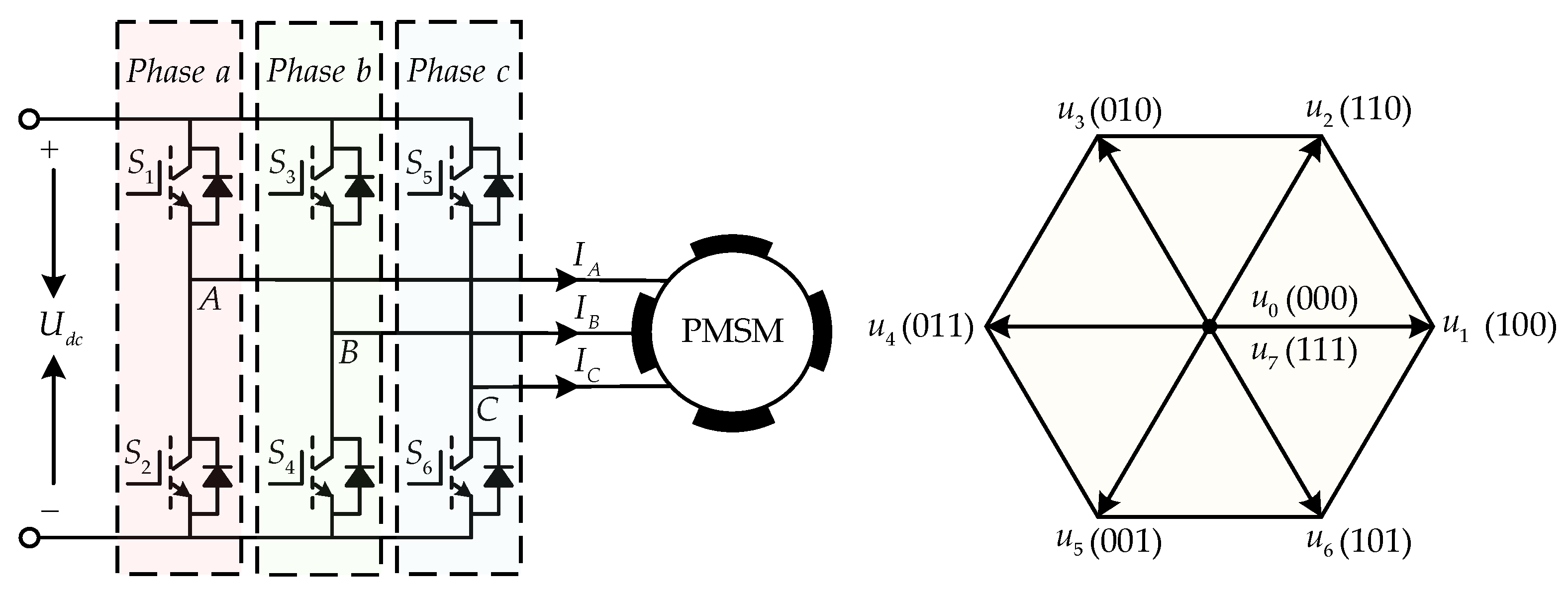
This paper utilizes a three-phase, two-level voltage source inverter (VSI) to control the basic voltage vector plane. The plane is divided into six sectors, each containing two zero vectors and six effective voltage vectors. The circuit topology and distribution of the basic voltage vectors are illustrated in Figure 1.

3. PMSM Operation Status Judgment

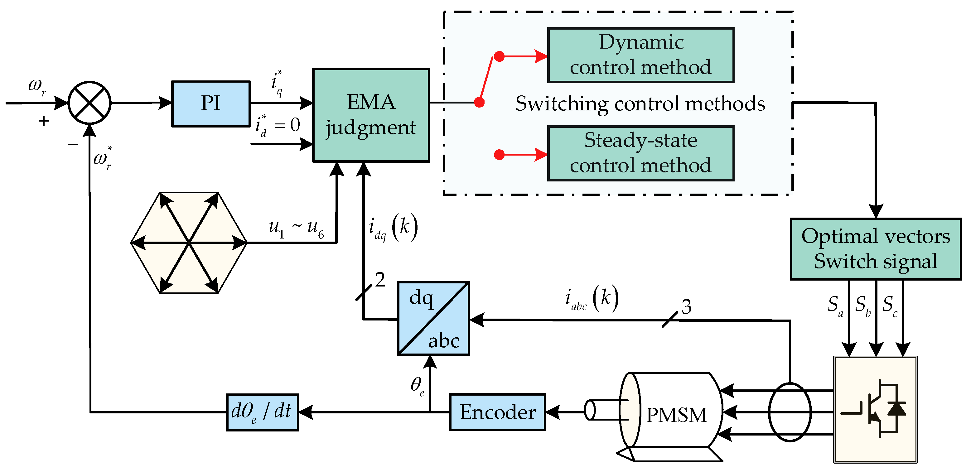
This section proposes the discriminative conditions of PMSM operation states, and different control methods are adopted for different operation states. The improved three-vector steady-state operation current prediction control method is employed when the motor is in the steady-state mode, and the improved Dual-vector dynamic operation current prediction control method is applied when the motor is in the dynamic mode. Figure 2 shows the control block diagram.

3.1. Slope of q-Axis Current to Determine the Operating State of the Motor

To achieve the best performance, PMSM requires different control strategies under different operating conditions. Specifically, when the motor is in dynamic operation, the system needs a fast dynamic response time to adapt to different operating conditions. The system must maintain good current steady-state performance when the motor is in steady-state operation.

The discrete dq-axis current prediction equation for the next sampling moment is obtained by approximating (1) with the first-order Eulerian discretization method:

$$\left\{\begin{array}{l}{i}_d\left(k+1\right)=i_d\left(k\right)+{\displaystyle \frac{T_s}{L_s}}\left[u_d\left(k\right)-R_s{i}_d\left(k\right)+E_d\left(k\right)\right]\\ i_q\left(k+1\right)=i_q\left(k\right)+{\displaystyle \frac{T_s}{L_s}}\left[u_q\left(k\right)-R_s{i}_q\left(k\right)+E_q\left(k\right)\right]\end{array}\right.$$

(4)

where:

$$\left\{\begin{array}{l}{E}_d\left(k\right)={\omega }_e\left(k\right)L_s{i}_q\left(k\right)\hfill \\ E_q\left(k\right)=-{\omega }_e\left(k\right)\left[L_s{i}_d\left(k\right)+{\psi }_f\right]\hfill \end{array}\right.$$

(5)

where $i_d\left(k+1\right)$ and $i_q\left(k+1\right)$ are the predicted value of dq-axis current at the moment k + 1, $i_d\left(k\right)$ and $i_q\left(k\right)$ are the value of dq-axis current at the moment k, $T_s$ is the sampling period, $u_d\left(k\right)$ and $u_q\left(k\right)$ are the dq-axis voltage at the moment k, $E_d\left(k\right)$ and $E_q\left(k\right)$ are the dq-axis inverse potential at the moment k, respectively.

The motor will operate dynamically when the PMSM speed or load torque changes abruptly. From (2), when the motor load or speed changes suddenly, the electromagnetic torque will also change accordingly, and from (3), the electromagnetic torque is positively correlated with the q-axis current, and when the q-axis current changes suddenly, there is a significant change in its slope. Therefore, the change of electromagnetic torque can be judged by the change of the slope of the q-axis current, which leads to the conclusion that whether the motor is switched to the dynamic state can be judged by the change of the slope of the q-axis current.

The slope of the dq-axis current under the action of $u_1~u_6$ can be obtained from (1):

$$\left\{\begin{array}{l}{S}_d={\displaystyle \frac{1}{L_s}}\left[-R_s{i}_d\left(k\right)+{\omega }_e{L}_s{i}_q\left(k\right)+u_d\left(k\right)\right]\\ S_q={\displaystyle \frac{1}{L_s}}\left[-R_s{i}_d\left(k\right)-{\omega }_e{L}_s{i}_d\left(k\right)-{\omega }_e{\psi }_f+u_q\left(k\right)\right]\end{array}\right.$$

(6)

where $S_d$ and $S_q$ are the dq-axis current slopes of $u_1~u_6$ at moment k, respectively.

Thus, the slope of the dq-axis current under the action of $u_0$ and $u_7$ can be obtained:

$$\left\{\begin{array}{l}{S}_{d0}=S_{d7}={\displaystyle \frac{1}{L_s}}\left[-R_s{i}_d\left(k\right)+{\omega }_e{L}_s{i}_q\left(k\right)\right]\\ S_{q0}=S_{q7}={\displaystyle \frac{1}{L_s}}\left[-R_s{i}_d\left(k\right)-{\omega }_e{L}_s{i}_d\left(k\right)-{\omega }_e{\psi }_f\right]\end{array}\right.$$

(7)

where $S_{d0}$,$S_{d7}$,$S_{q0}$,$S_{q7}$ are the dq-axis current slopes of $u_0$ and $u_7$ at moment k, respectively.

The value function is constructed, and the candidate voltage vector that minimizes the value function value is selected as the first effective voltage vector $u_{opt1}$ among the six effective voltage vectors and the constructed value function $g_i$ is:

$$g_i={\left[i_d^{*}-i_d\left(k+1\right)\right]}^2+{\left[i_q^{*}-i_q\left(k+1\right)\right]}^2$$

(8)

where $i_d^{*}$ is the given value of the stator current d-axis component, and $i_q^{*}$ is the given value of the stator current q-axis component.

Employing the value function set in (8), the six effective voltage vectors are traversed, and the dq-axis reference voltage under action is obtained by the Park transform:

$$\left\{\begin{array}{l}{u}_{d-ref}^{*}=u_{\alpha -ref}^{*}\cos \left({\theta }_e\right)+u_{\beta -ref}^{*}\sin \left({\theta }_e\right)\hfill \\ u_{q-ref}^{*}=-u_{\alpha -ref}^{*}\sin \left({\theta }_e\right)+u_{\beta -ref}^{*}\cos \left({\theta }_e\right)\hfill \end{array}\right.$$

(9)

where ${\theta }_e$ is the angle between the d-axis and the shaft, $u_{\alpha -ref}^{*}$ and $u_{\beta -ref}^{*}$ are the shaft reference voltage under $u_{opt1}$ action, and $u_{d-ref}^{*}$ and $u_{q-ref}^{*}$ are the dq-axis reference voltage under $u_{opt1}$ action.

The dq-axis current slope under the action of $u_{opt1}$ is used as the q-axis current slope for discriminating the motor operating state:

$$\left\{\begin{array}{l}{S}_{d-opt1}=S_{d0}+{\displaystyle \frac{u_{d-ref}^{*}}{L_s}}\\ S_{q-opt1}=S_{q0}+{\displaystyle \frac{u_{q-ref}^{*}}{L_s}}\end{array}\right.$$

(10)

3.2. Motor Operating Condition Discrimination Based on the EMA Algorithm

EMA is a technical algorithm in the time series analysis of data methods, which can give more weight to recent data points in calculating the average, effectively capturing the latest trend of data changes and reducing the lagging effect and short-term fluctuations in the impact of data. The equation for the EMA algorithm is:

$$v_k=\alpha v_{k-1}+\left(1-\alpha \right){\theta }_k$$

(11)

where $v_k$ and $v_{k-1}$ are the values of the EMA at moment k and k − 1, ${\theta }_k$ is the actual observation at the moment k, and $\alpha \in [0,1]$ is the smoothing factor.

The EMA algorithm is simple and small in computation, which is suitable for real-time processing requirements of embedded systems and does not overburden the system resources. Therefore, the EMA method based on the q-axis current slope is introduced to accurately judge the motor running state. Through the real-time updated q-axis current slope, it quickly responds to the motor state changes and improves the accuracy of judging the motor running state.

Based on the above analysis, $u_{opt1}$ is first obtained from the value function shown in (8), and under the action of $u_{opt1}$, the updated formula of EMA is:

$$S_{EMA-q}\left(k\right)=\alpha S_{q-opt1}\left(k\right)+\left(1-\alpha \right)S_{EMA-q}\left(k-1\right)$$

(12)

where $S_{EMA-q}\left(k\right)$ and $S_{EMA-q}\left(k-1\right)$ are the value of the q-axis current slope EMA at the moment k and k − 1, and $S_{q-opt1}\left(k\right)$ is the actual observation of the q-axis current slope.

At the instant of motor startup, the rotational speed is increased from zero in either loaded or unloaded state, and the process before the motor rises to the target rotational speed is a dynamic control operation. Therefore, if the stationary state of the motor is set as the initial state of the designed current model predictive toggle switch control method, the default initial state of the control method should be steady-state operation control.

To accurately track the instantaneous changes in the motor state and to achieve a fast response to its state switching, the difference between $S_{q-opt1}\left(k\right)$ at the moment k and $S_{EMA-q}\left(k\right)$ under the EMA method is defined as a real-time indicator for tracking the change in the slope of the q-axis current:

$$e_q=S_{q-opt1}-S_{EMA-q}$$

(13)

From (13), if $e_q$ changes during motor startup and operation, the slope of the q-axis current changes. In order to avoid the system switching the control method frequently due to too small a change of current slope, it is necessary to set a dynamic threshold to adapt to the change of the motor operation state in real-time; at the same time, based on the dynamic threshold having the characteristic of non-negativity, it can be expressed as follows:

$$\lambda =\beta \left|S_{EMA-q}\right|$$

(14)

where $\lambda$ is the dynamic threshold for switching the motor operating state, and $\beta$ is the scaling factor.

In the study of this paper, the discrimination of the motor running state is based on the real-time change amplitude of the q-axis current slope, which only focuses on the magnitude size of the change rather than the direction of its change. Therefore, in order to quantify the magnitude of the change, a motor operation state index $\delta$ is introduced to discriminate the operation state of the motor, which can be obtained from (13) and (14):

$$\delta =\left|e_q\right|-\lambda$$

(15)

where $\delta$ is the motor operating status indicator.

If $\delta >0$, it means that the q-axis current change rate of the motor exceeds the set threshold range, and at this time, the motor adopts the dynamic operation control method; if $\delta \le 0$, it means that the current change rate of the motor is small, and at this time the motor adopts the steady-state operation control method.

Figure 3 shows the control block diagram of the discriminating method of the motor operation state. Firstly, the optimal voltage vector $u_{opt1}$ is calculated by the reference value and predicted value of the dq-axis current, then $S_{q-opt1}\left(k\right)$ is obtained, and finally, the motor working condition is discriminated according to the set value of the motor operation index.

4. Switching Current Predictive Control

According to the EMA method based on the slope of the q-axis current proposed in the previous section, after discriminating the operating conditions of the motor, different current prediction control methods are switched for different operating states to improve the control performance of the system.

4.1. Dynamic Operational Control Method

When the PMSM is in dynamic operation, its speed or load will change abruptly. In order to make the control system have a fast-tracking response, only one optimal effective voltage vector and one optimal zero vector are used in each sampling cycle. To simplify the voltage vector selection process, reduce switching losses, and reduce current fluctuations due to frequent switching of voltage vectors, the optimal effective voltage vector selected by the value function is acted on twice, i.e., the first voltage vector is the same as the second voltage vector under the dynamic operation control method:

$$u_{opt1}=u_{d-opt1}=u_{d-opt2}$$

(16)

where $u_{d-opt1}$ and $u_{d-opt2}$ are the first and second effective voltage vectors under the dynamic operation control method, respectively.

A set value function traverses the six effective voltage vectors, and the dq-axis reference voltage under the action of $u_{d-opt1}$ is obtained by the Park transform:

$$\left\{\begin{array}{l}{u}_{d1-ref}^{*}=u_{\alpha 1-ref}^{*}\cos \left({\theta }_e\right)+u_{\beta 1-ref}^{*}\sin \left({\theta }_e\right)\hfill \\ u_{q1-ref}^{*}=-u_{\alpha 1-ref}^{*}\sin \left({\theta }_e\right)+u_{\beta 1-ref}^{*}\cos \left({\theta }_e\right)\hfill \end{array}\right.$$

(17)

where ${\theta }_e$ is the angle between the d-axis and the shaft, $u_{\alpha 1-ref}^{*}$ and $u_{\beta 1-ref}^{*}$ are the shaft reference voltage under action $u_{d-opt1}$, and $u_{d1-ref}^{*}$ and $u_{q1-ref}^{*}$ are the dq-axis reference voltage under action $u_{d-opt1}$.

The slope of the dq-axis current when $u_{d-opt1}$ acts:

$$\left\{\begin{array}{l}{S}_{di}=S_{d0}+{\displaystyle \frac{u_{d1-ref}^{*}}{L_s}}\\ S_{qi}=S_{q0}+{\displaystyle \frac{u_{q1-ref}^{*}}{L_s}}\end{array}\right.$$

(18)

The optimal zero vector $u_{d-opt3}$ under the dynamic operation control is selected based on minimizing the number of switch transitions while using the $u_{d-opt1}$.

Table 1. Optimal voltage vector selection under the dynamic operational control method.

${\mathit{u}}_{\mathit{d}-\mathit{o}\mathit{p}\mathit{t}\mathbf{1}}={\mathit{u}}_{\mathit{d}-\mathit{o}\mathit{p}\mathit{t}\mathbf{2}}$	${\mathit{u}}_{\mathit{d}-\mathit{o}\mathit{p}\mathit{t}\mathbf{3}}$
$u_1$(100), $u_3$(010), $u_5$(001)	$u_0$(000)
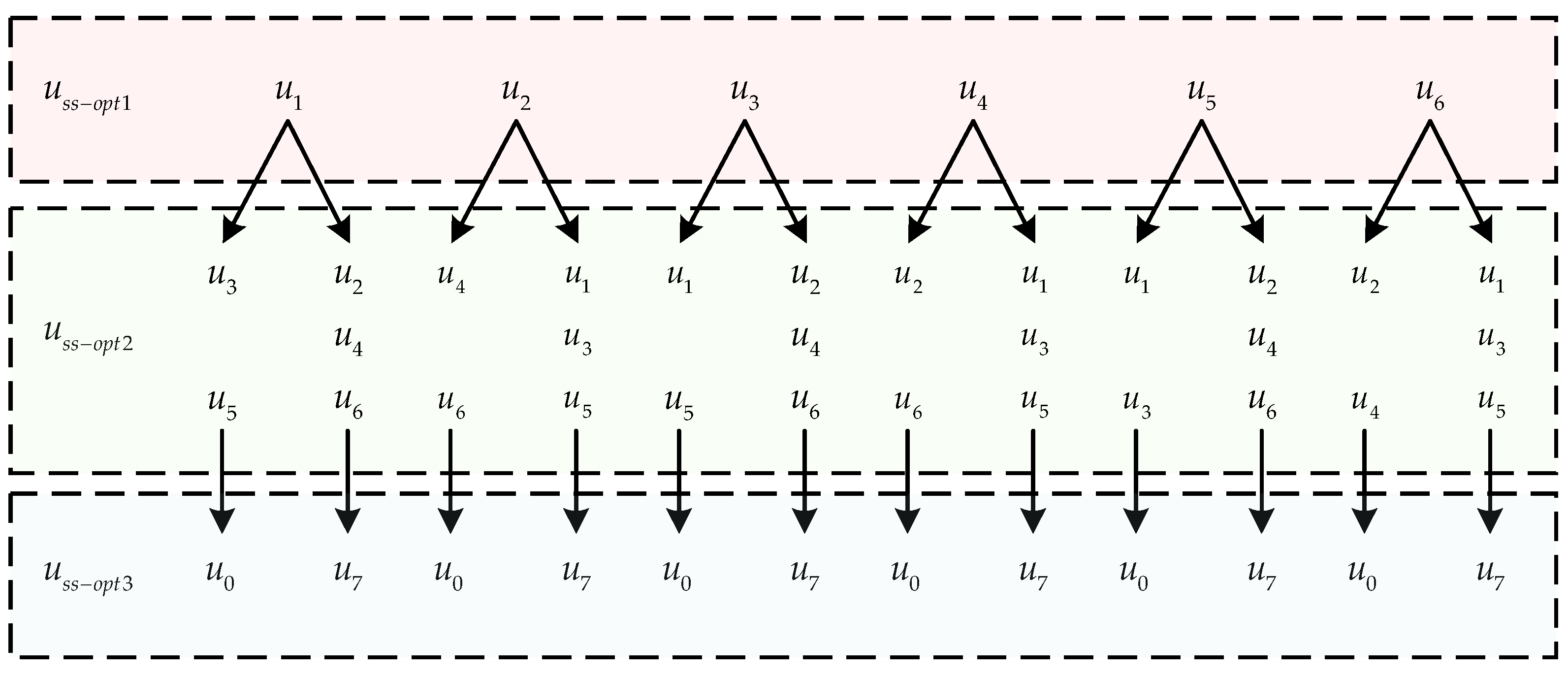
$u_2$(110), $u_4$(011), $u_6$(101)	$u_7$(111)

shows the optimal voltage vector selection table for the motor under dynamic operating conditions.

4.2. Steady-State Operation Control Method

When the PMSM is in steady-state operation, its speed or load remains stable. At this point, the control technique should prioritize steady-state performance over rapid response. Additionally, decreasing system computation is vital, which can be accomplished by employing a feedback selection mechanism depending on the q-axis current slope. This control approach employs two effective voltage vectors and one optimal zero vector in each sampling cycle. Figure 4 shows the control block diagram for this strategy.

4.2.1. The q-Axis Current Reference Slope and Optimum Voltage Vector’s Action Time Calculations

To select the second effective voltage vector $u_{ss-opt2}$ under the steady-state operation control method in real-time and track the current trajectory more accurately, $u_{ss-opt1}$ and zero voltage vectors are first excluded, and the remaining five effective voltage vectors are traversed as candidate voltage vectors. To choose the second effective voltage vector $u_{ss-opt2}$, compute the q-axis current slope magnitude under the influence of five candidate voltage vectors and create a reference magnitude for the q-axis current slope.

The dq-axis reference voltage and dq-axis current slopes after traversing the candidate voltage vectors are obtained by using the Park transform:

$$\left\{\begin{array}{l}{u}_{d2-ref}^{*}=u_{\alpha 2-ref}^{*}\cos \left({\theta }_e\right)+u_{\beta 2-ref}^{*}\sin \left({\theta }_e\right)\hfill \\ u_{q2-ref}^{*}=-u_{\alpha 2-ref}^{*}\sin \left({\theta }_e\right)+u_{\beta 2-ref}^{*}\cos \left({\theta }_e\right)\hfill \end{array}\right.$$

(19)

$$\left\{\begin{array}{l}{S}_{dj}=S_{d0}+{\displaystyle \frac{u_{d2-ref}^{*}}{L_s}}\\ S_{qj}=S_{q0}+{\displaystyle \frac{u_{q2-ref}^{*}}{L_s}}\end{array}\right.$$

(20)

where $u_{\alpha 2-ref}^{*}$ and $u_{\beta 2-ref}^{*}$ are the $\alpha \beta$-axis reference voltages of the candidate vectors, $u_{d2-ref}^{*}$ and $u_{q2-ref}^{*}$ are the dq-axis reference voltage of the candidate vectors, and $S_{dj}$ and $S_{qj}$ are the dq-axis current slopes of the candidate vectors, respectively.

To track the reference given value of the q-axis current slope in the next control cycle without error, the action time of each optimal voltage vector is calculated according to the principle of dead-beat control so that the predicted value of the dq-axis current is the same as that of the reference given value, which yields the following equations for $i_d\left(k+1\right)$ and $i_d\left(k\right)$ under the three-vector model predictive current control:

$$\left\{\begin{array}{l}{i}_d\left(k+1\right)=i_d^{*}=i_d\left(k\right){+\mathrm{S}}_{di}{t}_i+{\mathrm{S}}_{dj}{t}_j+{\mathrm{S}}_{d0}{t}_z\\ i_q\left(k+1\right)=i_q^{*}=i_q\left(k\right){+\mathrm{S}}_{qi}{t}_i+{\mathrm{S}}_{qj}{t}_j+{\mathrm{S}}_{q0}{t}_z\end{array}\right.$$

(21)

$$T_s=t_i+t_j+t_z$$

(22)

where $t_i$, $t_j$, and $t_z$ are the action times of the optimal zero voltage vector for $u_{ss-opt1}$ and $u_{ss-opt2}$, respectively.

The three optimal voltage vectors are modulated in order to ensure that the motor’s current error averages out to zero in each action cycle:

$$\left\{\begin{array}{l}\left[i_d^{*}-i_d\left(k\right)\right]T_s=0\\ \left[i_q^{*}-i_q\left(k\right)\right]T_s=0\end{array}\right.$$

(23)

According to (21)–(23), the optimal voltage vector action time of the motor in each control cycle is obtained as follows:

$$\left\{\begin{array}{l}{t}_i={\displaystyle \frac{\left[i_q^{*}-i_q\left(k\right)\right]\left(S_{d0}-S_{dj}\right)+\left[i_d^{*}-i_d\left(k\right)\right]\left(S_{qj}-S_{q0}\right)+T_s\left(S_{dj}{S}_{q0}-S_{d0}{S}_{qj}\right)}{S_{dj}{S}_{q0}-S_{di}{S}_{q0}+S_{d0}{S}_{qi}-S_{d0}{S}_{qj}+S_{di}{S}_{qj}-S_{dj}{S}_{qi}}}\\ t_j={\displaystyle \frac{\left[i_d^{*}-i_d\left(k\right)\right]\left(S_{q0}-S_{qi}\right)+\left[i_q^{*}-i_q\left(k\right)\right]\left(S_{di}-S_{d0}\right)-T_s\left(S_{dj}{S}_{q0}-S_{d0}{S}_{qi}\right)}{S_{dj}{S}_{q0}-S_{di}{S}_{q0}+S_{d0}{S}_{qi}-S_{d0}{S}_{qj}+S_{di}{S}_{qj}-S_{dj}{S}_{qi}}}\\ t_z=T_s-t_i-t_j\end{array}\right.$$

(24)

In the steady-state condition, the state of the motor changes less, and the current tends to a stable value. In a single control cycle, the optimal voltage vector action time for the desired modulation is always in the range $0~T_s$. Otherwise, the action time needs to be corrected. If the time is 0, it means that the voltage vector is discarded in that action cycle, as shown in

Table 2. Optimal voltage vector action time.

Original Action Time	Corrected Action Time
$t_i\in \left[0,T_s\right]$$, t_j\in \left[0,T_s\right]$$, t_z\notin \left[0,T_s\right]$	$t_i=t_i$$, t_j=t_j$$, t_z=0$
$t_i\in \left[0,T_s\right]$$, t_j\notin \left[0,T_s\right]$$, t_z\in \left[0,T_s\right]$	$t_i=t_i$$, t_j=0$$, t_z=t_z$
$t_i\notin \left[0,T_s\right]$$, t_j\in \left[0,T_s\right]$$, t_z\in \left[0,T_s\right]$	$t_i=0$$, t_j=t_j$$, t_z=t_z$
$t_i\in \left[0,T_s\right]$$, t_j\notin \left[0,T_s\right]$$, t_z\notin \left[0,T_s\right]$	$t_i=T_s$$, t_j=0$$, t_z=0$
$t_i\notin \left[0,T_s\right]$$, t_j\in \left[0,T_s\right]$$, t_z\notin \left[0,T_s\right]$	$t_i=0$$, t_j=T_s$$, t_z=0$
$t_i\in \left[0,T_s\right]$$, t_j\in \left[0,T_s\right]$$, t_z\in \left[0,T_s\right]$	$t_i=t_i$$, t_j=t_j$$, t_z=t_z$

:

From (5), the motor changes the dq-axis current slope after one cycle of each effective voltage vector action. Using the principle of dead-beat control, the q-axis reference predicted current magnitude is made to be the same as the current reference given magnitude at the current moment, which is given by the following equation:

$$\left|i_{q-ref}\left(k+1\right)\right|=\left|i_{q-ref}^{*}\left(k+1\right)\right|=\left|i_q\left(k\right)+{\displaystyle \frac{T_s}{L_s}}\left[u_{q1-ref}^{*}{\displaystyle \frac{t_i}{T_s}}+u_{q2-ref}^{*}{\displaystyle \frac{t_j}{T_s}}-R_s{i}_q\left(k\right)+E_q\left(k\right)\right]\right|$$

(25)

where $i_{q-ref}\left(k+1\right)$ is the reference predicted amplitude of the q-axis current at moment k + 1, $i_{q-ref}^{*}\left(k+1\right)$ is the reference given amplitude of the q-axis current at moment k + 1.

The reference amplitude of the q-axis current slope is obtained from (25):

$$S_q^{ref}={\displaystyle \frac{\left|i_{q-ref}^{*}\left(k+1\right)\right|-\left|i_q^{*}\right|}{T_s}}$$

(26)

4.2.2. Selection of Optimum Voltage Vector

The optimal effective voltage vector selected under the dynamic operation control method is used as the first optimal effective voltage vector $u_{ss-opt1}$ under the steady-state operation control method to maintain the continuity of system control.

In determining the second optimal effective voltage vector $u_{ss-opt2}$, the zero-voltage vector is first excluded, at which point five candidate effective voltage vectors remain. The q-axis current slope amplitude $S_{qj}$ under the five candidate voltage vectors is compared with the q-axis current reference slope amplitude $S_q^{ref}$. The slope amplitude closest to $S_q^{ref}$ is selected, and the voltage vector acting on this slope amplitude is determined, which is the desired second optimal effective voltage vector $u_{ss-opt2}$.

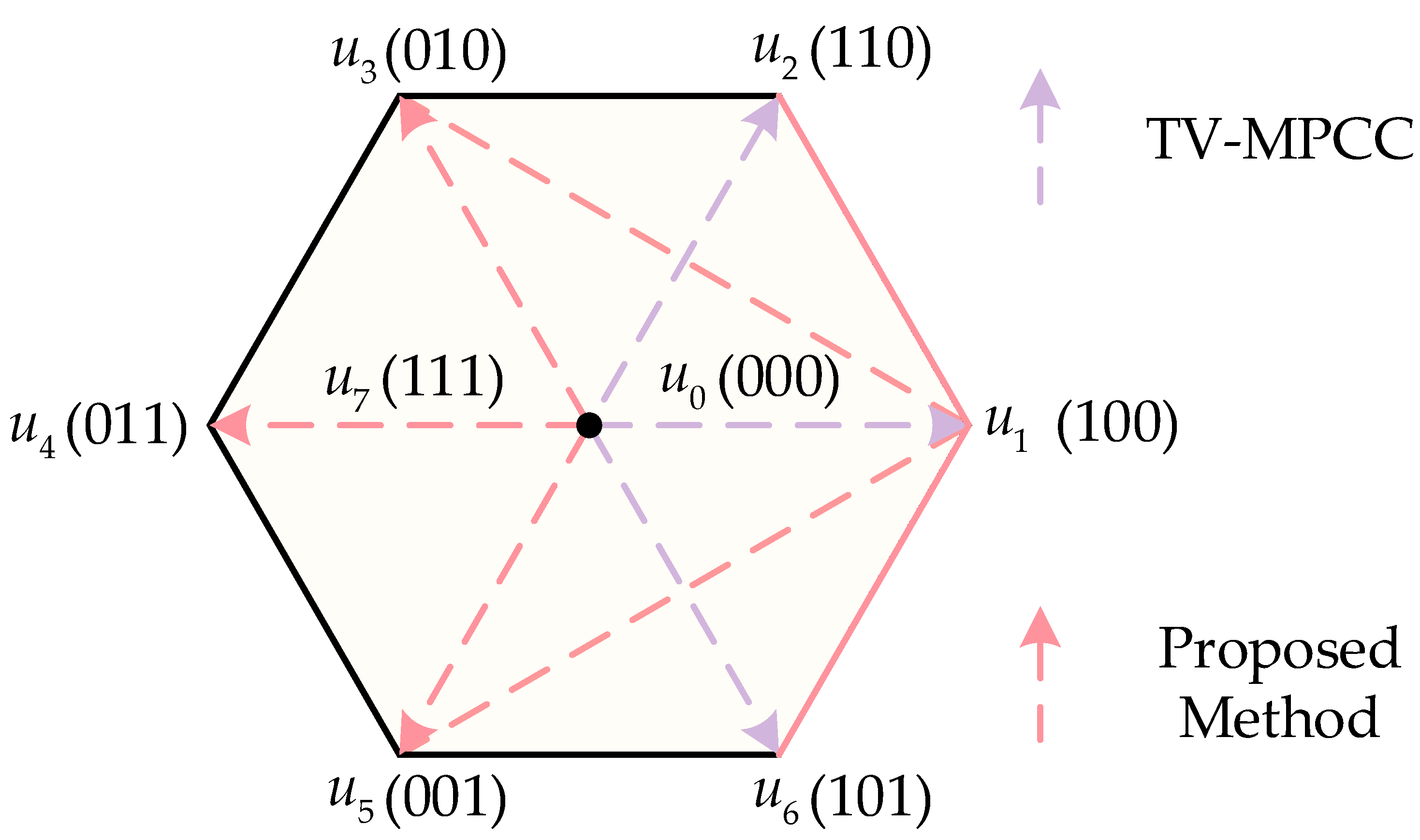
Figure 5 shows the coverage of the virtual voltage vectors of the conventional TV-MPCC method and the proposed method. As seen in Figure 5, the alternative voltage vector range of the traditional method contains only two neighboring voltage vectors and the zero vector, which limits the control system’s coverage and flexibility. In contrast, the proposed method can select the optimal vector among all the voltage vectors, which expands the coverage of the synthesized virtual voltage vectors based on the traditional method and improves the system’s performance.

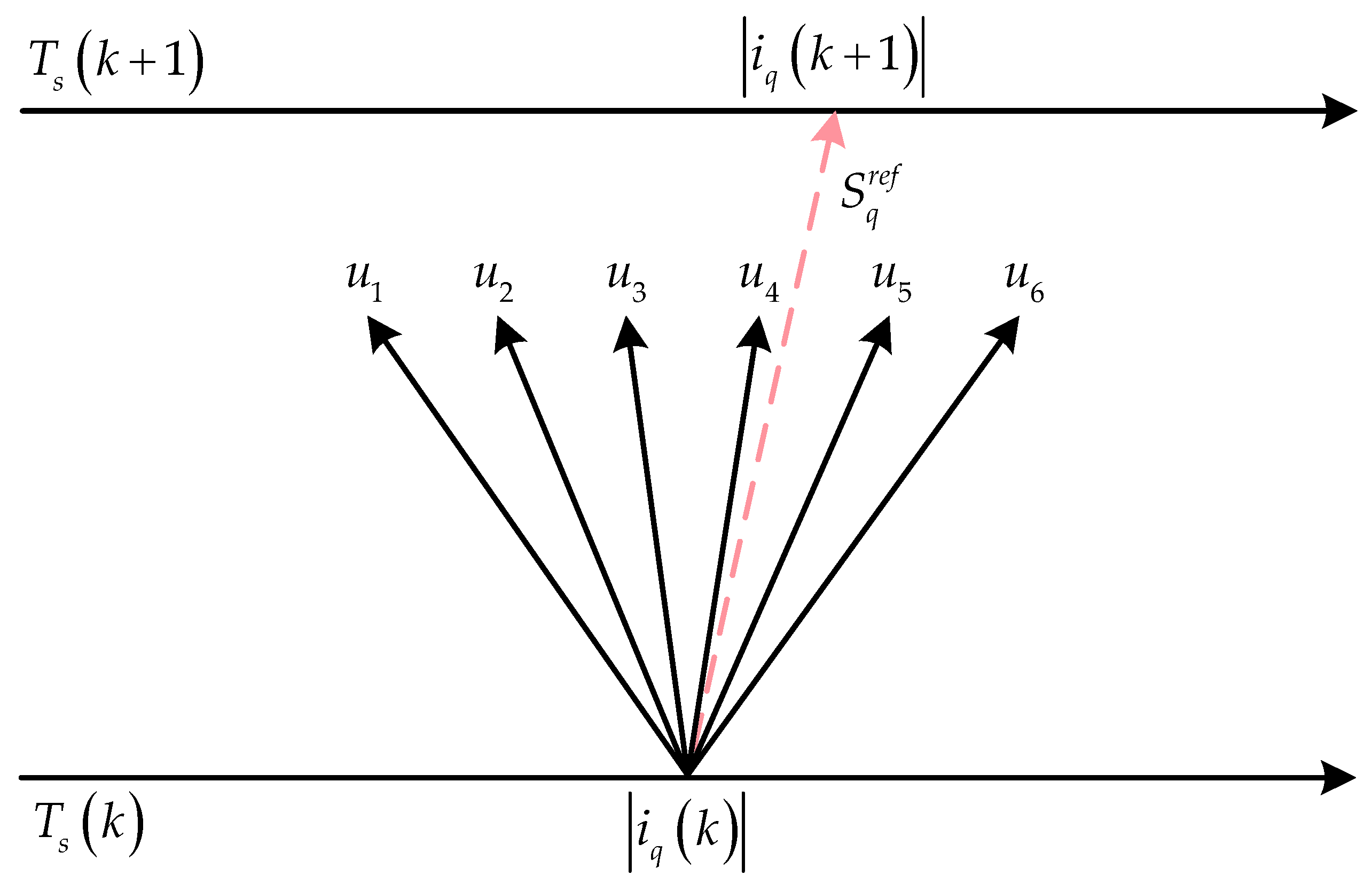
As shown in Figure 6, when $u_{ss-opt2}$ is selected through the comparison mechanism of the q-axis current slope, if the calculated q-axis current reference slope $S_q^{ref}$ is located at the position of the dotted line in the figure, it is evident that the position is closest to the effective voltage vector $u_4$, indicating that at this point, under the action of $u_4$, the action effect of the current slope generated in a single control cycle is closest to the set real-time q-axis current reference slope, and $u_4$ is selected as $u_{ss-opt2}$.

Suppose the q-axis current reference slope $S_q^{ref}$ is precisely in the middle of the q-axis current slopes when two specific effective voltage vectors act. Currently, $u_{ss-opt1}$ is used as a reference to select $u_{ss-opt2}$ according to the principle of minimizing the number of toggle switches. Specifically, suppose $S_q^{ref}$ is in the middle position between $u_4$ and $u_5$, assuming that the selected $u_{ss-opt1}$ is $u_3$. In that case, $u_4$ should be selected as $u_{ss-opt2}$ according to the principle of minimizing the number of toggle switches described above.

The optimal zero vector $u_{ss-opt3}$ under the steady-state operation control method is selected similarly to the optimal zero vector $u_{d-opt3}$ under the dynamic operation control method.

The optimum voltage vector selection table for the motor in steady-state operation is shown in Figure 7:

5. Simulation Results

To verify the effectiveness of the proposed switching current predictive control method based on EMA, the PMSM simulation model is built in the Matlab/Simulink (R2023a) environment. The traditional TV-MPCC method, a direct judgment control method based on the change of q-axis current slope (Q-MPCC), is based on the q-axis current slope operation judgment method of EMA algorithm (EMA-Q-MPCC); these three methods are simulated and compared respectively. The three methods employ the same sample time, control settings, a fixed sampling frequency of 100 kHz, and the $i_d=0$ control technique.

Among these, TV-MPCC employs the dead-beat principle to compute the voltage vector action time and simultaneously accomplishes dead-beat control over the dq-axis current without distinguishing between the motor’s steady-state and dynamic operating conditions. The two fundamental voltage vectors next to each other are the first and second effective voltage vectors. The above analysis shows that when the motor operating conditions change, the slope of the q-axis current will change significantly. The Q-MPCC uses the change of the slope of the q-axis current to determine the current operating conditions of the motor directly and adopts different control strategies under different operating conditions, i.e., the motor adopts the improved DV-MPCC when it is in the dynamic operating condition, and it adopts the improved TV-MPCC when it is in the steady-state operating condition. EMA-Q-MPCC is based on Q-MPCC and introduces the EMA method for determining the operating conditions of the motor.

The simulated PMSM parameters are shown in

Table 3. Parameters of the PMSM.

Parameter	Value	Symbol
Rated Power	3.7	$P$ (kW)
Rated Speed	2000	$N_s$ (rpm)
Rated Voltage	220	$U_n$ (V)
Rated Current	16.5	$I_{ph}$ (A)
Rated Torque	18	$T_{NL}$ (N⋅m)
Pole Pairs	4	$p_n$
Stator Resistance	0.25	$R_s$ ($\mathsf{\Omega }$)
Stator Inductance	1.3	$L_s$ (mH)
Permanent magnet flux linkage	0.1827	${\psi }_f$ (Wb)
Rotational inertia	0.0046	$J$ (kg·m2)

.

5.1. Steady-State Operation Simulation Performance Evaluation

In order to verify the performance of the method proposed in this paper under the steady-state operation condition of the motor, the simulation experiments set the rotational speed of the motor under steady-state operation to 1000 r/min, and the load torque is set to 5 N⋅m.

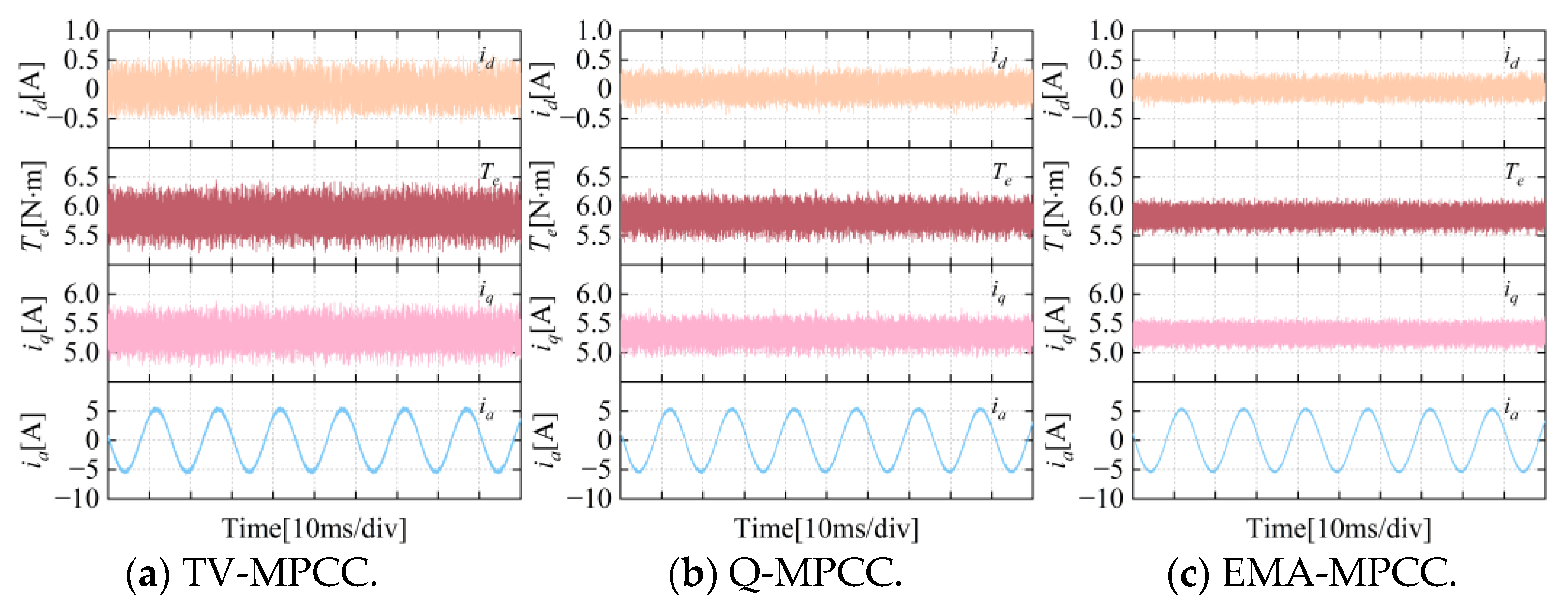
Figure 8 shows the simulated waveforms of the steady-state performance of the motor under the three control methods of TV-MPCC, Q-MPCC, and EMA-Q-MPCC, including the data waveforms of the dq-axis current, torque, and A-phase stator current.

As a statistical index, the standard deviation can effectively reflect the degree of dispersion between the control quantity and its desired value to quantify the control’s accuracy and stability. Therefore, in order to quantitatively evaluate the steady-state performance of the motor, the standard deviation calculation method shown in (27) is used:

$$\sigma =\sqrt{{\displaystyle \frac{1}{N}}{{\displaystyle \sum _{i=1}^N\left(x_i-\frac{1}{N}{\displaystyle \sum _{i=1}^N{x}_i}\right)}}^2}$$

(27)

where $\sigma$ is the standard deviation of d-axis current $i_{d-\sigma }$, the standard deviation of q-axis current $i_{q-\sigma }$, and the standard deviation of torque $T_{e-\sigma }$; N is the number of samples.

Meanwhile, the A-phase stator current is analyzed by Fast Fourier Transform (FFT) to obtain the total harmonic distortion (THD) of the A-phase stator current corresponding to the three methods, and the results are shown in

Table 4. Steady-state performance under three different methods.

Control Methods	${\mathit{i}}_{\mathit{d}-\mathit{\sigma }}$ (A)	${\mathit{i}}_{\mathit{q}-\mathit{\sigma }}$ (A)	${\mathit{T}}_{\mathit{e}-\mathit{\sigma }}$ (N·m)
TV-MPCC	0.22 A	0.23 A	0.25 N·m
Q-MPCC	0.16 A	0.17 A	0.18 N·m
EMA-Q-MPCC	0.12 A	0.13 A	0.14 N·m

:

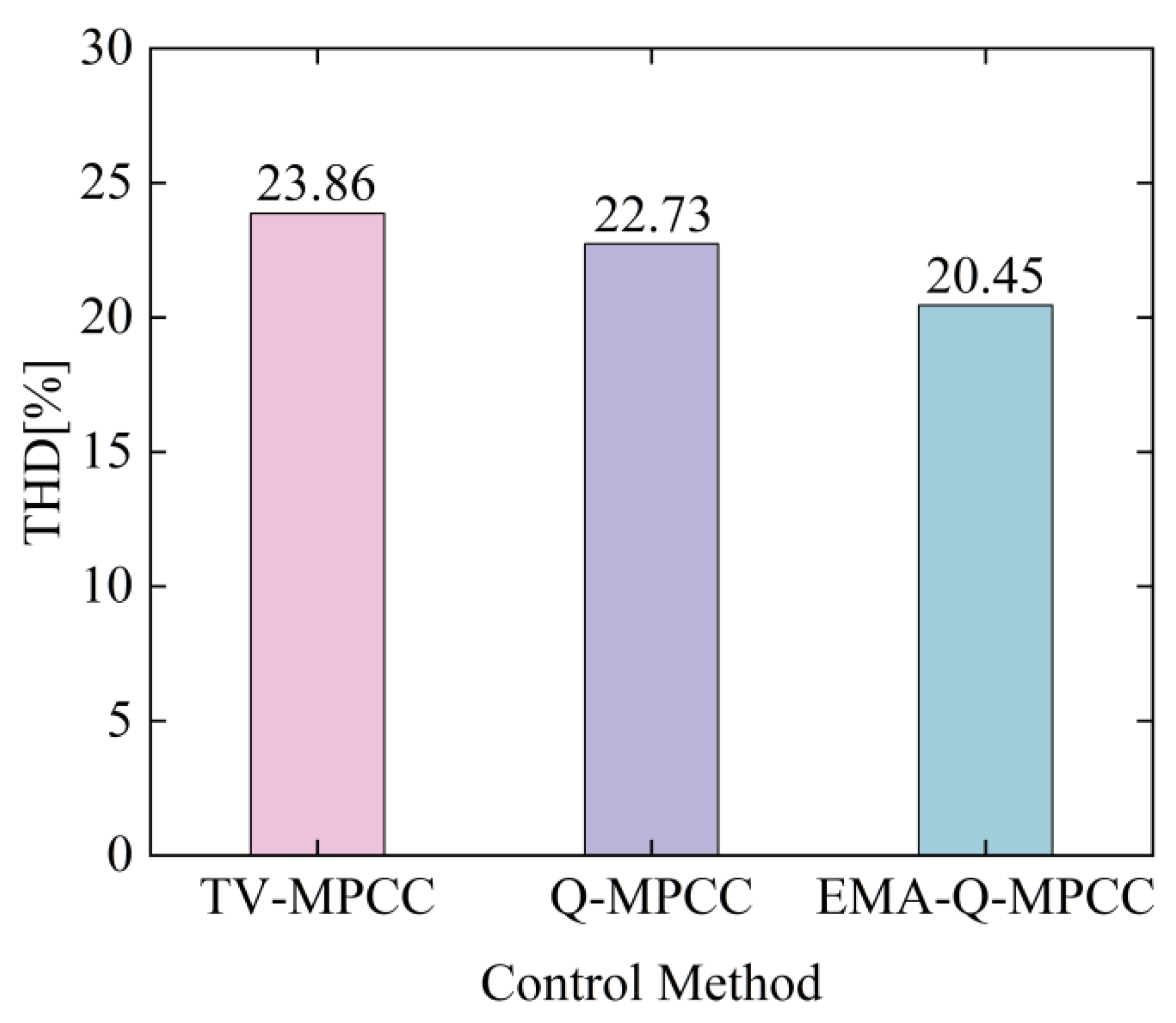
The data in Table 4 show that the EMA-Q-MPCC method has a better suppression effect on dq-axis current and torque ripple than TV-MPCC and Q-MPCC under steady-state operation. Specifically, compared with TV-MPCC, the dq-axis current ripple is reduced by 46.76% and 45.41%, and the torque ripple is reduced by 45.42%. Compared with Q-MPCC, these values are reduced by 27.22%, 25.15%, and 25.13%, respectively. In addition, Figure 9 shows the THD of the A-phase stator current for the three methods, and the proposed method reduces it by 44% and 8% compared to the TV-MPCC and Q-MPCC methods, respectively. This indicates that the proposed method has the best steady-state current performance.

The motor’s performance is examined in further analysis during steady-state operation by applying the same 3 N⋅m loads and setting the reference speed to 500, 700, 900, 1100, 1300, and 1500 r/min, and the same speed is set to 1000 r/min, and the reference load torque is set to 2, 4, 6, 8, 10, 12 N⋅m. Meanwhile, the first-order Eulerian discrete equation in (4) shows that the motor control system under the MPCC method is more sensitive to the inductance parameter. Therefore, to better verify the advantages of the proposed method in terms of robustness, the comparative analysis of motor operation under inductance mismatch is set. The inductance values are set as 0.5, 0.75, 1.0, 1.25, and 1.5 $L_s$ to verify the current and torque performance when the inductance values are varied from as low as 50% to as high as 50%.

Figure 10 and Figure 11 show that the EMA-Q-MPCC has the best current and torque ripple suppression effect at various speeds and load torques. Figure 12 shows that the proposed method has the most minor current and torque ripple amplitude in the case of inductance mismatch, and the suppression of variations in sensitive parameters is better than the previous two methods.

5.2. Performance Evaluation of Dynamic Running Simulation

To validate the performance of the approach provided in this paper under dynamic operating conditions, the reference speed of the motor under no-load conditions is set to be 500 r/min, and the speed is increased abruptly from 500 r/min to 1000 r/min when the simulation experiment is carried out for 0.2 s, and at the same time, in order to verify the motor’s immunity to the load disturbances under the three control methods, the load disturbances are added abruptly for 3 N⋅m load disturbances at 0.4 s.

Figure 13 and Figure 14 show the dynamic changes of speed, torque, and single-phase stator current $i_a$ when the motor speed changes suddenly and when a load is added suddenly. When a sudden load is applied, the three control methods of TV-MPCC, Q-MPCC, and EMA-Q-MPCC can quickly regulate and restore the motor to a stable-state. When the speed is changed abruptly, the dynamic response time to reach the specified reference speed is 12 ms for the first two methods, while the response time for the EMA-MPCC method is 10 ms, which is 16.67% less than the first two methods. Therefore, the proposed method maintains good disturbance resistance and improves the system’s fast response performance.

5.3. Comparison of Computational Burden

To compare the computational complexity of the three control methods, TV-MPCC, Q-MPCC, and EMA-Q-MPCC, the execution times of the three methods are timed and compared using the Tic/Toc function that comes with MATLAB. The test parameter of the simulation is set to be the instantaneous no-load static start of the motor.

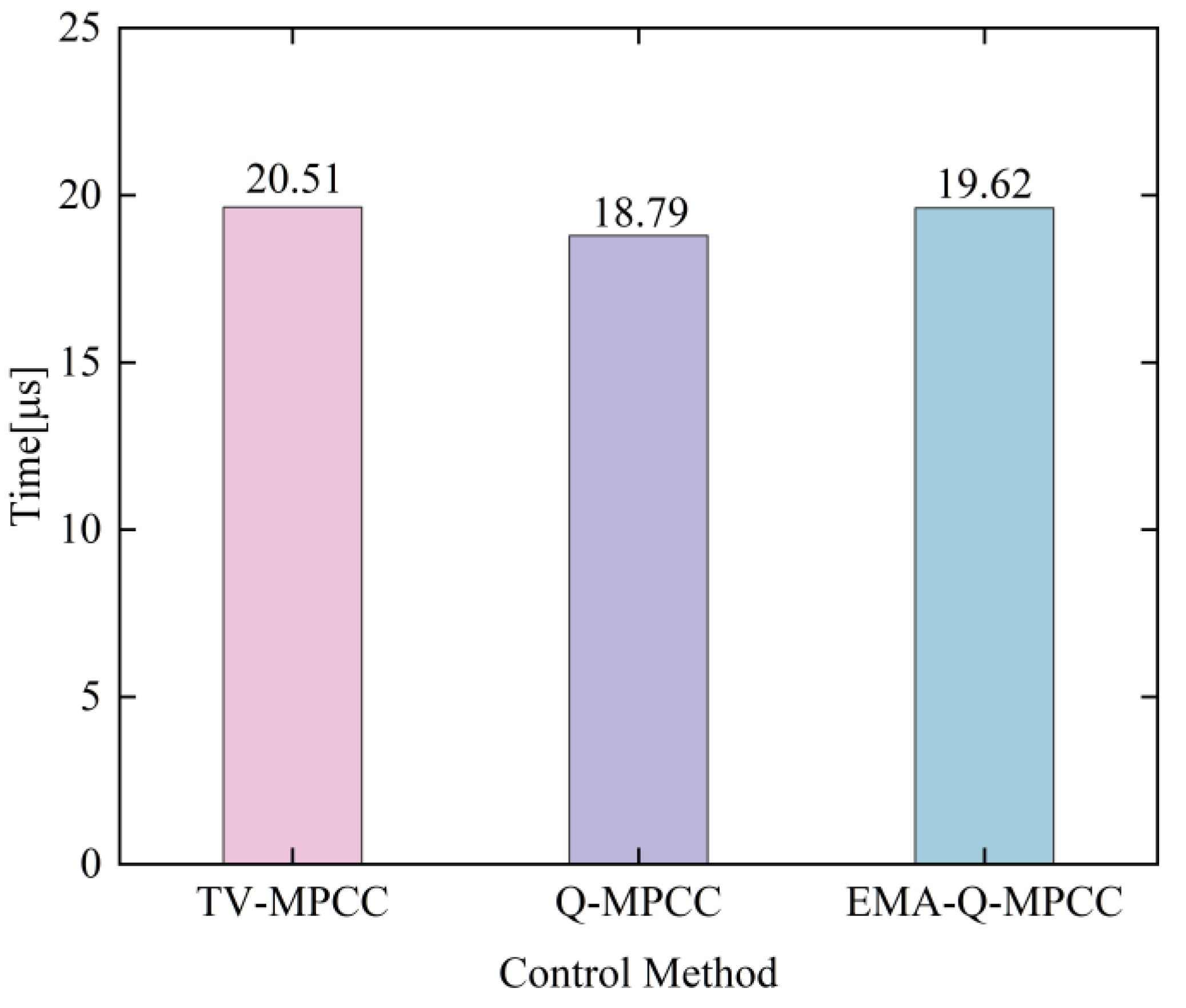
Figure 15 shows the execution time of the three methods by taking the average of 10,000 running times of their test cycles: the average execution time of the three methods, TV-MPCC, Q-MPCC, and EMA-Q-MPCC take 20.51 μs, 18.79 μs, and 19.62 μs, respectively. The proposed method reduces this by 4.34% compared to TV-MPCC. This is mainly because the traditional methods use a value function for optimal search when selecting the optimal voltage vector. In contrast, the proposed method uses the comparison mechanism of q-axis current slopes to select the desired second optimal voltage vector, reducing some of the system’s computational complexity. However, to better discriminate the motor operating conditions, the EMA algorithm is introduced on top of the Q-MPCC method, which leads to an increase in the average execution time of the proposed method compared to it.

6. Experimental Results

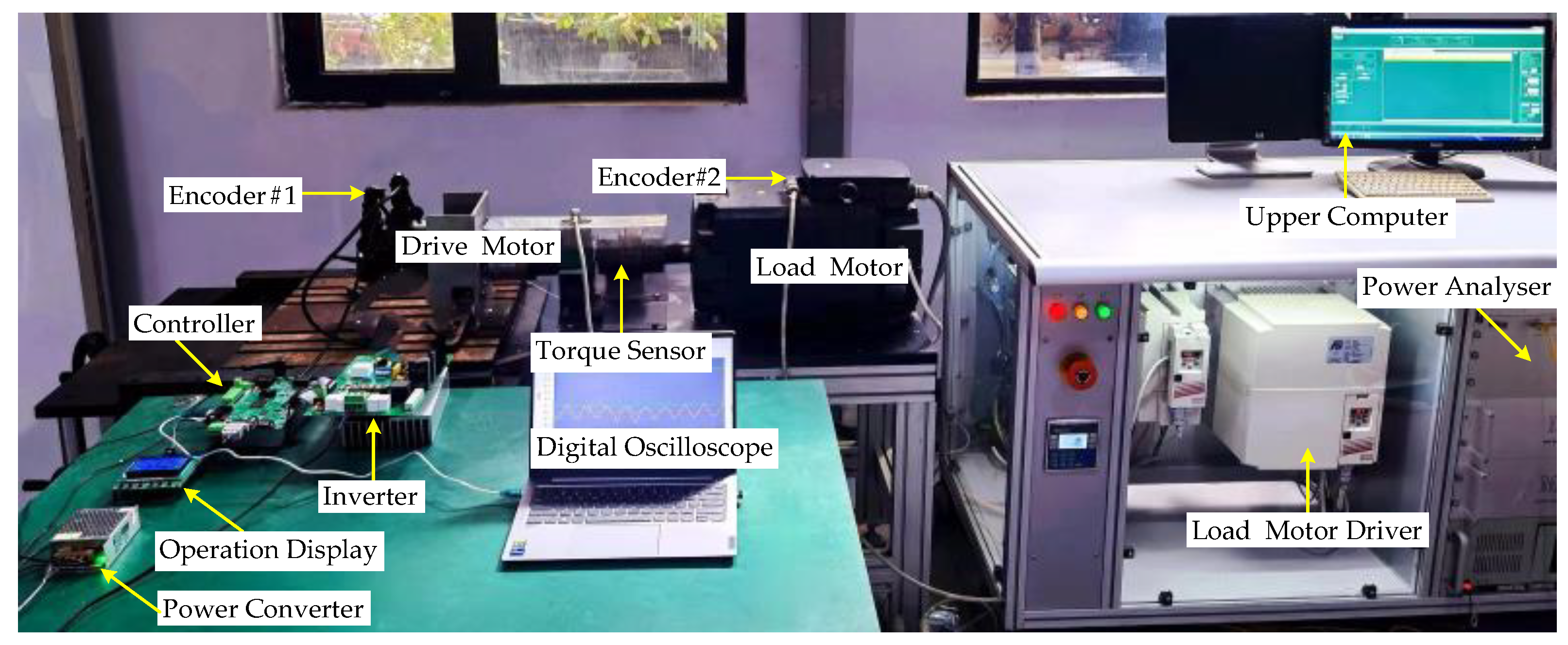
The experimental hardware platform built in this paper is shown in Figure 16. The whole system includes the load motor and drive control module. The upper computer is connected to the load motor through the data transmission line, the load motor is connected to the motor under test through the coupling, and the motor under test is connected to the controller through the encoder output signal interface. The load motor is based on the Regenerative Dynamometer System (RDS) test system, which can be used to test the motor performance by setting different load torques through the host computer. The PMSM-related parameters used in the experiment are the same as those in Table 3, the control frequency of the drive system is set to 10 kHz, and the DC voltage is set to 24 V. During the experiment, the running data of the motors are uploaded in real-time to the PC of the digital oscilloscope through the controller output interface.

6.1. Performance Evaluation of Steady-State Operation Experiments

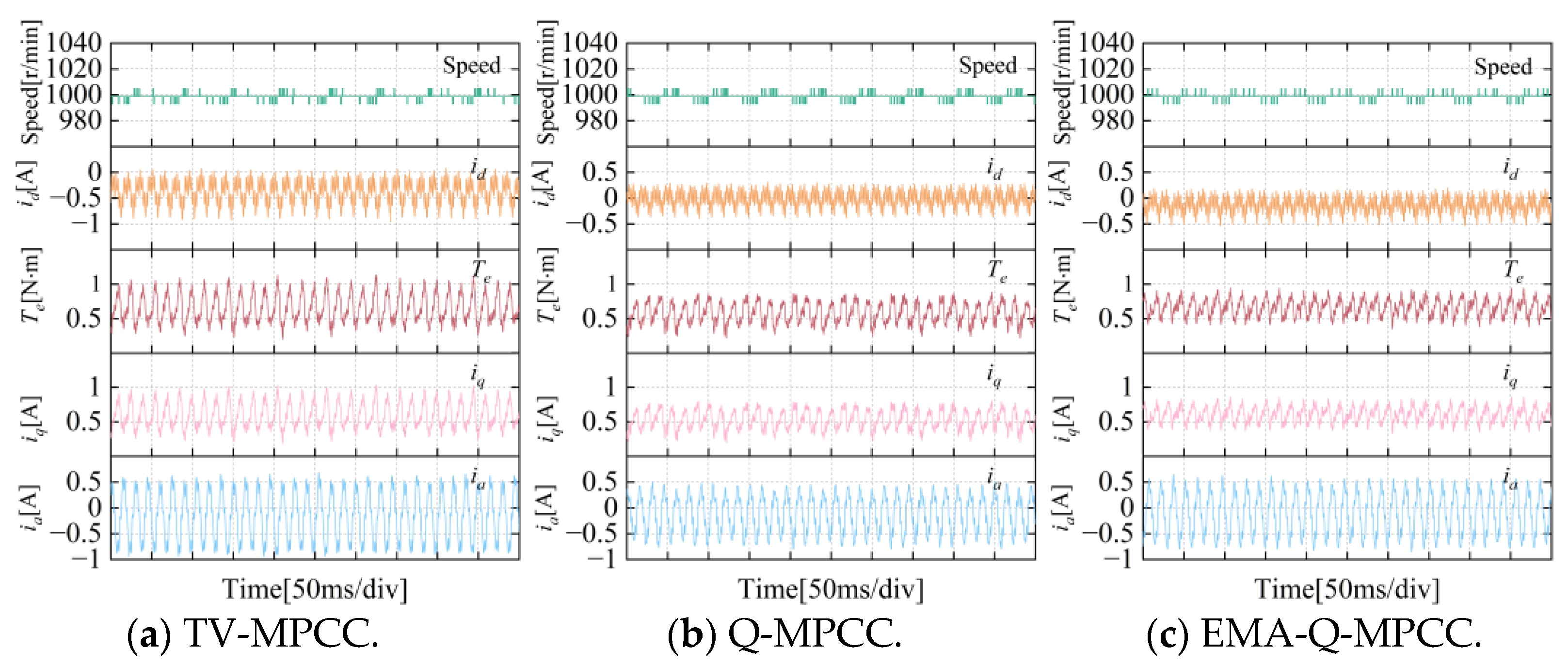
Three control methods, TV-MPCC, Q-MPCC, and EMA-Q-MPCC, are used to evaluate the experimental performance of the PMSM for steady-state operation, respectively. The rotational speed in the experiment is set to 1000 r/min, and the load torque is set to 0.5 N⋅m. Figure 17 shows the experimental waveforms of the steady-state operation of the motor under the three different control methods.

The steady-state performance of the motor under the three methods of TV-MPCC, Q-MPCC, and EMA-Q-MPCC shown in Figure 17 is quantitatively evaluated using the standard deviation equation. At the same time, the A-phase stator current is analyzed by using the FFT, and the THD of the currents corresponding to the three methods is obtained. The results are shown in

Table 5. Experimental performance under three different methods.

Control Methods	${\mathit{i}}_{\mathit{d}-\mathit{\sigma }}$ (A)	${\mathit{i}}_{\mathit{q}-\mathit{\sigma }}$ (A)	${\mathit{T}}_{\mathit{e}-\mathit{\sigma }}$ (N·m)
TV-MPCC	0.22 A	0.19 A	0.21 N·m
Q-MPCC	0.16 A	0.14 A	0.15 N·m
EMA-Q-MPCC	0.15 A	0.11 A	0.12 N·m

:

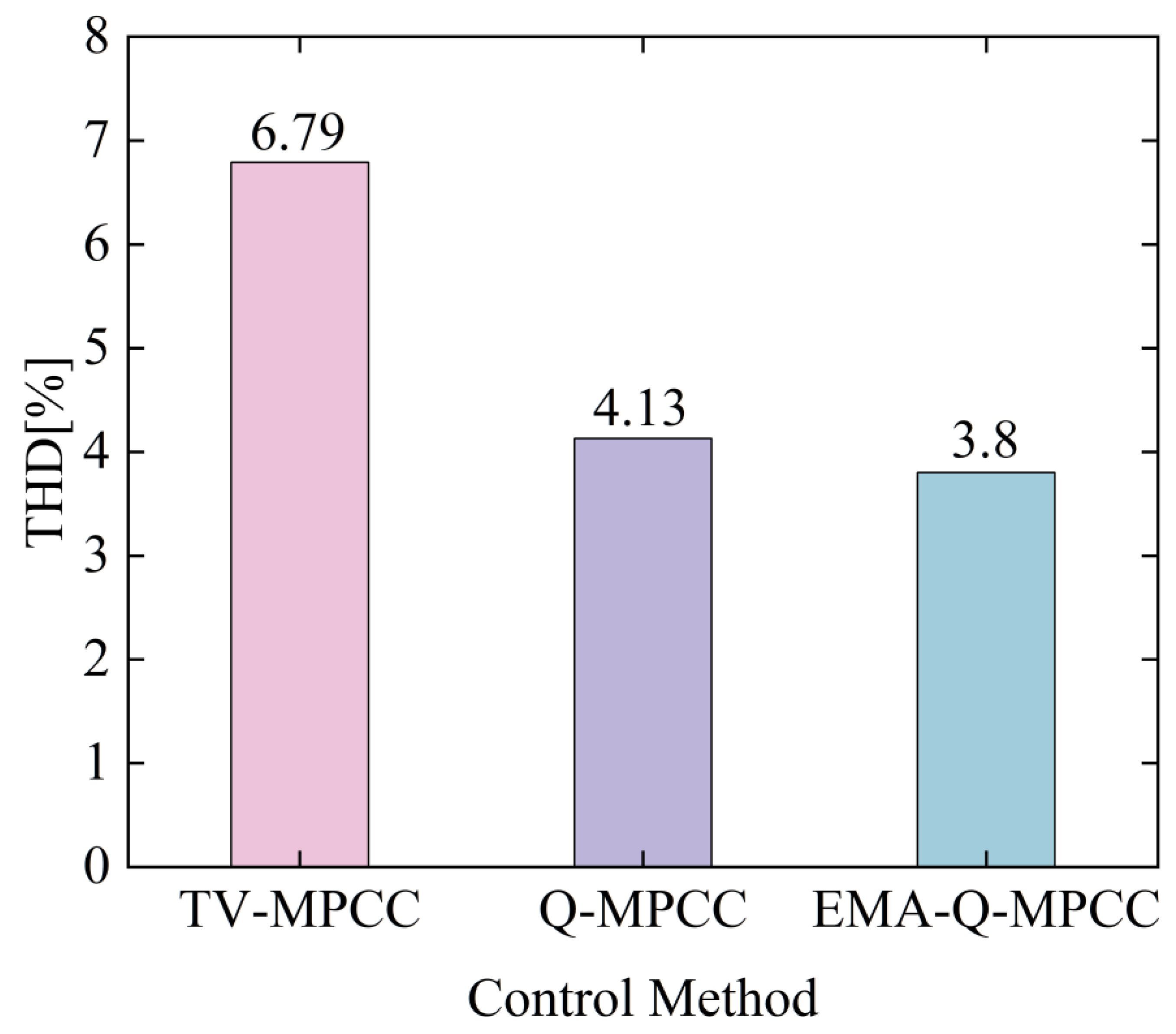
The data in Table 5 show that the EMA-Q-MPCC method has a better suppression effect on dq-axis current and torque ripple than TV-MPCC and Q-MPCC under steady-state experimental operation. Specifically, compared with TV-MPCC, the dq-axis current ripple is reduced by 31.82% and 42.11%, and the torque ripple is reduced by 42.86%. Compared with Q-MPCC, these values are reduced by 6.25%, 21.43%, and 20%, respectively. In addition, Figure 18 shows the THD of the A-phase stator current for the three methods, and the proposed method reduces it by 14.29% and 10.03% compared to the TV-MPCC and Q-MPCC methods, respectively. This indicates that the proposed method has the best steady-state current performance.

6.2. Performance Evaluation of Dynamic Running Experiments

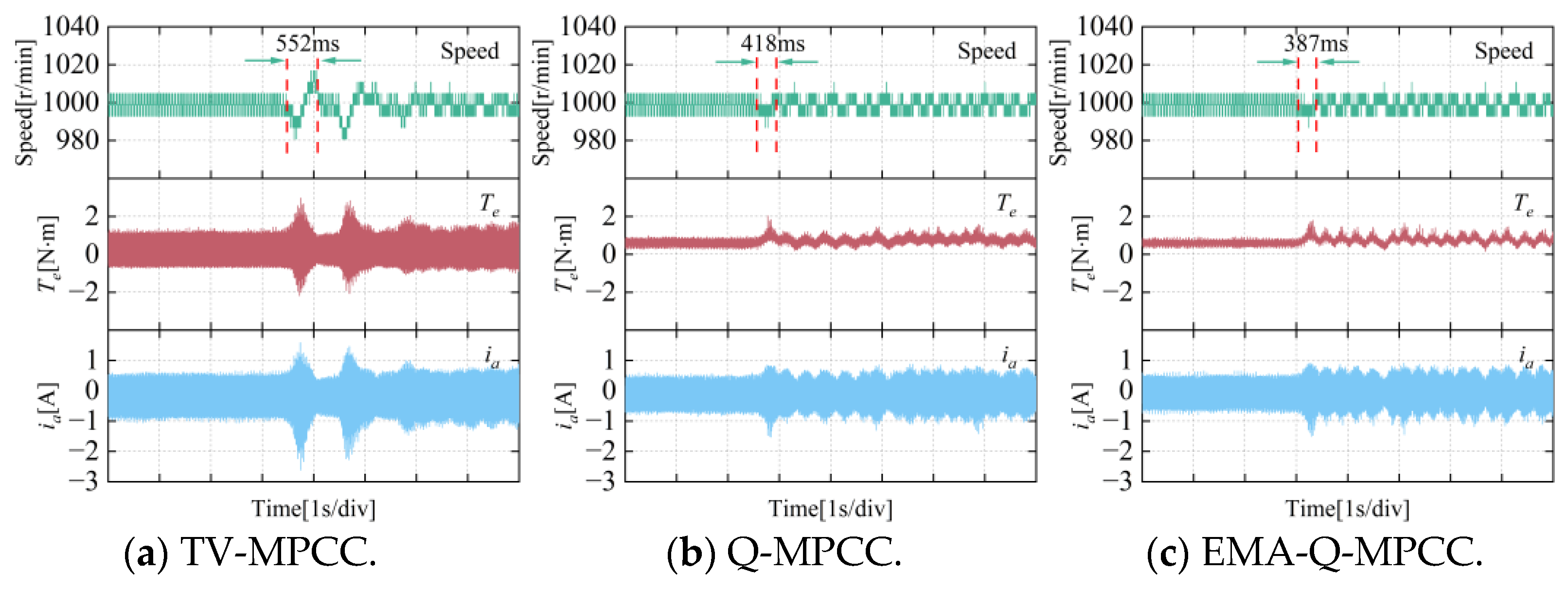
Figure 19 shows the experimental performance evaluation of the PMSM for dynamic operation under three control methods, TV-MPCC, Q-MPCC, and EMA-Q-MPCC, respectively. During the experiment, the motor speed is set to 1000 r/min and a load torque of 2 N·m is added abruptly from the no-load condition. After the sudden addition of 2 N·m load, the fluctuation of the EMA-Q-MPCC method is slight and returns to stability after a short adjustment, and the adjustment time is reduced by 29.89% and 7.42% compared with the previous two methods, which indicates that the proposed method has better adaptability in the face of the load change, and the motor’s dynamic performance is enhanced.

7. Conclusions

This paper proposes a switching current prediction control method based on the Exponential Moving Average (EMA) algorithm to determine the operating conditions of the motor accurately. In the dynamic operation stage, the first and second effective voltage vectors are identical to enhance system efficiency. In the steady-state operation stage, the second voltage vector is selected by comparing the q-axis reference current slope with the q-axis current slopes of all candidate voltage vectors, reducing computational load. Simulation and experimental results demonstrate that the proposed method effectively reduces current and torque ripples, offering high robustness and rapid response, thereby improving the system’s steady-state and dynamic control performance.

The comparison experiments found that the parameter mismatch would affect the motor’s control system. At the same time, reducing the number of switching actions of the switch and improving the system control performance are usually in conflict. Therefore, future research should focus on reducing the dependence on the motor parameters, reducing the switching frequency, and reducing the device’s loss rate to ensure the stability of the control performance.

References

1. Lei, G.; Zhu, J.; Guo, Y.; Liu, C.; Ma, B. A Review of Design Optimization Methods for Electrical Machines. Energies 2017, 10, 1962. [Google Scholar] [CrossRef]
2. Wei, Y.; Young, H.; Ke, D.; Huang, D.; Wang, F.; Rodríguez, J. Adaptive Ultra-Localized Time-Series for Improved Model-Free Predictive Current Control on PMSM Drives. IEEE Trans. Power Electron. 2024, 39, 5155–5165. [Google Scholar] [CrossRef]
3. Wu, Z.; Yang, Z.; Ding, K.; He, G. Transfer Mechanism Analysis of Injected Voltage Harmonic and Its Effect on Current Harmonic Regulation in FOC PMSM. IEEE Trans. Power Electron. 2022, 37, 820–829. [Google Scholar] [CrossRef]
4. Petkar, S.G.; Thippiripati, V.K. A Novel Duty-Controlled DTC of a Surface PMSM Drive with Reduced Torque and Flux Ripples. IEEE Trans. Ind. Electron. 2023, 70, 3373–3383. [Google Scholar] [CrossRef]
5. Yang, J.; Chen, W.-H.; Li, S.; Guo, L.; Yan, Y. Disturbance/Uncertainty Estimation and Attenuation Techniques in PMSM Drives—A Survey. IEEE Trans. Ind. Electron. 2017, 64, 3273–3285. [Google Scholar] [CrossRef]
6. Samad, T.; Bauer, M.; Bortoff, S.; Di Cairano, S.; Fagiano, L.; Odgaard, P.F.; Rhinehart, R.R.; Sánchez-Peña, R.; Serbezov, A.; Ankersen, F.; et al. Industry Engagement with Control Research: Perspective and Messages. Annu. Rev. Control 2020, 49, 1–14. [Google Scholar] [CrossRef]
7. Peng, J.; Yao, M. Overview of Predictive Control Technology for Permanent Magnet Synchronous Motor Systems. Appl. Sci. 2023, 13, 6255. [Google Scholar] [CrossRef]
8. Li, T.; Sun, X.; Lei, G.; Guo, Y.; Yang, Z.; Zhu, J. Finite-Control-Set Model Predictive Control of Permanent Magnet Synchronous Motor Drive Systems—An Overview. IEEE/CAA J. Autom. Sin. 2022, 9, 2087–2105. [Google Scholar] [CrossRef]
9. Wang, F.; He, L.; Rodriguez, J. FPGA-Based Continuous Control Set Model Predictive Current Control for PMSM System Using Multistep Error Tracking Technique. IEEE Trans. Power Electron. 2020, 35, 13455–13464. [Google Scholar] [CrossRef]
10. Ahmed, A.A.; Koh, B.K.; Lee, Y.I. A Comparison of Finite Control Set and Continuous Control Set Model Predictive Control Schemes for Speed Control of Induction Motors. IEEE Trans. Ind. Inform. 2018, 14, 1334–1346. [Google Scholar] [CrossRef]
11. Zheng, Z.; Sun, D. Model Predictive Flux Control with Cost Function-Based Field Weakening Strategy for Permanent Magnet Synchronous Motor. IEEE Trans. Power Electron. 2020, 35, 2151–2159. [Google Scholar] [CrossRef]
12. Wu, X.; Zhang, Y.; Shen, F.; Yang, M.; Wu, T.; Huang, S.; Cui, H. Equivalent Three-Vector-Based Model Predictive Control With Duty-Cycle Reconstruction for PMSM. IEEE Trans. Ind. Electron. 2024, 71, 2395–2404. [Google Scholar] [CrossRef]
13. Gao, J.; Gong, C.; Li, W.; Liu, J. Novel Compensation Strategy for Calculation Delay of Finite Control Set Model Predictive Current Control in PMSM. IEEE Trans. Ind. Electron. 2020, 67, 5816–5819. [Google Scholar] [CrossRef]
14. Sun, Z.; Deng, Y.; Wang, J.; Yang, T.; Wei, Z.; Cao, H. Finite Control Set Model-Free Predictive Current Control of PMSM With Two Voltage Vectors Based on Ultralocal Model. IEEE Trans. Power Electron. 2023, 38, 776–788. [Google Scholar] [CrossRef]
15. Cheng, L.; Jianhui, H.; Jing, S. Dual-Vector Predictive Current Control of Open-End Winding PMSM with Zero-Sequence Current Hysteresis Control. IEEE J. Emerg. Sel. Top. Power Electron. 2022, 10, 184–195. [Google Scholar] [CrossRef]
16. Petkar, S.G.; Eshwar, K.; Thippiripati, V.K. A Modified Model Predictive Current Control of Permanent Magnet Synchronous Motor Drive. IEEE Trans. Ind. Electron. 2021, 68, 1025–1034. [Google Scholar] [CrossRef]
17. Ma, C.; Rodriguez, J.; Garcia, C.; De Belie, F. Integration of Reference Current Slope Based Model-Free Predictive Control in Modulated PMSM Drives. IEEE J. Emerg. Sel. Top. Power Electron. 2023, 11, 1407–1421. [Google Scholar] [CrossRef]
18. Xu, B.; Jiang, Q.; Ji, W.; Ding, S. An Improved Three-Vector-Based Model Predictive Current Control Method for Surface-Mounted PMSM Drives. IEEE Trans. Transport. Electrif. 2022, 8, 4418–4430. [Google Scholar] [CrossRef]
19. Petkar, S.G.; Thippiripati, V.K. Effective Multivector-Operated Predictive Current Control of PMSM Drive with Reduced Torque and Flux Ripple. IEEE Trans. Transp. Electrif. 2023, 9, 2217–2227. [Google Scholar] [CrossRef]
20. Xu, Y.; Ding, X.; Wang, J.; Li, Y. Three-Vector-Based Low-Complexity Model Predictive Current Control with Reduced Steady-State Current Error for Permanent Magnet Synchronous Motor. IET Electr. Power Appl. 2020, 14, 305–315. [Google Scholar] [CrossRef]
21. Zhang, X.; Zhao, Z. Model Predictive Control for PMSM Drives with Variable Dead-Zone Time. IEEE Trans. Power Electron. 2021, 36, 10514–10525. [Google Scholar] [CrossRef]
22. Zhang, X.; Cheng, Y.; Zhao, Z.; Yan, K. Optimized Model Predictive Control with Dead-Time Voltage Vector for PMSM Drives. IEEE Trans. Power Electron. 2021, 36, 3149–3158. [Google Scholar] [CrossRef]
23. Dong, H.; Zhang, Y. A Low-Complexity Double Vector Model Predictive Current Control for Permanent Magnet Synchronous Motors. Energies 2023, 17, 147. [Google Scholar] [CrossRef]
24. Zhang, X.; Li, J. Model Predictive Switching Control for PMSM Drives. IEEE J. Emerg. Sel. Top. Power Electron. 2023, 11, 942–951. [Google Scholar] [CrossRef]
Figure 1. Diagram of circuit topology and basic voltage vector.
Energies 17 03577 g001
Figure 2. Control diagram of the proposed method.
Energies 17 03577 g002
Figure 3. Control diagram for judgment of motor operating conditions.
Energies 17 03577 g003
Figure 4. Control diagram of the steady-state operation control method.
Energies 17 03577 g004
Figure 5. Schematic diagram of the virtual voltage vector coverage.
Energies 17 03577 g005
Figure 6. Diagram of voltage vector selection based on q-axis reference slope.
Energies 17 03577 g006
Figure 7. Diagram of optimal voltage vector selection under the dynamic operational control method.
Energies 17 03577 g007
Figure 8. Steady-state operation diagram of the motor.
Energies 17 03577 g008
Figure 9. Simulation THD of the A-phase current.
Energies 17 03577 g009
Figure 10. Ripple diagrams of three methods under different speeds.
Energies 17 03577 g010
Figure 11. Ripple diagrams of three methods under different torques.
Energies 17 03577 g011
Figure 12. Ripple diagrams of three methods under different inductances.
Energies 17 03577 g012
Figure 13. Dynamic speed variation diagram of three control methods.
Energies 17 03577 g013
Figure 14. Dynamic torque and i a variation diagram of three control methods.
Energies 17 03577 g014
Figure 15. Comparison of computational burden under different methods.
Energies 17 03577 g015
Figure 16. The experimental platform of the PMSM drive system.
Energies 17 03577 g016
Figure 17. Experimental waveforms of steady-state results.
Energies 17 03577 g017
Figure 18. Experimental THD of the A-phase current.
Energies 17 03577 g018
Figure 19. Experimental waveforms of dynamic results.
Energies 17 03577 g019