Article

A Stochastic Model Predictive Control Method for Tie-Line Power Smoothing under Uncertainty

by
Molin An
,
Xueshan Han
* and
Tianguang Lu
School of Electrical Engineering, Shandong University, Jinan 250061, China
*
Author to whom correspondence should be addressed.
Energies 2024, 17(14), 3515; https://doi.org/10.3390/en17143515
Submission received: 5 June 2024 / Revised: 11 July 2024 / Accepted: 15 July 2024 / Published: 17 July 2024

Abstract

:
With the high proportion of distributed energy resource (DER) access in the distributed network, the tie-line power should be controlled and smoothed to minimize power flow fluctuations due to the uncertainty of DER. In this paper, a stochastic model predictive control (SMPC) method is proposed for tie-line power smoothing using a novel data-driven linear power flow (LPF) model that enhances efficiency by updating parameters online instead of retraining. The scenario method is then employed to simplify the objective function and chance constraints. The stability of the proposed model is demonstrated theoretically, and the performance analysis indicates positive results. In the one-day case study, the mean relative error is only 1.1%, with upper and lower quartiles of 1.4% and 0.2%, respectively, which demonstrates the superiority of the proposed method.

1. Introduction

The prevalence of DER, including photovoltaic (PV), wind turbine (WT) and energy storage (ES), has become a significant element of power systems [1]. Furthermore, DER operates intermittently, stochastically, and with fluctuations, creating new challenges for tie-line power management [2]. To manage the high proportion of DER access, operators must control the tie-line power to realize smoothing by following a given reference value, which can help ensure the safety and consider the economic factors of the loads. Therefore, tie-line power control and smoothing are being increasingly studied.
Numerous studies have explored tie-line power control and smoothing for various objectives in different circumstances. The authors of [3] proposed a multi-agent-based distributed optimal tie-line power flow control strategy that can maintain a schedule in the presence of any disturbance. The authors of [4] examined wide-area control architecture and an output regulation approach in combination with LQ optimal control to effectively smooth short-term tie-line power fluctuations. The authors of [5] presented a strategy for smoothing external tie-line power fluctuations in a new urban power grid. To minimize the tie-line power flow, a superconducting magnetic energy storage (SMES) method with fuzzy logic control and optimized fuzzy logic control was investigated in [6]. A flat tie-line power control for WT and PV energy in a grid-connected microgrid (MG) supported by ES was proposed in [7]. A droop control strategy was developed to maintain constant tie-line power suitable for the DC–MG by coordinating the designs for the droop control characteristics of the generators, ES, grid-connected inverter, and dead band [8]. The authors of [9] proposed a demand-side management method with game theory to smooth the tie-line power of MGs. A unifying hierarchical control scheme based on distributed communication was proposed in [10]; in this scheme, a pinning control strategy is unified with the distributed optimization and average voltage regulation control loops. The researchers proposed an optimal coordination control strategy for hybrid ES systems based on continuous-state constraints to provide an efficient tie-line smoothing service [11]. The authors of [12] proposed a bi-level optimization model to control tie-line power based on an MG aggregator to manage trading power between the multi-MG and main grid. An interlink inverter control method was further proposed to provide a constant tie-line smoothing service in a grid-connected residential MG to mitigate the fluctuating nature of renewable power generation and load demand [13]. The authors of [14] developed a multi-time-scale tie-line energy and reserve allocation model that features two levels in the control structure, two time scales in the dispatch sequence, and multiple areas integrated within the WT as scheduling objects.
Table 1 provides a comparison between the above literature and the proposed method. Some studies did not study the voltage control. However, we consider this element in our research, as voltage control is critical to ensure safe operation. With the high proportion of DER access in the distributed network, ES becomes increasingly significant, but some studies have not investigated relevant control strategies, e.g., [3,4,9,14]. The present study considers ES to utilize the flexibility and controllability of this element. The uncertainty [15] and time-coupling constraints [16] of DER must be considered. However, most studies focused on short time scales or real-time control, with few studies considering uncertainty, such as [5,9,12,14]. In addition, the power flow is nonlinear and complex, but only the authors of [4,12,14] applied the LPF model to improve efficiency. The above studies used optimization, game theory, and control theory, respectively. Among all studies using control theory, only [4,11,13] utilized a modern control alternative, while the remainder used the classical control method. All of the objectives in Table 1 are considered in this paper, and an SMPC model is proposed to control and smooth the tie-line power. The following factors are considered in this work.
The MPC model has been widely applied in power system operation, including for optimal scheduling [17], voltage control [18], and energy management [19]. However, a high proportion of DER access leads to randomness [20], the uncertainty of which should be considered [21]. By combining stochastic optimization with the standard MPC method [22], SMPC can effectively operate under chance constraints and has achieved good results in energy management [23] and optimal dispatching [24] due to the development of forecasting and measurement technology. Therefore, we use SMPC to realize tie-line power smoothing and account for the related uncertainty. By setting a reasonable objective function, this method can also satisfy the corresponding economic indicators, thereby achieving a win–win situation offering both accuracy and low economic cost.
The state equation represented by the power flow is the cornerstone of the SMPC model. Therefore, the complexity and efficiency of the SMPC model are determined by the form of the power flow. The LPF model is widely used for voltage control [25], optimal scheduling [26], economic operation [27], and service restoration [28] due to its simplicity and speed. There are various methods to obtain the LPF model, but it iscrucial to select one that would be appropriate for this study. LPF models are classified into two categories: traditional model-driven and novel data-driven [29] methods. Over the past decade, LPF models have evolved from the former [30] to the latter [31]. Notably, data-driven models are not reliant on the power system’s structure [32]. Consequently, we selected a data-driven model for this paper. However, this type of model has strict requirements for data quality [33] and measurement accuracy [34]. Additionally, data-driven LPF models often require retraining during use, and their generalization ability (the ability to maintain accuracy with new data over time without retraining) is weak [35]. In conclusion, an ideal LPF model should possess the following characteristics: accuracy, speed, strong generalization ability, and a low data burden. Consequently, a new, superior LPF model is applied in this work to achieve fast optimization for tie-line smoothing. This measure can greatly reduce the complexity and improve efficiency.
To achieve the above-mentioned objectives, an online updated LPF model is first used to improve efficiency. Then, we derive an MPC model for tie-line power smoothing. Finally, the SMPC model is established to account for uncertainty, and the scenario method is adopted to simplify the model.

2. Methods

2.1. LPF Model

Regression learning is performed on historical data to obtain the LPF model. The SMPC model uses the incremental LPF model as the state equation ( P 0 ) and the normal form as the constraint ( U i ). The LPF model is derived through several steps.
For simplicity, the following definitions are used:
P = ( p 1 , p 2 , , p n ) T
Q = ( q 1 , q 2 , , q n ) T
P 2 = ( p 1 2 , p 2 2 , , p n 2 ) T
Q 2 = ( q 1 2 , q 2 2 , , q n 2 ) T .
The tie-line power model trained after regression learning is
P 0 ( k ) = R P 0 q u a P 2 ( k ) + X P 0 q u a Q 2 ( k ) + R P 0 l i n P ( k ) + X P 0 l i n Q ( k ) + A P 0 c o n
where the superscript is the coefficient name, and R , X , and A are unknown parameters before training.
The above model is trained through regression learning using the historical data from P 0 , P , and Q to obtain R , X , and A . However, the model trained after regression learning is quadratic. The Taylor expansion is applied to obtain the LPF model. After the Taylor expansion, the following incremental LPF model is derived:
P 0 ( k + 1 ) = P 0 k + R P 0 i n c Δ P ( k ) + X P 0 i n c Δ Q ( k )
  R P 0 i n c = 2 R P 0 q u a P ( k ) T + R P 0 l i n
X P 0 i n c = 2 X P 0 q u a Q ( k ) T + X P 0 l i n
where represents the Hadamard Product.
The normal form for the voltage constraint can be derived in the same way:
U j ( k + 1 ) = R U j n o r P ( k ) + X U j n o r Q ( k ) + A U j n o r
  R U j n o r = 2 R U j q u a P ( k ) T + R U j l i n
X U j n o r = 2 X U j q u a Q ( k ) T + X U j l i n
A U j n o r = U j ( k ) 2 R U j q u a P 2 ( k ) R U j l i n P ( k ) 2 X U j q u a Q 2 ( k ) X U j l i n Q ( k ) .
The full derivation process and training approach is detailed in [36], which also elaborates on the principles and reasons for choosing a quadratic model for training and applying the Taylor expansion to obtain the LPF model.

2.2. Derivation of the SMPC Model

The above linear tie-line power model is simplified as follows:
P 0 ( k + 1 ) = P 0 ( k ) + B ( k ) u ( k )
u ( k ) = ( Δ P ( k ) T , Δ Q ( k ) T ) T
B ( k ) = ( R P 0 i n c , X P 0 i n c ) .
The reference value after time k is
P 0 r e f = ( P 0 r e f ( k + 1 ) , P 0 r e f ( k + 2 ) , , P 0 r e f ( k + N ) ) T .
The calculated value after time k is
P 0 ¯ ( k + 1 ) = ( P 0 ( k + 1 | k ) , P 0 ( k + 2 | k ) , , P 0 ( k + N | k ) ) T .
The calculated control command is
u ¯ ( k ) = ( u ( k ) , u ( k + 1 | k ) , , u ( k + N 1 | k ) ) T .
Then, we derive the following model:
P 0 ¯ ( k + 1 ) = M P 0 ( k ) + C ( k ) u ¯ ( k )
M ( k ) = ( 1 , 1 , , 1 ) 1 × N T
C ( k ) = B ( k ) 0 0 0 B ( k ) B ( k + 1 ) 0 0 B ( k ) B ( k + 1 ) B ( k + 2 ) 0 0 B ( k ) B ( k + 1 ) B ( k + 2 ) B ( k + N 1 ) .
The objective function for the next N times after time k is constructed as
J ( k ) = ( P 0 ¯ ( k + 1 ) P 0 r e f ) T Q ( P 0 ¯ ( k + 1 ) P 0 r e f ) + u ¯ ( k ) T R u ¯ ( k ) .
Q and R are coefficient matrices:
Q = q × I N , R = r × I N
where p and q represent the weights. The objective function is used to minimize the tie-line power discrepancy with minimal adjustments to the user power cost.
For convenience, the simplified standard form is derived as follows:
J ( k ) = ( P 0 ¯ ( k + 1 ) P 0 r e f ) T Q ( P 0 ¯ ( k + 1 ) P 0 r e f ) + u ¯ ( k ) T R u ¯ ( k ) = ( M P 0 ( k ) + C ( k ) u ¯ ( k ) P 0 r e f ) T Q ( M P 0 ( k ) + C ( k ) u ¯ ( k ) P 0 r e f ) + u ¯ ( k ) T R u ¯ ( k ) = ( e ( k ) + C ( k ) u ¯ ( k ) ) T Q ( e ( k ) + C ( k ) u ¯ ( k ) ) + u ¯ ( k ) T R u ¯ ( k ) = e ( k ) T Q e ( k ) + u ¯ ( k ) T C ( k ) T Q C ( k ) u ¯ ( k ) + 2 e ( k ) T Q C ( k ) u ¯ ( k ) + u ¯ ( k ) T R u ¯ ( k ) = u ¯ ( k ) T ( C ( k ) T Q C ( k ) + R ) u ¯ ( k ) + 2 e ( k ) T Q C ( k ) u ¯ ( k ) + e ( k ) T Q e ( k ) .
The error matrix is:
e ( k ) = M P 0 ( k ) P 0 r e f .
J ( k ) is converted into a standard form:
J ( k ) = 1 2 u ¯ ( k ) T H ( k ) u ¯ ( k ) + f ( k ) u ¯ ( k ) + d ( k )
H ( k ) = 2 ( C ( k ) T Q C ( k ) + R )
f ( k ) = 2 e ( k ) T Q C ( k )
d ( k ) = e ( k ) T Q e ( k ) .
The model also includes a terminal equality constraint:
s . t .   P 0 ( k + T ) P 0 r e f ( k + T ) = 0 .
PV, ES, and flexible loads satisfy the following constraints, which can be derived using any linearization method:
Z i k = { ( p i k , q i k ) | Ω 1 p i k + Ω 2 q i k c i k }
where Ω represents a set of linear parameter vectors, and c represents the capacity.
In addition, the constraints of ES include the following:
E i , k + 1 E S S = E i , k E S S + η c h a P i , k c h a Δ t 1 η d i s P i , k d i s Δ t
P i , k E S S = P i , k d i s P i , k c h a
0 P i , k c h a μ i , k c h a P max E S S
0 P i , k d i s μ i , k d i s P min E S S
μ i , k c h a + μ i , k d i s 1
μ i , k c h a , μ i , k d i s 0 , 1
E min E S S E i , k E S S E max E S S
where E is the capacity of ES, P is the power, μ is the 0–1 variable indicating charge and discharge, η is the efficiency of charge and discharge, dis represents discharge, cha represents charge, and Δ t is the time interval.
The adjustable range is indicated by Δ Z i . The adjustment of the node after receiving an instruction is
Δ Z i , a d j = u ( k ) ( Z i , b e f o r e ( k + 1 ) Z i , a f t e r ( k ) )
where the subscripts indicate the values before and after adjustment.
The SMPC model is then established as follows:
min   E k [ J ( k ) ]
s . t .   P 0 ¯ ( k + 1 ) = M P 0 ( k ) + C ( k ) u ¯ ( k )
U j ( k + 1 ) = R U j n o r P ( k ) + X U j n o r Q ( k ) + A U j n o r
Δ Z i , a d j Δ Z i       i = 1 , 2 , , n
P U j ( k ) U max 0 1 ε       j = 1 , 2 , , n
P U min U j ( k ) 0 1 ε       j = 1 , 2 , , n
Required to satisfy constraints in Equations (30)–(39)
where E represents the mean of the objective function, and P represents the constraints satisfied with a certain probability. The uncertainty mainly arises from inaccurate predictions of loads or DER influenced by energy prices, weather conditions, and energy demands [37]. We assume that the actual value follows a normal distribution and that the mean is the predicted value with a variance of 0.002.
Finally, the proposed model is uniformly asymptotically stable and able to realize tie-line smoothing, which is demonstrated as follows.
At time k , we choose the Lyapunov function:
V ( k ) = J * ( k ) = i = 1 N P 0 ( k + i | k ) P 0 r e f ( k + i ) Q 2 + i = 0 N 1 u ( k + i ) R 2 .
At time k + 1 , the objective function corresponding to a feasible solution is
J   ( k + 1 ) = i = 1 N P 0 ( k + 1 + i | k ) P 0 r e f ( k + 1 + i ) Q 2 + i = 0 N 1 u ( k + 1 + i ) R 2 = i = 2 N P 0 ( k + i | k ) P 0 r e f ( k + i ) Q 2 + i = 1 N 1 u ( k + i ) R 2 = i = 1 N P 0 ( k + i | k ) P 0 r e f ( k + i ) Q 2 + i = 0 N 1 u ( k + i ) R 2 P 0 * ( k + 1 | k ) P 0 r e f ( k + 1 ) Q 2 u * ( k ) R 2 = J * ( k ) P 0 * ( k + 1 | k ) P 0 r e f ( k + 1 ) Q 2 u * ( k ) R 2 .
Then, we can deduce that
V ( k + 1 ) V ( k ) = J *   ( k + 1 ) J * ( k ) J   ( k + 1 ) J * ( k ) P 0 * ( k + 1 | k ) P 0 r e f ( k + 1 ) Q 2 u * ( k ) R 2 0
V ( 0 ) = 0
P 0 ( k + i ) 0     i = 1 , 2 , N ,     V ( k ) 0 .
Therefore, the SMPC model is uniformly asymptotically stable according to control theory.

2.3. Simplification of the Objective Function and Chance Constraints

In the above SMPC model, uncertainty creates complexity when calculating the expectation of the objective function and the chance constraints, thereby reducing calculation efficiency. For this reason, the following methods are used to simplify and accelerate the calculations.
Suppose that the expected value of J ( x ) with uncertainty is
E X [ J ( X ) ] = J ( x ) p ( x ) d x
where p ( x ) is a probability distribution.
In many cases, this form of integration is impossible or difficult to calculate. In some cases, the probability density function may be unknown. However, this value can be calculated as follows. Suppose there is another distribution q ( x ) called the proposal distribution, based on which the above equation can be expressed as
E ^ X [ J ( X ) ] = 1 N i = 1 N γ i J ( x ( i ) )
γ i = p ( x ( i ) ) q ( x ( i ) )
where γ i is the weight coefficient.
The following conclusion is then deduced [38] as follows:
E ^ X [ J ( X ) ] E X [ J ( X ) ]     a s     N .
Therefore, an expectation that is challenging to calculate is approximated as a sum over a finite number of scenarios. In the simplest case, we can set p ( x ) = q ( x ) and sample directly from the target distribution, which is known as fair sampling.
Uncertainty also has an impact on the constraints and generally appears as chance constraints in SMPC problems:
min l ( α )
s . t .     P ω φ ( α , ω ) 0 1 ε
where l is the objective function, α is the optimization variable, ω is the parameter with uncertainty following the probability distribution P ω , and the parameter ε ( 0 , 1 ) .
The scenario method is used for calculations with the following steps.
(a) Solve the optimization problem
min l ( α )
s . t .     φ ( α , ω i ) 0     i 1 , 2 , , N
and store the solution, which is denoted as S.
(b) Let i run over 1 , 2 , , N and find the active constraints caused by S:
φ ( α S O L , ω i ) = 0 .
These indexes are marked as i 1 , i 2 , , i q .
(c) Find the constraints violated by S:
φ ( α S O L , ω i ) > 0 .
These indexes are marked as j 1 , j 2 , , j l (step c is skipped for the first round).
If L is greater than or equal to [ ε N ] , where ε is a chosen parameter that satisfies 0 ε < ε , then break the algorithm and return S.
(d) For k = 1 , 2 , , q :
Solve the optimization problem
min l ( α )
s . t .     φ ( α , ω i ) 0     i 1 , 2 , , N \ i k , j 1 , j 2 , , j l .
If the calculated objective function is better than S, then the last solution is stored as a new S. End For.
(e) Go to (b).
There are many ways to choose the sampling number N [39,40,41,42]. For this purpose, we adopt the following method:
Denote r as the dimension of the optimization variable.
If N satisfies
ε N + r ε N i = 0 ε N + r N i ε i ( 1 ε ) N i β ,
then the results of the scenario method are satisfied at a confidence level of 1 β .
Using an approximate calculation and derivation [43], this value is simplified as
N 2 ε ln 1 β + r .
The operation of the proposed method is elaborated as follows (see Figure 1):
(1) The operator predicts the load and PV curves for the day. The operator obtains the daily tie-line power schedule in advance as a reference value and trains the LPF model via regression learning.
(2) The operator uses the scenario method to simplify the objective function with uncertainty and converts the chance constraints into linear constraints.
(3) The operator calculates the SMPC model and obtains the result at time k . Only the control instruction corresponding to time k + 1 is selected and sent to users.
(4) After receiving the instructions at time k + 1 , users complete the adjustments.
(5) According to the latest measurement data, the operator updates the SMPC model with the value at time k + 1 .
(6) Return to step 2.

3. Results

3.1. Data Preparation

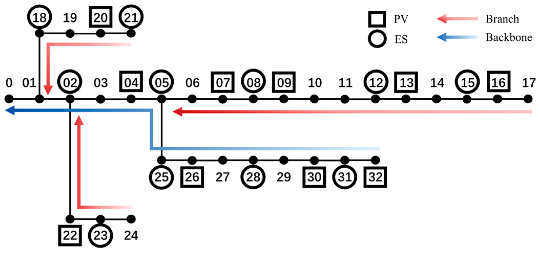
Figure 2 presents the network structure. Based on the parameters of the IEEE 33-node model, the actual load and PV data are used for the LPF model comparison, and ES is used for the SMPC analysis. The blue and red arrows are used for subsequent analysis which will be explained later.
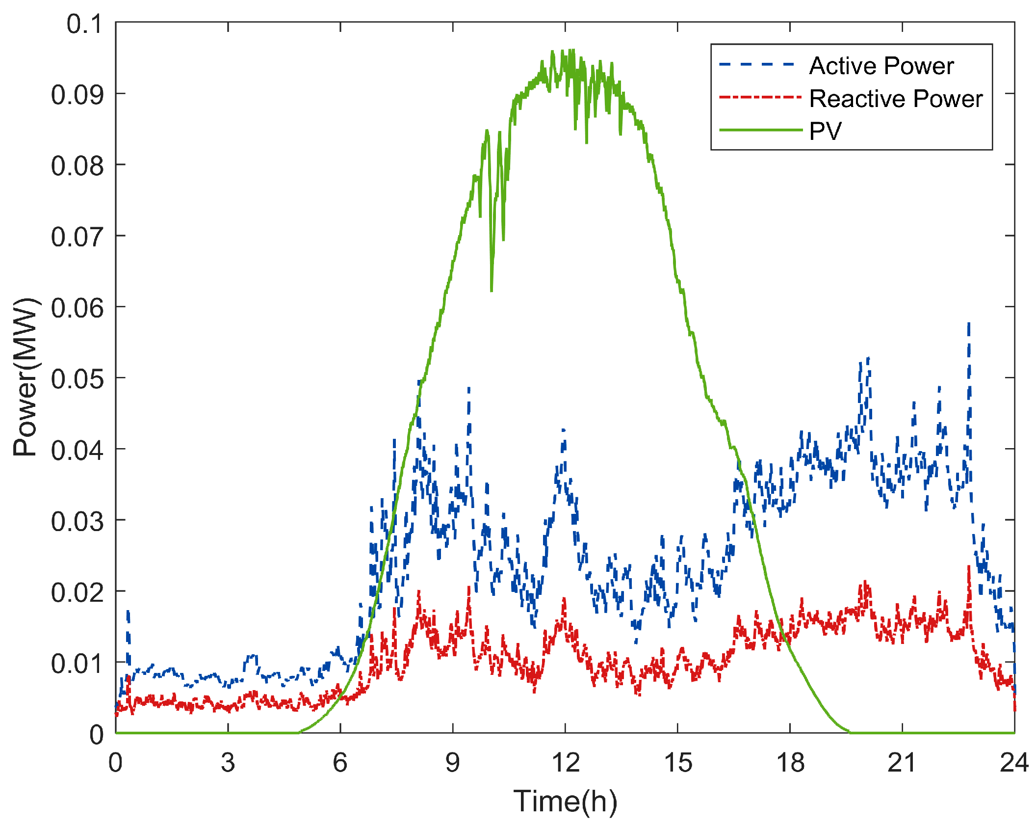
Figure 3 presents the typical loads and PV over a day. We choose the load data and PV data of node 9 as an example. The variation of the load in the rest of the nodes during the day is approximated based on the value of each node. The PV power profiles of the other users are similar to the typical curves because they are affected by the intensity of sunlight, and the weather conditions are consistent within this network.
Based on the load and PV data shown in Figure 3 and the predicted data from other nodes, the dispatching operator calculates the predicted tie-line power values for the next day. The related analysis of the reference value of the tie-line power is shown in Figure 4. Here, the blue line represents the day-ahead prediction of the tie-line power. The prediction data, however, are inaccurate and lead to uncertainties and errors, which are further illustrated in Figure 5. Consequently, the treatment of uncertainty in Section 2.3 is crucial. On the other hand, the fluctuations caused by this uncertainty reinforce the need to use a reasonable calculation for tie-line power control to achieve synergistic cooperation between PV and ES. For this reason, we selected the SMPC method.
The red line represents the reference value of the tie-line power, which includes a series of platforms and drop-offs. In the platform area, the tie-line power is guaranteed to maintain the constant reference value for several hours, effectively creating a network of controlled power (constant but not zero). In climbing or descending drop regions, the tie-line power will increase or decrease at a constant rate, while the predicted values of the same time period will fluctuate considerably. We hope that the proposed method will not only ensure sustained tie-line power value for a defined period, but also facilitate constant-rate adjustments during periods of significant power fluctuation.
Generally, the reference value is set by the dispatching operator based on the predictions of the distribution network and instructions from the higher-level grid. It remains common to set the reference value to a curve, but we artificially set it to a fold line in this study. Using a fold line for the reference value creates significant difficulties compared to setting it as a curve closer to the predicted value, as illustrated by the green curve in Figure 4. Since the ES capacity is time-coupled, it is necessary to optimize this feature over a long time scale to provide an operational strategy, which represents a benefit of using SMPC for optimization. Green curves that are closer to the predicted values and require fewer ES operations will reduce the difficulty of the calculation. For this reason, the reference value is set as the fold line, which is undoubtedly more extraordinary, to demonstrate the superiority of the proposed SMPC model with a more challenging situation. In addition, it brings other advantages. Firstly, the fold line can ensure the constant power of the tie-line in some time periods, which is more stable and flat compared to the curve, and will bring significant convenience to the dispatching. Secondly, this extraordinary and challenging condition also paves the way for performance analysis. In this case, we would like to validate the good performance of the proposed method to fully demonstrate its superiority under different conditions, especially in such extraordinary and challenging conditions. The stability, which was demonstrated in Section 2.2, is further clarified and demonstrated with this case study in the next performance analysis.
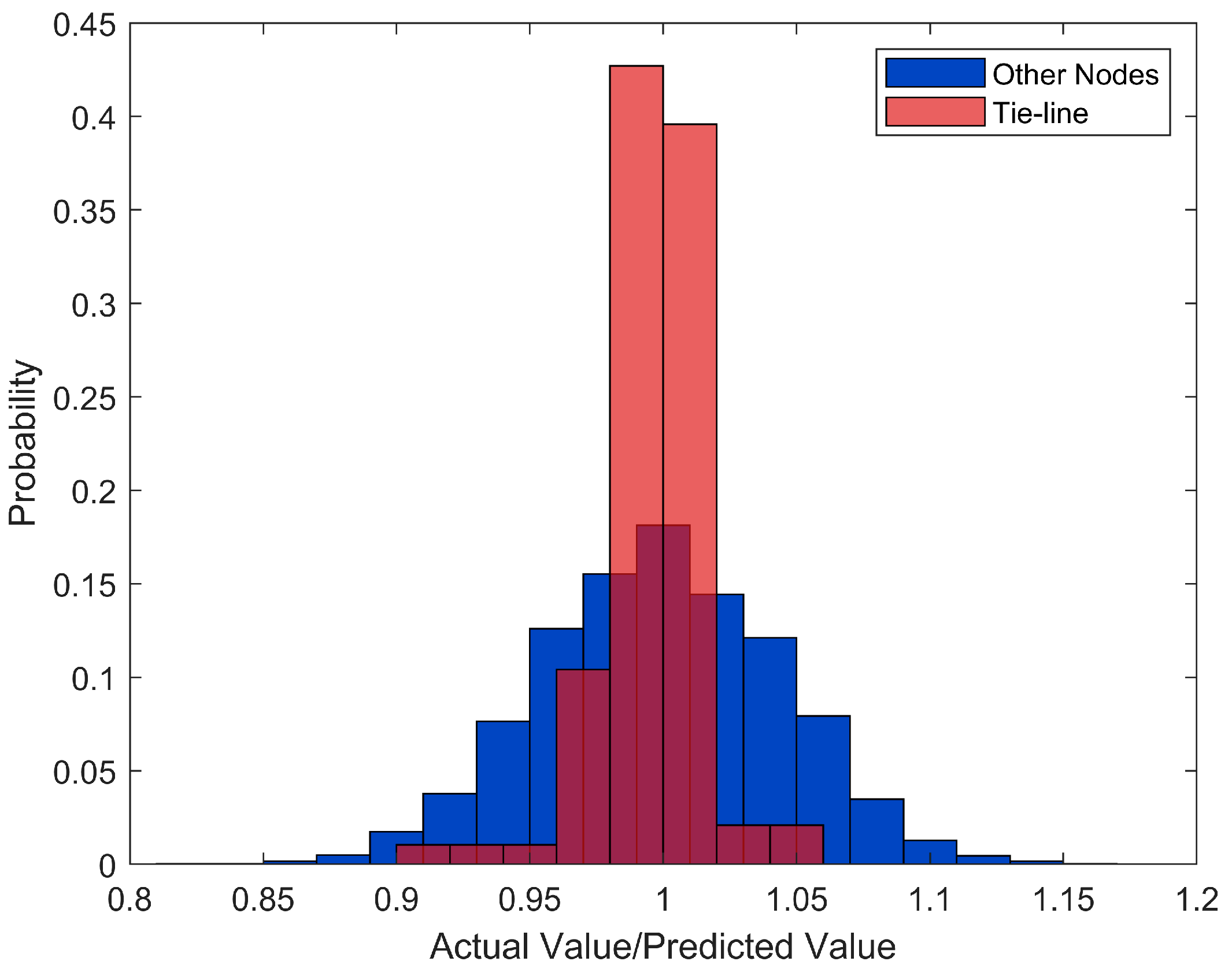
As mentioned above, the actual value deviates from the predicted value because the user’s behavior and the weather conditions cannot be predicted accurately. In the derivation of the SMPC model, the actual values of the PV and loads are considered to follow a normal distribution, and the mean is the predicted value with a variance of 0.002. The actual value will be obtained according to this probability distribution. The actual and predicted values are then divided to obtain a ratio, which is used as the x coordinate. The data for all moments of the day are counted to obtain statistics on the deviation between the actual and predicted values, as illustrated in Figure 5.

3.2. Performance Analysis

Firstly, the LPF model in this paper is compared with the traditional data-driven LPF model [44]. Data on the first 1000 s are used as the training set, with the assumption that only one initial round of training is performed in a day. We compared the voltage models for 32 nodes (except for node 0) to demonstrate the accuracy of this approach. Since the fluctuation of load and PV data from 0:00 to 6:00 is close to 0 (as shown in Figure 3), we use the data from 6:00 to 24:00 (64, 801 s, 32 nodes, and the total amount of data is 2, 073, 632).
The statistics for the relative error comparison are detailed in the Error section of Table 2. The relative error distribution is substantially better than that of the traditional model, and the ranges between the upper and lower quartiles and median are significantly lower. As the most typical indicators, the mean and median relative errors decreased by 95.13% and 97.36%, respectively. The above advantages are attributed to this model’s unique need for only a single initial training session for regression learning, with subsequent online updates based on real-time data measurements. Thus, this model lays a strong foundation for applying the LPF model to the SMPC model.
The Efficiency section in Table 2 presents a comparison of efficiency. Both methods are assumed to perform real-time updates. Here, the calculation environment is as follows: MATLAB R2018b, an i7-8750H 2.20 GHz Intel Core processor produced from Intel Corporation, 8 GB memory, and a Lenovo computer manufactured in Beijing, China. The LPF model used in this paper clearly has advantages in terms of the operation time and data burden. Although it takes a slightly longer time to initialize, this model can be used for a long period of time through online updates instead of retraining. The traditional model takes a shorter time to initialize, but the parameters cannot be updated online, which leads to frequent retraining in operation. Over the course of a 7-day run, the operation time and data burden decreased by 72.07% and 93.40%, respectively, under this method.
Next, we validate the proposed SMPC model. The scheduling interval is 15 min, and the prediction period T of SMPC is 10. It is assumed that the charging efficiency of ES is 0.95, and the discharging efficiency is 0.9. The power limit of ES is 0.15 MW , and the capacity is 0.4 MWh . We set the upper and lower limits of the node voltage to 1.00 and 0.95, respectively. The chance constraint requires that the voltage constraint be satisfied within a probability of 0.95, and the confidence level in sampling is set to 0.95. According to the corresponding formula, the number of samples N = 1340 is used. However, due to the uncertainty when using a large number of nodes, if the sampling is performed on each node at each time instant, the data burden is large. To solve this problem according to the characteristics of power flow, only the distant end nodes and nodes connected to PV and ES are selected to satisfy the voltage constraints with 0.95 probability. This selection is performed because the end node voltages are lower in the linear network, and nodes connected to PV may make the voltages higher. After the above simplification, the whole SMPC calculation process can be completed within 1 min, which greatly improves efficiency.
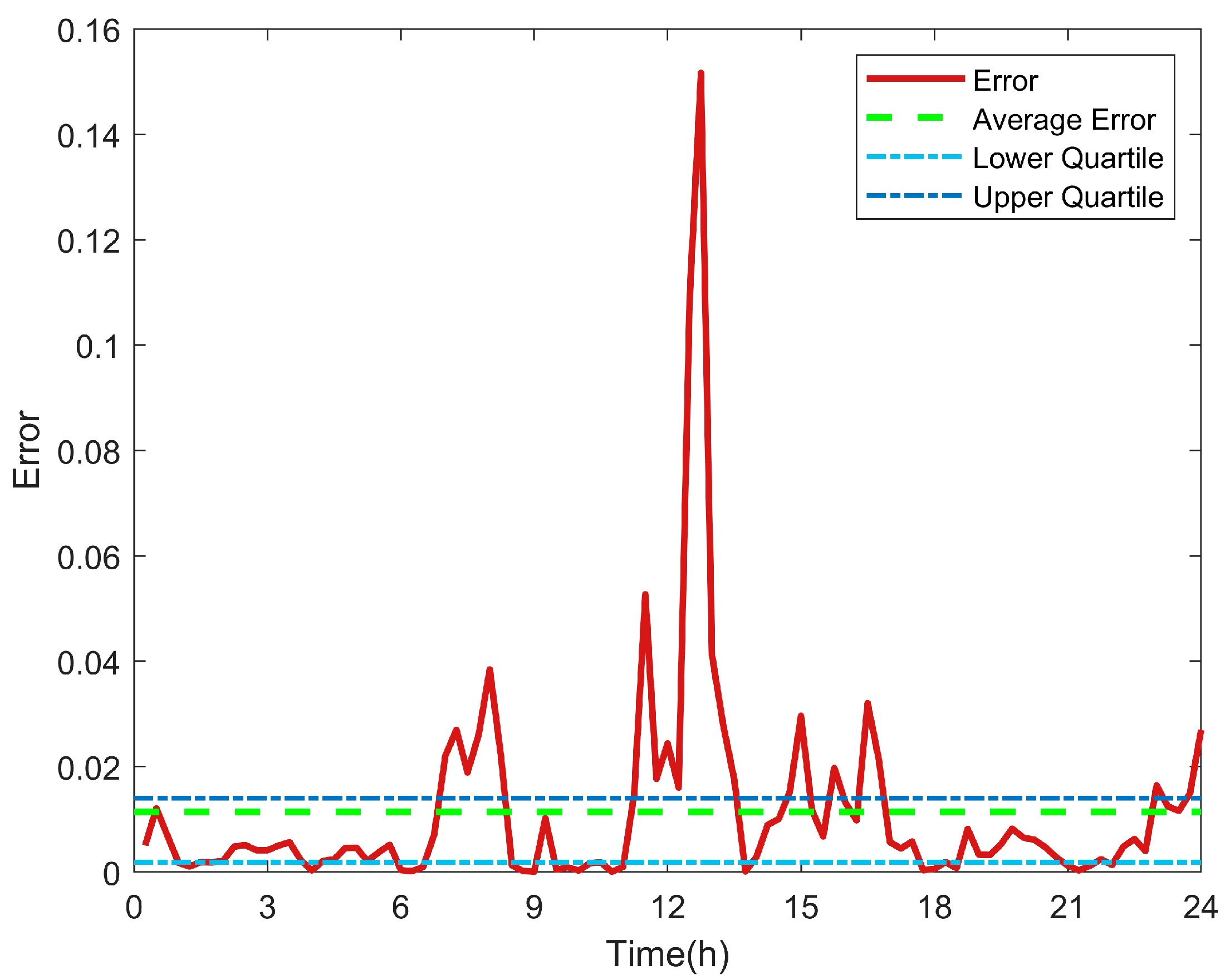
Figure 6 shows the power smoothing result, where the actual power of the tie-line closely follows the reference value. Figure 7 shows the relative error in Figure 6, where the mean relative error for the whole day is only 1.1%, and the upper and lower quartile are 1.4% and 0.2%, respectively. This result indicates that the proposed method can achieve excellent tie-line power smoothing by following the pre-set reference value.
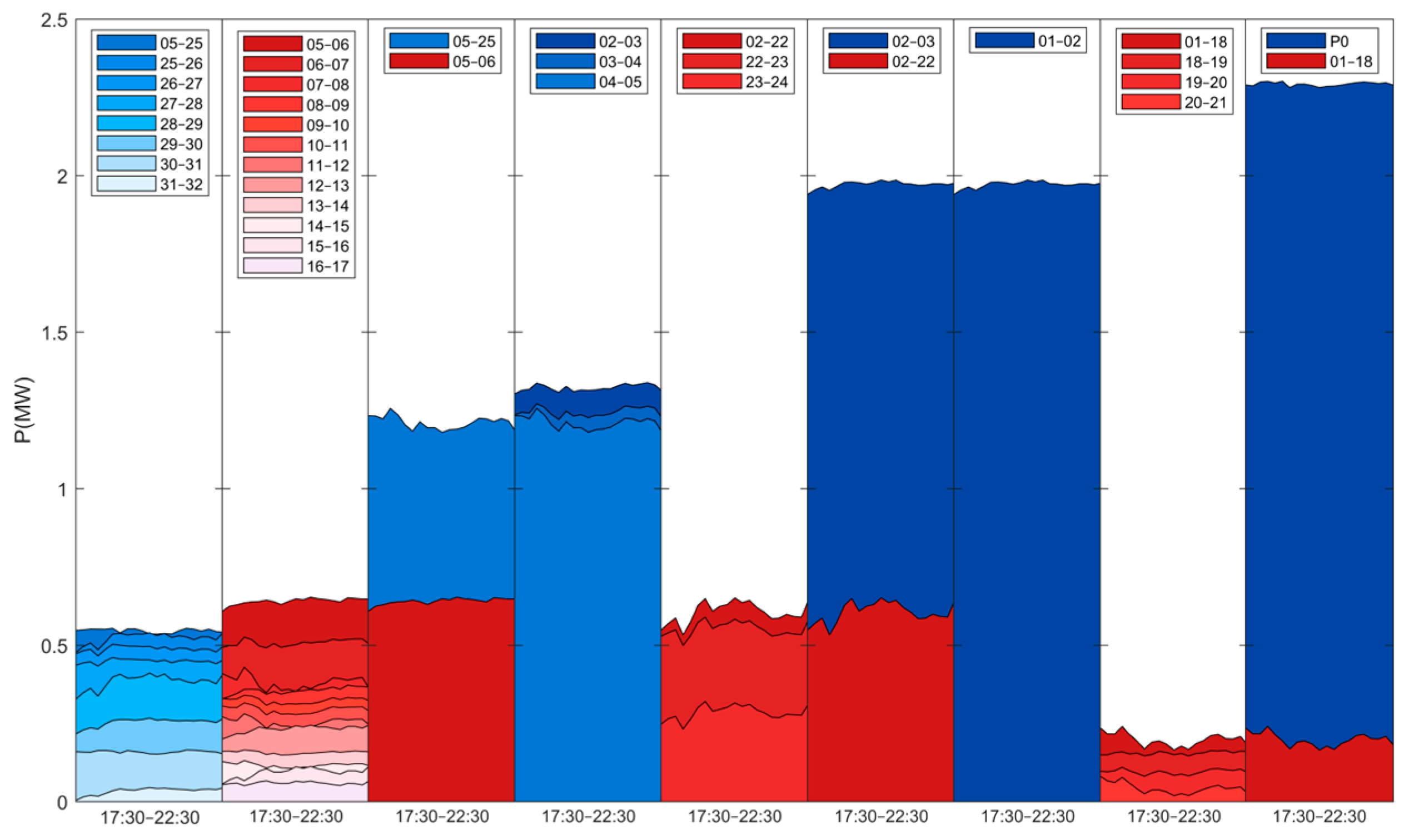
The reference value given in the analysis has many constant value periods. This result indicates that the power exchanged with the higher grid is not fluctuating. When this value is 0, the grid operates independently. Figure 8 illustrates the corresponding process. Here, the time period extends from 17:30 to 22:30, at which time the tie-line power reference value is constant. In both Figure 2 and Figure 8, the power network shown by the blue arrow is the selected backbone, with red lines representing the different branches injected into the backbone. The color from light to dark represents the increasing value of the power. The subplot from left to right represents the power demand of the trend from the end branch to node 0. With the cooperation of PV, ES, and load, the closer it comes to node 0, the smoother the power fluctuation becomes when performing calculations with the proposed SMPC model. Eventually, the power demand aggregated from all branches is constant at node 0. When analyzed in reverse, this result suggests that the constant power transmission from the higher grid during this period of time is controlled and distributed by the SMPC model to achieve a reasonable flow while ensuring voltage security. Further, when the tie-line power is controlled among multiple grids using the proposed method, the tie-line power of each grid can become a node with constant power or constant rate variation. In this way, larger grids can also be divided and controlled by the proposed method to realize control that cascades downward, such that multiple MGs can be interconnected and successfully operated independently. This process provides a distributed solution for scheduling and controlling multilevel or multiple MGs. The proposed method is also characterized by online updating, fast iterations, and efficient computations, which will provide powerful help for faster and more accurate scheduling needs.
Figure 9 presents a box chart of the voltage at each node throughout the day. No node exceeds the required range of 0.95 to 1.00, indicating that the proposed SMPC method controls the voltage well.
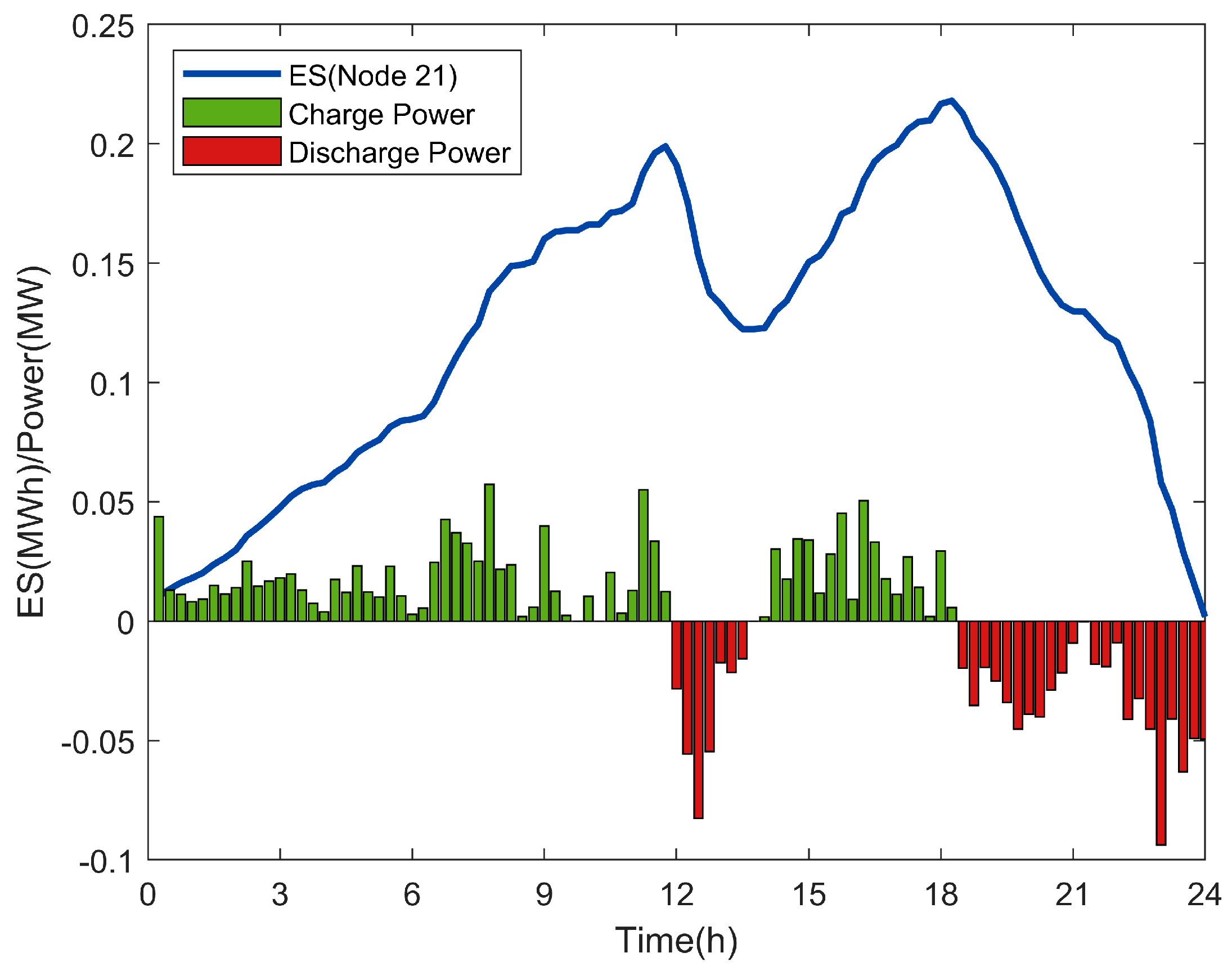
Figure 10 shows the charging and discharging of ES using node 21 as an example. Notably, the ES at node 21 was discharged during the midday period after 12:00 because the reference value at this time period was much lower than the predicted value when the reference value was set, as clearly illustrated in Figure 4. This factor caused a similar discharge pattern not only for the ES at node 21, but for all other ESs during this time period in order to meet requirements. The condition is stringent and extraordinary in order to verify that the proposed method still satisfies the tie-line smoothing requirements in extreme or special cases. The stability of the proposed method is theoretically demonstrated in Section 2.2, which indicates that this technique is effective in tie-line power smoothing and control. The excellent practical effects are more strongly demonstrated by the above performance analysis.
The proposed method achieves tie-line power smoothing by following a pre-set reference value and accommodates uncertainty locally at the user side through strong cooperation by flexibly adjusting the ES and PV elements. This study also indicates that the proposed method can better handle uncertainty and offer more accurate results. Overall, the proposed technique is a forward-looking, stable, fast, and efficient calculation method.

4. Conclusions

In this paper, a data-driven SMPC method for tie-line power smoothing under uncertainty is proposed. This type of method is a major priority due to the high proportion of DER access in the distributed network. To satisfy the state equation format that represents the cornerstone of the SMPC model, this method applies a novel data-driven LPF model. We developed this model by performing Taylor expansion on a trained quadratic model after regression learning. After initial training, the model can be updated online without retraining, which significantly reduces the data burden and operational costs. Compared to the traditional data-driven LPF model, the mean and median relative errors of the proposed model in actual cases decreased by 95.13% and 97.36%, respectively, and the operation time and data burden decreased by 72.07% and 93.40% over the 7 days of operation.
For handling uncertainty, the tie-line power smoothing model is derived by combining stochastic optimization with the standard MPC method to form the SMPC model. Finally, the SMPC model is simplified using the scenario method. Compared to existing models, the proposed method achieves tie-line power smoothing through collaboration between DERs using SMPC and considers the time-coupling characteristics of DER to enable long-term scale optimization. Ultimately, this model is prospective, stable, and resistant to perturbations, with small errors and low operating costs. The performance analysis further indicated that the SMPC model can effectively and accurately realize tie-line power control and smoothing. The mean relative error is only 1.1%, with upper and lower quartiles of 1.4% and 0.2%, respectively, demonstrating the superiority of the proposed method.

Author Contributions

Methodology, M.A.; software, M.A.; writing—original draft preparation, M.A.; writing—review and editing, X.H. and T.L. All authors have read and agreed to the published version of the manuscript.

Funding

This research was funded by Shandong Excellent Youth Science Fund Program (Overseas), grant number 2022HWYQ-039.

Data Availability Statement

The original contributions presented in the study are included in the article. Further enquiries can be directed to the corresponding author.

Conflicts of Interest

The authors declare no conflicts of interest.

References

  1. Li, Z.M.; Xu, Y.; Wang, P.; Xiao, G.X. Restoration of a Multi-Energy Distribution System With Joint District Network Reconfiguration via Distributed Stochastic Programming. IEEE Trans. Smart Grid 2024, 15, 2667–2680. [Google Scholar] [CrossRef]
  2. Dall’Anese, E.; Dhople, S.V.; Giannakis, G.B. Photovoltaic Inverter Controllers Seeking AC Optimal Power Flow Solutions. IEEE Trans. Power Syst. 2016, 31, 2809–2823. [Google Scholar] [CrossRef]
  3. Liu, Y.; Li, Y.Z.; Xin, H.H.; Gooi, H.B.; Pan, J.F. Distributed Optimal Tie-Line Power Flow Control for Multiple Interconnected AC Microgrids. IEEE Trans. Power Syst. 2019, 34, 1869–1880. [Google Scholar] [CrossRef]
  4. Zhang, C.; Lin, W.; Ke, D.P.; Sun, Y.Z. Smoothing Tie-Line Power Fluctuations for Industrial Microgrids by Demand Side Control: An Output Regulation Approach. IEEE Trans. Power Syst. 2019, 34, 3716–3728. [Google Scholar] [CrossRef]
  5. Zhang, R.; Yu, J.L. External tie line power fluctuations smoothing strategy of new urban power grid. Int. J. Electr. Power Energy Syst. 2023, 153, 109289. [Google Scholar] [CrossRef]
  6. Said, S.M.; Ali, A.; Hartmann, B. Tie-line Power Flow Control Method for Grid-connected Microgrids with SMES Based on Optimization and Fuzzy Logic. J. Mod. Power Syst. Clean Energy 2020, 8, 941–950. [Google Scholar] [CrossRef]
  7. Xiao, Z.X.; Guerrero, J.M.; Shuang, J.; Sera, D.; Schaltz, E.; Vásquez, J.C. Flat tie-line power scheduling control of grid-connected hybrid microgrids. Appl. Energy 2018, 210, 786–799. [Google Scholar] [CrossRef]
  8. Che, Y.B.; Zhou, J.H.; Lin, T.J.; Li, W.X.; Xu, J.M. A Simplified Control Method for Tie-Line Power of DC Micro-Grid. Energies 2018, 11, 933. [Google Scholar] [CrossRef]
  9. Ding, Y.; Xie, D.J.; Hui, H.X.; Xu, Y.; Siano, P. Game-Theoretic Demand Side Management of Thermostatically Controlled Loads for Smoothing Tie-Line Power of Microgrids. IEEE Trans. Power Syst. 2021, 36, 4089–4101. [Google Scholar] [CrossRef]
  10. Mudaliyar, S.; Duggal, B.; Mishra, S. Distributed Tie-Line Power Flow Control of Autonomous DC Microgrid Clusters. IEEE Trans. Power Electron. 2020, 35, 11250–11266. [Google Scholar] [CrossRef]
  11. Wang, D.; Zhi, Y.Q.; Yu, B.; Chen, Z.Y.; An, Q.S.; Cheng, L.; Fan, M.H. Optimal Coordination Control Strategy of Hybrid Energy Storage Systems for Tie-line Smoothing Services in Integrated Community Energy Systems. CSEE J. Power Energy 2018, 4, 408–416. [Google Scholar] [CrossRef]
  12. Khavari, F.; Badri, A.; Zangeneh, A. A tie-line power smoothing via a novel dynamic real-time pricing mechanism in MMGs. Int. J. Electr. Power Energy Syst. 2022, 136, 107671. [Google Scholar] [CrossRef]
  13. Islam, M.; Yang, F.W.; Amin, M. Dynamic control of grid-connected microgrids for tie-line smoothing. Int. Trans. Electr. Energy Syst. 2020, 30, 12557. [Google Scholar] [CrossRef]
  14. Xu, J.; Liao, S.Y.; Jiang, H.Y.; Zhang, D.N.; Sun, Y.Z.; Ke, D.P.; Li, X.; Yang, J.; Peng, X.T.; Yao, L.Z. A Multi-time Scale Tie-line Energy and Reserve Allocation Model Considering Wind Power Uncertainties for Multi-area Systems. CSEE J. Power Energy 2021, 7, 677–687. [Google Scholar] [CrossRef]
  15. Li, Z.M.; Xu, Y.; Wang, P.; Xiao, G.X. Coordinated preparation and recovery of a post-disaster Multi-energy distribution system considering thermal inertia and diverse uncertainties. Appl. Energy 2023, 336, 120736. [Google Scholar] [CrossRef]
  16. Fan, S.; He, G.Y.; Zhou, X.Y.; Cui, M.J. Online Optimization for Networked Distributed Energy Resources With Time-Coupling Constraints. IEEE Trans. Smart Grid 2021, 12, 251–267. [Google Scholar] [CrossRef]
  17. Chen, S.; Wang, C.F.; Zhang, Z.W. Multitime Scale Active and Reactive Power Coordinated Optimal Dispatch in Active Distribution Network Considering Multiple Correlation of Renewable Energy Sources. IEEE Trans. Ind. Appl. 2021, 57, 5614–5625. [Google Scholar] [CrossRef]
  18. Guo, Y.F.; Wu, Q.W.; Gao, H.L.; Huang, S.; Zhou, B.; Li, C.B. Double-Time-Scale Coordinated Voltage Control in Active Distribution Networks Based on MPC. IEEE Trans. Sustain. Energy 2020, 11, 294–303. [Google Scholar] [CrossRef]
  19. Zheng, Y.; Li, S.Y.; Tan, R.M. Distributed Model Predictive Control for On-Connected Microgrid Power Management. IEEE Trans. Control. Syst. Technol. 2018, 26, 1028–1039. [Google Scholar] [CrossRef]
  20. Cai, S.; Xie, Y.Y.; Wu, Q.W.; Zhang, M.L.; Jin, X.L.; Xiang, Z.R. Active and Reactive Power Coordinated Two-Stage MG Scheduling for Resilient Distribution Systems Under Uncertainties. IEEE Trans. Smart Grid 2022, 13, 2986–2998. [Google Scholar] [CrossRef]
  21. Ding, Y.F.; Morstyn, T.; McCulloch, M.D. Distributionally Robust Joint Chance-Constrained Optimization for Networked Microgrids Considering Contingencies and Renewable Uncertainty. IEEE Trans. Smart Grid 2022, 13, 2467–2478. [Google Scholar] [CrossRef]
  22. Mesbah, A. Stochastic Model Predictive Control: An Overview and Perspectives for Future Research. IEEE Control. Syst. Mag. 2016, 36, 30–44. [Google Scholar] [CrossRef]
  23. Zhao, Z.L.; Guo, J.T.; Luo, X.; Lai, C.S.; Yang, P.; Lai, L.L.; Li, P.; Guerrero, J.M.; Shahidehpour, M. Distributed Robust Model Predictive Control-Based Energy Management Strategy for Islanded Multi-Microgrids Considering Uncertainty. IEEE Trans. Smart Grid 2022, 13, 2107–2120. [Google Scholar] [CrossRef]
  24. Zhang, Z.W.; Wang, C.F.; Wu, Q.W.; Dong, X.M. Optimal dispatch for cross-regional integrated energy system with renewable energy uncertainties: A unified spatial-temporal cooperative framework. Energy 2024, 292, 130433. [Google Scholar] [CrossRef]
  25. Jabr, R.A. Linear Decision Rules for Control of Reactive Power by Distributed Photovoltaic Generators. IEEE Trans. Power Syst. 2018, 33, 2165–2174. [Google Scholar] [CrossRef]
  26. Yang, Z.F.; Zhong, H.W.; Bose, A.; Zheng, T.X.; Xia, Q.; Kang, C.Q. A Linearized OPF Model with Reactive Power and Voltage Magnitude: A Pathway to Improve the MW-Only DC OPF. IEEE Trans. Power Syst. 2018, 33, 1734–1745. [Google Scholar] [CrossRef]
  27. Wang, B.B.; Tang, N.; Bo, R.; Li, F.X. Three-phase DLMP model based on linearized power flow for distribution with application to DER benefit studies. Int. J. Electr. Power Energy Syst. 2021, 130, 106884. [Google Scholar] [CrossRef]
  28. Sperr, F.; Stai, E.; Venkatraman, A.; Krause, T.; Hug, G. Service Restoration in the Medium Voltage Grid Minimizing the SAIDI Contribution After Primary Substation Failures. IEEE Trans. Power Syst. 2024, 39, 66–82. [Google Scholar] [CrossRef]
  29. Tan, Y.; Chen, Y.Y.; Li, Y.; Cao, Y.J. Linearizing Power Flow Model: A Hybrid Physical Model-Driven and Data-Driven Approach. IEEE Trans. Power Syst. 2020, 35, 2475–2478. [Google Scholar] [CrossRef]
  30. Li, Z.G.; Yu, J.Y.; Wu, Q.H. Approximate Linear Power Flow Using Logarithmic Transform of Voltage Magnitudes with Reactive Power and Transmission Loss Consideration. IEEE Trans. Power Syst. 2018, 33, 4593–4603. [Google Scholar] [CrossRef]
  31. Liu, Y.T.; Li, Z.S.; Zhou, Y. Data-Driven-Aided Linear Three-Phase Power Flow Model for Distribution Power Systems. IEEE Trans. Power Syst. 2022, 37, 2783–2795. [Google Scholar] [CrossRef]
  32. Shao, Z.T.; Zhai, Q.Z.; Wu, J.; Guan, X.H. Data Based Linear Power Flow Model: Investigation of a Least-Squares Based Approximation. IEEE Trans. Power Syst. 2021, 36, 4246–4258. [Google Scholar] [CrossRef]
  33. Liu, Y.T.; Li, Z.S.; Zhao, J.B. Robust Data-Driven Linear Power Flow Model with Probability Constrained Worst-Case Errors. IEEE Trans. Power Syst. 2022, 37, 4113–4116. [Google Scholar] [CrossRef]
  34. Liu, Y.X.; Wang, Y.; Zhang, N.; Lu, D.; Kang, C.Q. A Data-Driven Approach to Linearize Power Flow Equations Considering Measurement Noise. IEEE Trans. Smart Grid 2020, 11, 2576–2587. [Google Scholar] [CrossRef]
  35. Liu, Y.X.; Zhang, N.; Wang, Y.; Yang, J.W.; Kang, C.Q. Data-Driven Power Flow Linearization: A Regression Approach. IEEE Trans. Smart Grid 2019, 10, 2569–2580. [Google Scholar] [CrossRef]
  36. An, M.L.; Lu, T.G.; Han, X.S. An online updated linear power flow model based on regression learning. IET Gener. Transm. Distrib. 2024, 18, 2006–2019. [Google Scholar] [CrossRef]
  37. Li, Z.M.; Wu, L.; Xu, Y.; Wang, L.H.; Yang, N. Distributed tri-layer risk-averse stochastic game approach for energy trading among multi-energy microgrids. Appl. Energy 2023, 331, 120282. [Google Scholar] [CrossRef]
  38. Bertsekas, D.P.; Tsitsiklis, J.N.; Tsitsiklis, J.N. Introduction to Probability, 2nd ed.; Athena Scientific: Belmont, MA, USA, 2008. [Google Scholar]
  39. Alamo, T.; Tempo, R.; Luque, A. On the Sample Complexity of Randomized Approaches to the Analysis and Design under Uncertainty. In Proceedings of the 2010 American Control Conference, Baltimore, MD, USA, 30 June–2 July 2010; pp. 4671–4676. [Google Scholar]
  40. Campi, M.C.; Garatti, S. A Sampling-and-Discarding Approach to Chance-Constrained Optimization: Feasibility and Optimality. J. Optim. Theory Appl. 2011, 148, 257–280. [Google Scholar] [CrossRef]
  41. Cannon, M.; Kouvaritakis, B.; Wu, X. Model predictive control for systems with stochastic multiplicative uncertainty and probabilistic constraints. Automatica 2009, 45, 167–172. [Google Scholar] [CrossRef]
  42. Cannon, M.; Kouvaritakis, B.; Wu, X.J. Probabilistic Constrained MPC for Multiplicative and Additive Stochastic Uncertainty. IEEE Trans. Autom. Control 2009, 54, 1626–1632. [Google Scholar] [CrossRef]
  43. Campi, M.C.; Garatti, S.; Prandini, M. The scenario approach for systems and control design. Annu. Rev. Control 2009, 33, 149–157. [Google Scholar] [CrossRef]
  44. Chen, Y.B.; Wu, C.; Qi, J.J. Data-driven Power Flow Method Based on Exact Linear Regression Equations. J. Mod. Power Syst. Clean Energy 2022, 10, 800–804. [Google Scholar] [CrossRef]
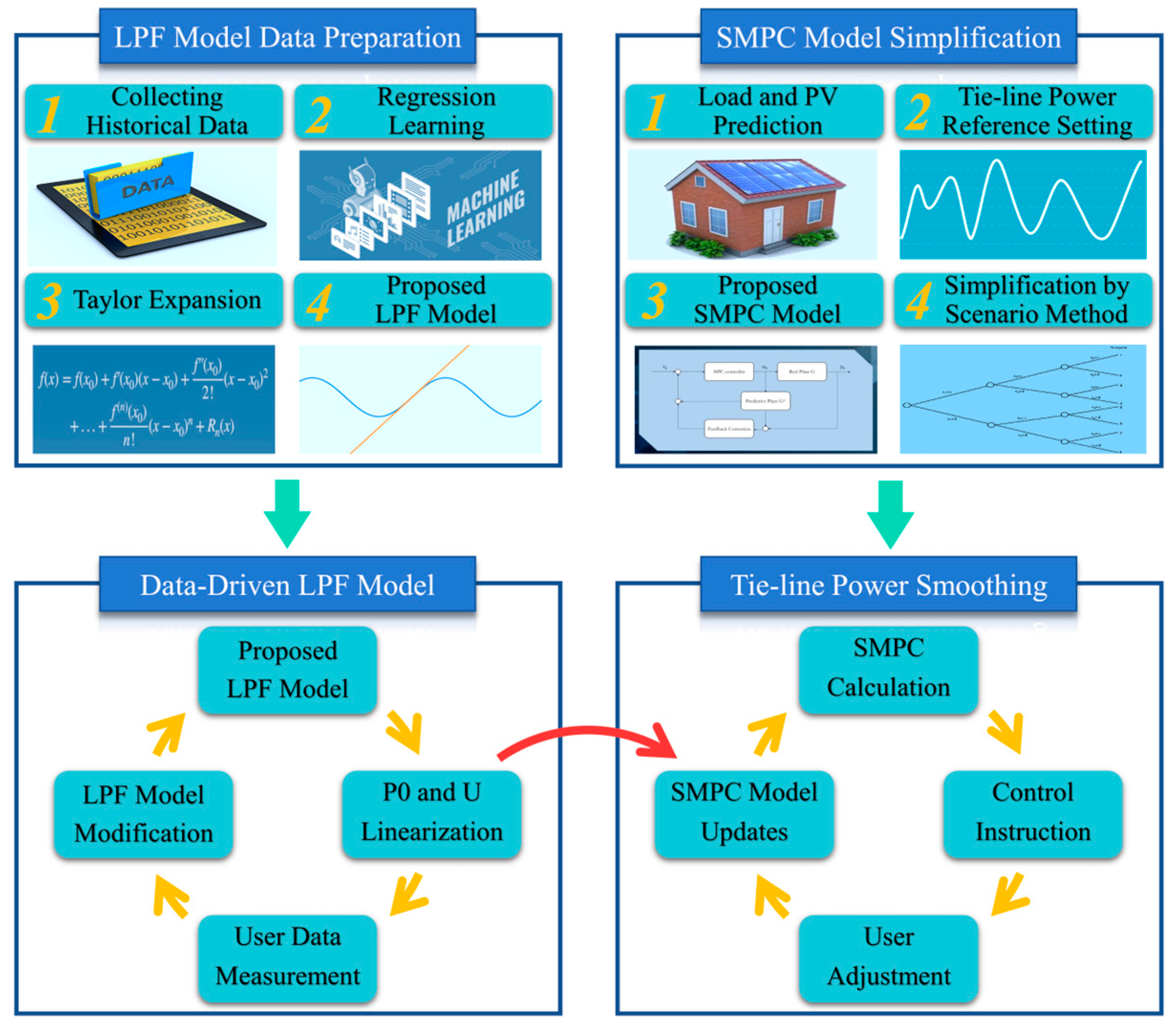
Figure 1. Flowchart of the proposed method.
Energies 17 03515 g001
Figure 2. Power network structure.
Energies 17 03515 g002
Figure 3. Typical loads and PV over a day.
Energies 17 03515 g003
Figure 4. Setting of the reference values of tie-line power.
Energies 17 03515 g004
Figure 5. Analysis of the actual and predicted values.
Energies 17 03515 g005
Figure 6. Tie-line power smoothing result.
Energies 17 03515 g006
Figure 7. Error of the tie-line power smoothing result.
Energies 17 03515 g007
Figure 8. Decomposition of the power flow after the proposed SMPC method.
Energies 17 03515 g008
Figure 9. Range of node voltages over a day.
Energies 17 03515 g009
Figure 10. Operation of ES.
Energies 17 03515 g010
Table 1. Comparison between the proposed method and the existing literature.
LiteratureMethodologyVoltage ControlESUncertaintyTime ScalePower Flow Control Method
[3]Distributed optimal tie-line power flow control for the multiple-MG system.Not consideredNot consideredNot consideredLongNonlinearOptimization
[4]Output regulation approach combined with LQ optimal controlConsideredNot consideredNot consideredShortLinearModern Control
[5] External tie line power fluctuations smoothing strategy of new urban power grid Not consideredConsideredConsideredLongNonlinearOptimization
[6] Fuzzy logic control based and optimized fuzzy logic control based SMES methodConsideredConsideredNot consideredShortNonlinearOptimization
[7] Flat tie-line power scheduling control of grid-connected hybrid MGsConsideredConsideredNot consideredShortNonlinearClassical Control
[8]Improved droop control strategy for tie-line power of DC-MG ConsideredConsideredNot consideredShortNonlinearClassical Control
[9]Game-theoretic demand side management for smoothing tie-line power Not consideredNot consideredConsideredLongNonlinearGame Theory
[10]A unifying hierarchical control scheme based on distributed communicationConsideredConsideredNot consideredShortNonlinearClassical Control
[11]Optimal coordination control for tie-line smoothing in hybrid energy storage systems Not consideredConsideredNot consideredLongNonlinearModern Control
[12]A tie-line power smoothing via a novel dynamic real-time pricing mechanism in multi-MGNot consideredConsideredConsideredShortLinearOptimization
[13]Dynamic control of grid-connected MGs for tie-line smoothingConsideredConsideredNot consideredShortNonlinearModern Control
[14]A multi-time-scale tie-line energy and reserve allocation model Not consideredNot consideredConsideredLongLinearOptimization
This paperSMPC for the tie-line power smoothing with a novel data-driven LPF modelConsideredConsideredConsideredLongLinearSMPC
Table 2. Comparison result of error and efficiency.
SectionIndexThe Traditional Data-Driven LPFThe Proposed MethodImprovement
ErrorMaximum of relative error1.73960%0.32083%81.56%
Upper quartile of relative error0.43340%0.01578%96.36%
Mean of relative error0.27041%0.01317%95.13%
Median of relative error0.15968%0.00421%97.36%
Lower quartile of relative error0.04535%0.00070%98.47%
Minimum of relative error0.00019%0%100%
EfficiencyTime for initializing0.016 s24.88 s/
Data burden for initializing1455 KB678 KB53.40%
Time for model updating once0.016 s0.002 s87.50%
Data burden for model updating once1455 KB96 KB93.40%
Time for total operation (per minute in 7 days)161.28 s45.04 s72.07%
Data burden for total operation (per minute in 7 days)13.987 GB0.923 GB93.40%
Disclaimer/Publisher’s Note: The statements, opinions and data contained in all publications are solely those of the individual author(s) and contributor(s) and not of MDPI and/or the editor(s). MDPI and/or the editor(s) disclaim responsibility for any injury to people or property resulting from any ideas, methods, instructions or products referred to in the content.