
Multi-Site Wind Speed Prediction Based on Graph Embedding and Cyclic Graph Isomorphism Network (GIN-GRU)


Abstract
1. Introduction
2. Materials and Methods
2.1. Construction of Graph Networks
2.1.1. PCA-RF Fusion Model
2.1.2. Random Forests
2.1.3. Principal Component Analysis
2.1.4. PCA-RF Feature Fusion
- (1)
- Build a random forest. Bootstrap sampling and random feature selection techniques are utilized to generate a training dataset and a corresponding subset of features. These elements form the basis for constructing an individual decision tree. The process of building a decision tree involves randomly selecting a subset of the dataset and recursively splitting the nodes based on optimal segmentation criteria until the stopping criteria of the random forest are met. Through the repetition of this process, a random forest model is assembled with I different decision trees, where the i-th decision tree has T nodes and C categories.
- (2)
- Calculate the Gini impurity and the amount of its variation. In tree i, at node j, it is essential to calculate the proportion of category c, represented as , against the total categories. The variation in Gini impurity is then determined by evaluating the Gini impurity before and after the branching of node j. The calculation formula is as follows:where j = 1, 2…T, i = 1, 2…I, k = 1, 2…M, c = 1, 2…C. and represent the two new nodes after node j is branched. are feature vector reduction of Gini impurity after node splitting in decision tree i.
- (3)
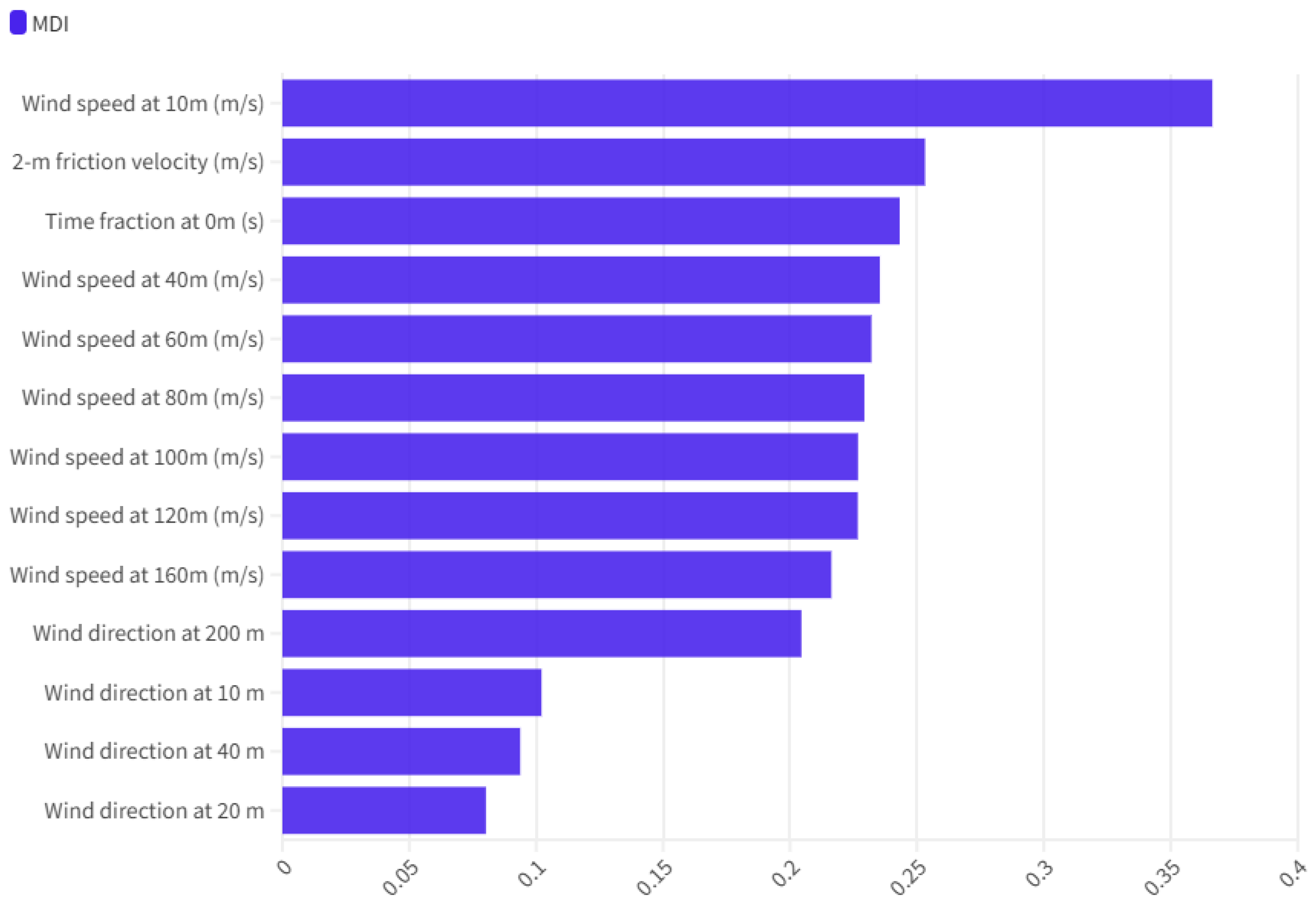
- Calculate the MDI. MDI for feature is as follows:
- (4)
- Feature selection. In the feature selection phase, features are ranked by their MDI values. Subsequently, a threshold denoted by γ is determined. Features with an MDI value of are selected to comprise the primary feature matrix , which includes features. Conversely, features with an MDI value of are used to construct the auxiliary matrix , which incorporates the remaining features.
- (5)
- Feature decentralization. The auxiliary matrix is decentralized to yield the matrix .where is the auxiliary matrix .
- (6)
- Compute eigenvalues and eigenvectors. The eigenvalue decomposition is performed on the covariance matrix. The feature values are ranked in descending order and sequentially aggregated until the cumulative contribution rate, denoted by . Consequently, in adherence to this criterion, the primary r features are chosen to constitute the matrix of .where is a set of eigenvalues, is the matrix of eigenvectors.
- (7)
- Data dimensionality reduction. We calculate the dimensionality reduction matrix utilizing the subsequent formula:
- (8)
- Matrix splicing. By horizontally concatenating the matrices and , we obtain a matrix of dimension .
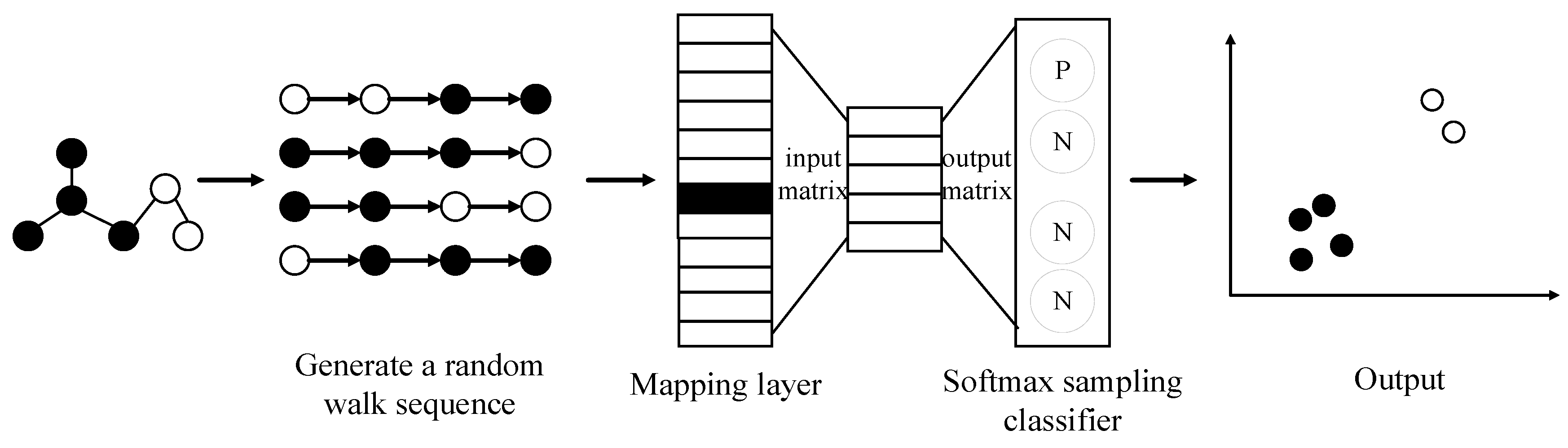
2.1.5. Integrative Modeling of Graph Embeddings and Mahalanobis Distances
2.1.6. Construction of Predefined Graphs
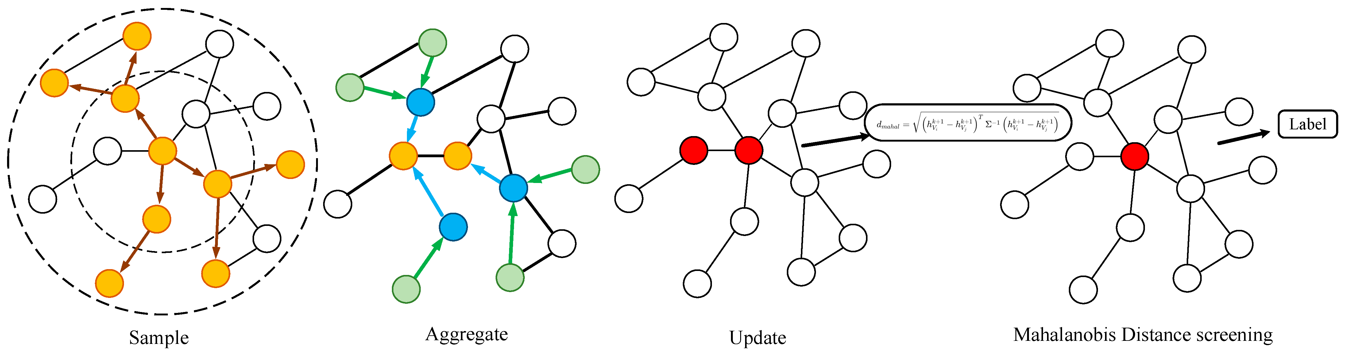
2.1.7. GraphSAGE-Based Graph Embedding
- A.
- Sampling: for node , we randomly sample a subset of its neighboring nodes from the set of its neighbor nodes to create a subgraph. This method decreases computational demands yet preserves the heterogeneity among adjacent nodes.
- B.
- Aggregation: for node , we employ an aggregation function that compresses and transforms the feature vectors of its neighboring nodes to generate a new feature vector through aggregation. The formula for aggregation is expressed aswhere denotes the node in the first k layer of the embedding vector, and is the feature vector of node . denotes the sigmoid activation function. The matrix represents the learnable weights. signifies the splicing operation. is the aggregation function at the first k layer and refers to the node neighboring set.
- C.
- Update: for node , the feature vector is concatenated with the aggregated feature vector . This combined vector then passes through a fully connected layer followed by an activation function, which results in the embedding vector for node . This process facilitates the integration and nonlinear transformation of the features represented by node with those of its neighboring nodes. The updated formula is expressed as follows:where denotes the splicing or summing operation and denotes the learnable weight matrix.
2.1.8. Modification of Graph Network Edges
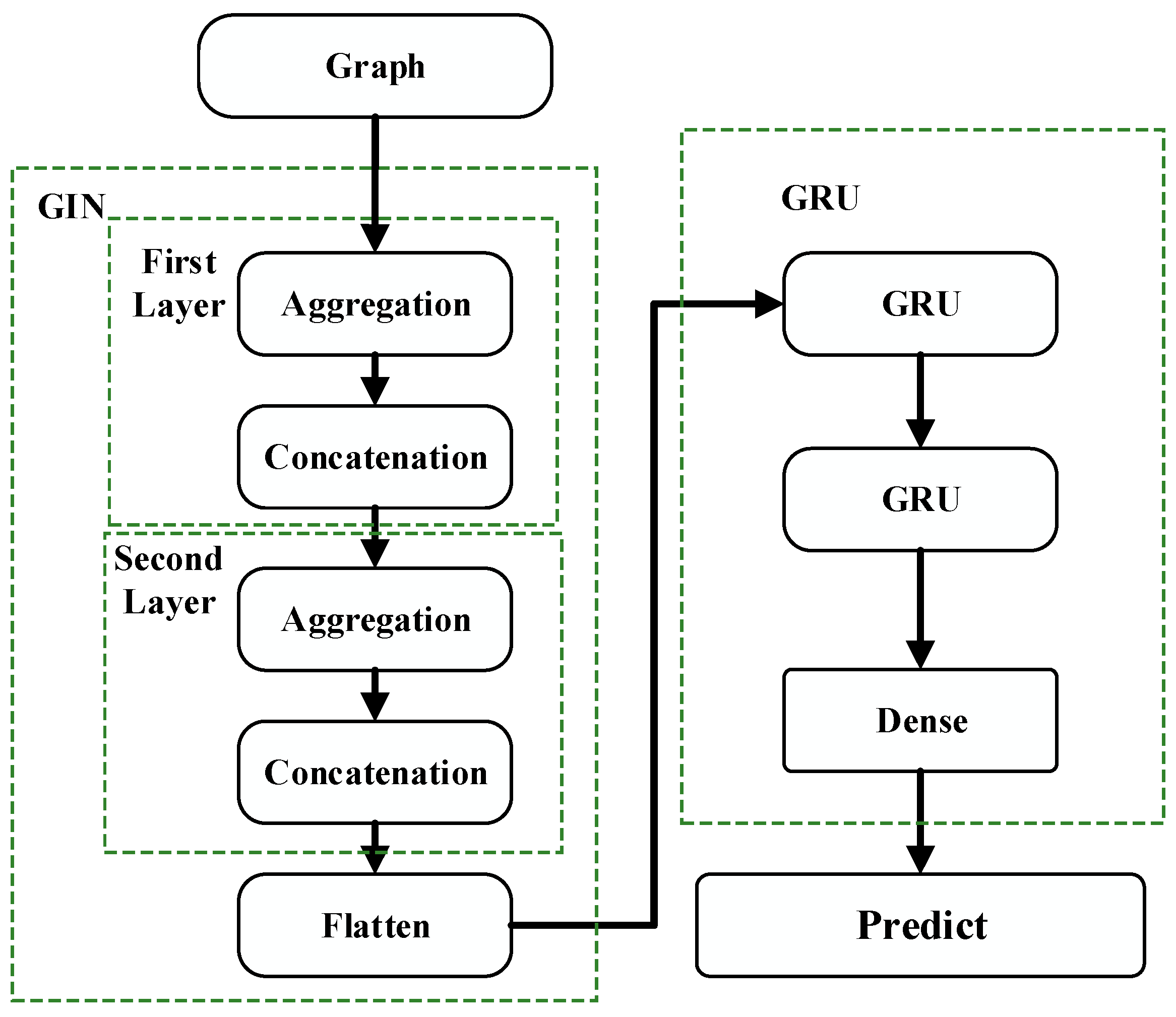
2.2. Spatio-Temporally Integrated Forecasting Model Based on GIN and GRU
2.2.1. Graph Isomorphism Network
- (1)
- Aggregation. The GIN model employs a summation aggregation function to compile the feature vectors from the neighboring nodes of node , which aims to integrate the information from all adjacent nodes.where is the temporary aggregation result at layer k, which contains only the information of neighboring nodes.
- (2)
- Combination. The aggregated features of neighboring nodes are combined with the target node and the features from the previous layer to form a new node feature . This process, facilitated by learnable parameters and the nonlinear transformations of a multilayer perceptron (MLP), enhances the model’s ability to learn and represent complex patterns.where is a trainable parameter that allows the model to adjust the self-loop when updating the node features with the contribution. is the final node feature representation after combination.
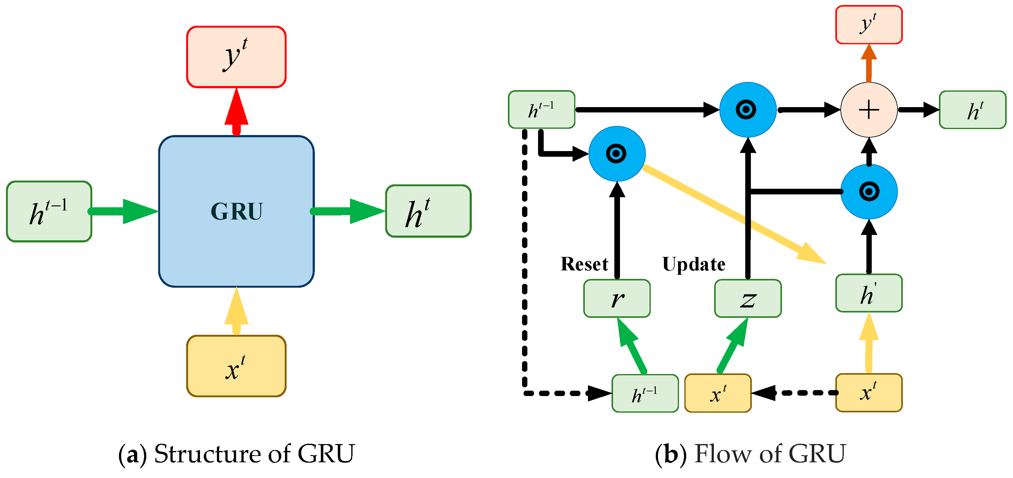
2.2.2. Gated Recurrent Unit
- (1)
- Determine the values of the update and reset gates. The update gate assesses the degree to which the hidden state from the preceding timestep is retained in the current timestep. Conversely, the reset gate regulates the proportion of the previous timestep’s hidden state that is incorporated into the computation of the current state. The formula for this step is given bywhere and denote the values of the update gate and the reset gate, respectively. The sigmoid activation function, represented by , is utilized to facilitate the computation of gradients and enable effective backpropagation. The weight matrices and , along with the bias vectors and , play a pivotal role in this mechanism. Additionally, represents the hidden state from the previous timestep, while corresponds to the input at the current timestep.
- (2)
- Compute the candidate hidden state. This represents the candidate hidden state, obtained by applying the hyperbolic tangent () activation function to the current input and the previously reset hidden state. The formulas are expressed as follows:where is the candidate hidden state, is the weight matrix, is the bias vector, and represents the element-wise multiplication operation.
- (3)
- Compute the current hidden state. The current hidden state is computed as the weighted average of the previous hidden state and the candidate hidden state, where the weights are governed by the update gate. The formulas are expressed as follows:where represents the hidden state at the current moment, denotes the value of the update gate, and is the candidate hidden state.
2.3. Hybrid Model of GE-GIN-GRU Network
3. Results
3.1. Datasets and Settings
3.1.1. Dataset
3.1.2. Experimental Equipment
3.1.3. Error Assessment Criteria
3.2. Experimental Results and Analysis
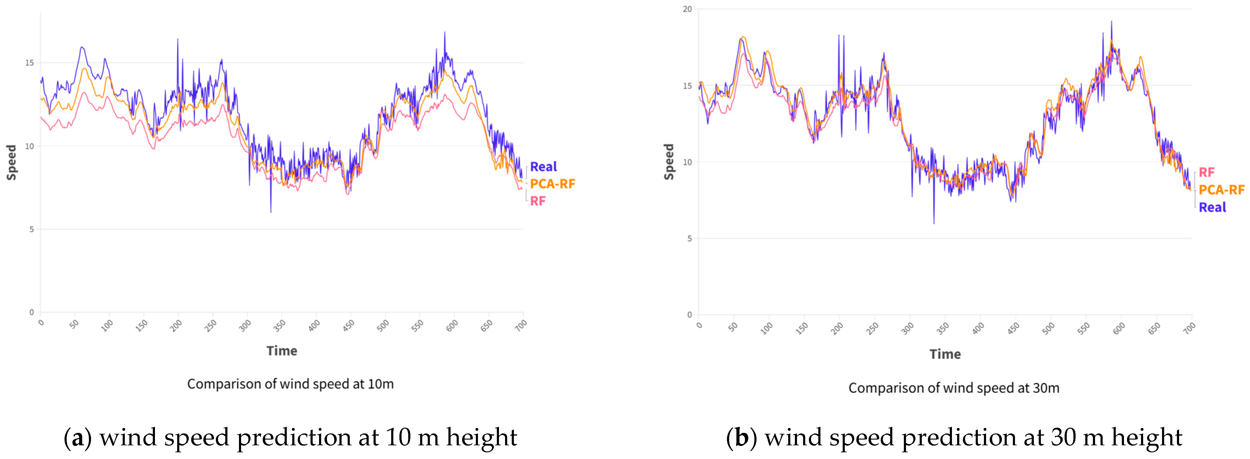
3.2.1. Analysis of PCA-RF
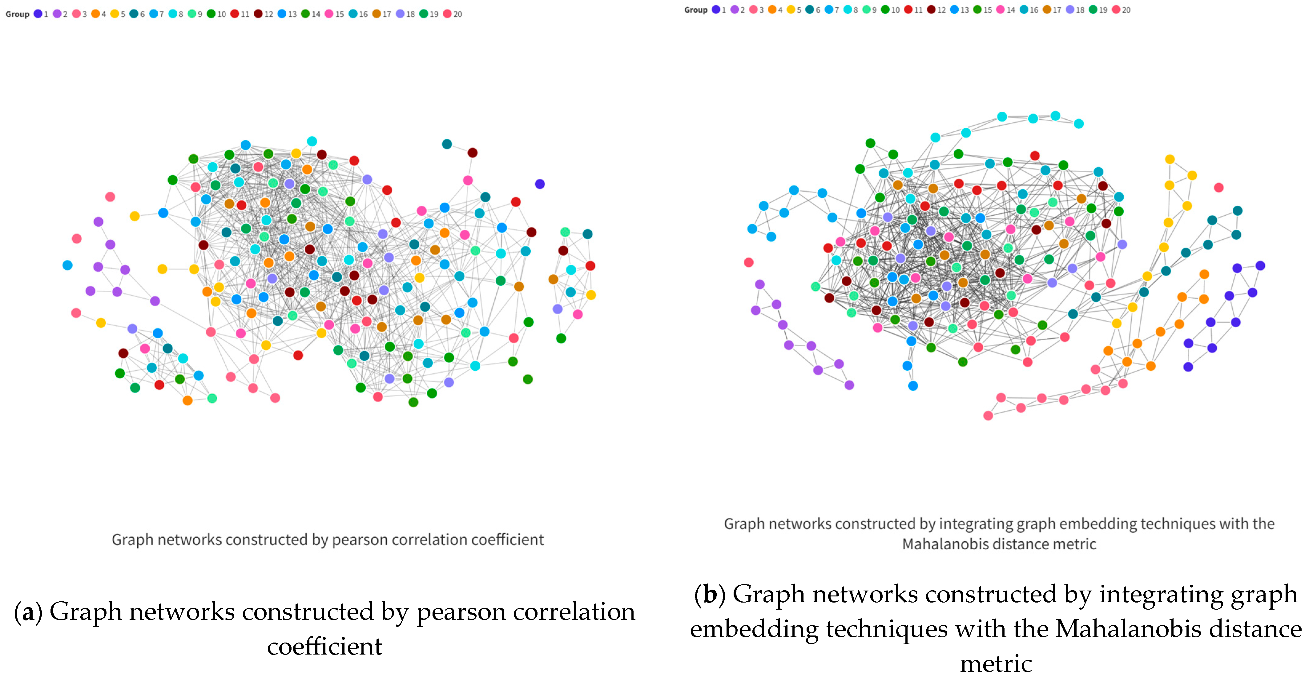
3.2.2. Evaluation of Graph Embedding for Graph Networks
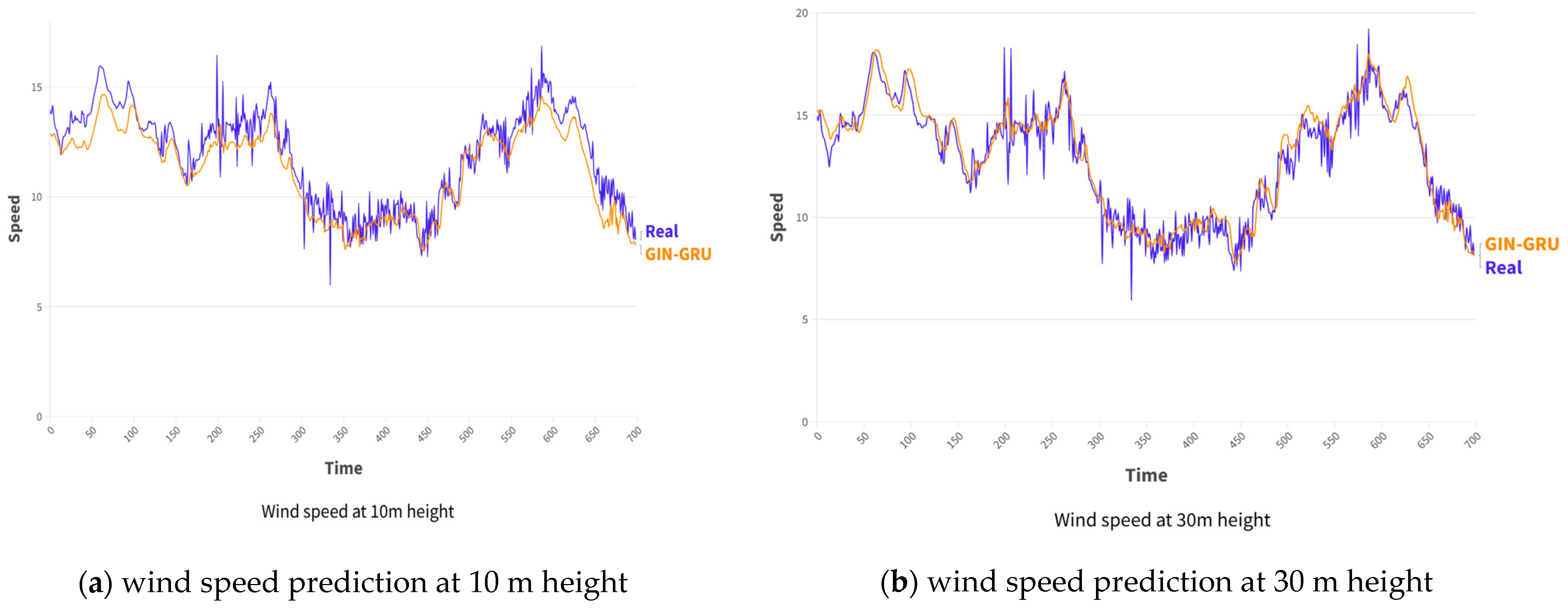
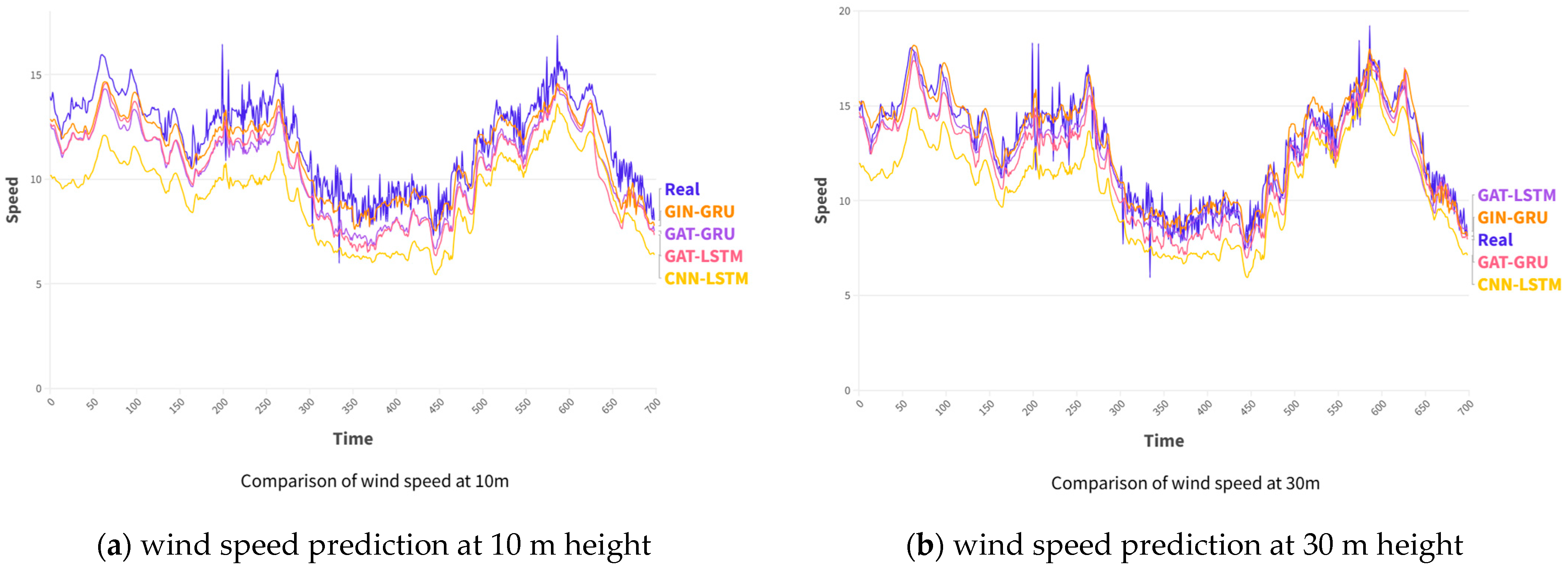
3.2.3. Evaluation and Analysis of GIN-GRU Neural Networks
4. Discussion
4.1. Effect of the Different Nodes on Graph Networks
4.2. Effect of the Different Edges on Graph Networks
5. Conclusions
Author Contributions
Funding
Data Availability Statement
Conflicts of Interest
References
- Valdivia-Bautista, S.M.; Domínguez-Navarro, J.A.; Pérez-Cisneros, M.; Vega-Gómez, C.J.; Castillo-Téllez, B. Artificial Intelligence in Wind Speed Forecasting: A Review. Energies 2023, 16, 2457. [Google Scholar] [CrossRef]
- Chandra, D.R.; Kumari, M.S.; Sydulu, M. A detailed literature review on wind forecasting. In Proceedings of the 2013 International Conference on Power, Energy and Control (ICPEC), Dindigul, India, 6–8 February 2013; pp. 630–634. [Google Scholar] [CrossRef]
- Zhu, C.; Zhu, L. Wind Speed Short-Term Prediction Based on Empirical Wavelet Transform, Recurrent Neural Network and Error Correction. In Journal of Shanghai Jiaotong University (Science); Springer: Berlin/Heidelberg, Germany, 2022; pp. 1–12. [Google Scholar]
- Bokde, N.; Feijóo, A.; Villanueva, D.; Kulat, K. A review on hybrid empirical mode decomposition models for wind speed and wind power prediction. Energies 2019, 12, 254. [Google Scholar] [CrossRef]
- Zhang, Y.; Zhang, C.; SUN, J.B.; Guo, J.J. Improved Wind Speed Prediction Using Empirical Mode Decomposition. Adv. Electr. Comput. Eng. 2018, 18, 3–10. [Google Scholar] [CrossRef]
- Ren, Y.; Suganthan, P.N. Empirical mode decomposition-k nearest neighbor models for wind speed forecasting. J. Power Energy Eng. 2014, 2, 176–185. [Google Scholar] [CrossRef]
- Wang, L.; Liao, Y. A short-term hybrid wind speed prediction model based on decomposition and improved optimization algorithm. Front. Energy Res. 2023, 11, 1298088. [Google Scholar] [CrossRef]
- Qu, Z.; Hou, X.; Hu, W.; Yang, R.; Ju, C. Wind power forecasting based on improved variational mode decomposition and permutation entropy. Clean Energy 2023, 7, 1032–1045. [Google Scholar] [CrossRef]
- Mohapatra, M.R.; Radhakrishnan, R.; Shukla, R.M. A Hybrid Approach using ARIMA, Kalman Filter and LSTM for Accurate Wind Speed Forecasting. arXiv 2023, arXiv:2311.08550. [Google Scholar]
- Che, Y.; Xiao, F. An integrated wind-forecast system based on the weather research and forecasting model, Kalman filter, and data assimilation with nacelle-wind observation. J. Renew. Sustain. Energy 2016, 8, 053308. [Google Scholar] [CrossRef]
- Xu, H.; Chang, Y.; Zhao, Y.; Wang, F. A novel hybrid wind speed interval prediction model based on mode decomposition and gated recursive neural network. Environ. Sci. Pollut. Res. 2022, 29, 87097–87113. [Google Scholar] [CrossRef]
- Ai, X.; Li, S.; Xu, H. Wind speed prediction model using ensemble empirical mode decomposition, least squares support vector machine and long short-term memory. Front. Energy Res. 2023, 10, 1043867. [Google Scholar] [CrossRef]
- Shao, B.; Song, D.; Bian, G.; Zhao, Y. Wind speed forecast based on the LSTM neural network optimized by the firework algorithm. Adv. Mater. Sci. Eng. 2021, 2021, 4874757. [Google Scholar] [CrossRef]
- Zhu, Q.; Chen, J.; Zhu, L.; Duan, X.; Liu, Y. Wind speed prediction with spatio–temporal correlation: A deep learning approach. Energies 2018, 11, 705. [Google Scholar] [CrossRef]
- Trebing, K.; Mehrkanoon, S. Wind speed prediction using multidimensional convolutional neural networks. In Proceedings of the 2020 IEEE symposium series on computational intelligence (SSCI), Canberra, ACT, Australia, 1–4 December 2020; IEEE: Piscataway, NJ, USA, 2020; pp. 713–720. [Google Scholar]
- Tuerxun, W.; Xu, C.; Guo, H.; Guo, L.; Zeng, N.; Cheng, Z. An ultra-short-term wind speed prediction model using LSTM based on modified tuna swarm optimization and successive variational mode decomposition. Energy Sci. Eng. 2022, 10, 3001–3022. [Google Scholar] [CrossRef]
- Yuan, M.M.; Gong, F.M.; Li, X. Multifactor Spatio-Temporal Wind Speed Prediction Based on CNN-LSTM. Comput. Syst. Appl. 2021, 30, 133–141. (In Chinese) [Google Scholar]
- Louppe, G. Understanding random forests: From theory to practice. arXiv 2014, arXiv:1407.7502. [Google Scholar]
- Li, X.; Wang, Y.; Basu, S.; Kumbier, K.; Yu, B. A debiased MDI feature importance measure for random forests. Adv. Neural Inf. Process. Syst. 2019, 32, 713–720. [Google Scholar]
- Abdi, H.; Williams, L.J. Principal component analysis. Wiley Interdiscip. Rev. Comput. Stat. 2010, 2, 433–459. [Google Scholar] [CrossRef]
- Zhou, J.; Cui, G.; Hu, S.; Zhang, Z.; Yang, C.; Liu, Z.; Sun, M. Graph neural networks: A review of methods and applications. AI open 2020, 1, 57–81. [Google Scholar] [CrossRef]
- Waikhom, L.; Patgiri, R. Graph neural networks: Methods, applications, and opportunities. arXiv 2021, arXiv:2108.10733. [Google Scholar]
- Cai, H.; Zheng, V.W.; Chang, K.C.C. A comprehensive survey of graph embedding: Problems, techniques, and applications. IEEE Trans. Knowl. Data Eng. 2018, 30, 1616–1637. [Google Scholar] [CrossRef]
- De Maesschalck, R.; Jouan-Rimbaud, D.; Massart, D.L. The mahalanobis distance. Chemom. Intell. Lab. Syst. 2000, 50, 1–18. [Google Scholar] [CrossRef]
- Leys, C.; Klein, O.; Dominicy, Y.; Ley, C. Detecting multivariate outliers: Use a robust variant of the Mahalanobis distance. J. Exp. Soc. Psychol. 2018, 74, 150–156. [Google Scholar] [CrossRef]
- Goyal, P.; Ferrara, E. Graph embedding techniques, applications, and performance: A survey. Knowl. Based Syst. 2018, 151, 78–94. [Google Scholar] [CrossRef]
- Ju, W.; Fang, Z.; Gu, Y.; Liu, Z.; Long, Q.; Qiao, Z.; Zhang, M. A comprehensive survey on deep graph representation learning. Neural Netw. 2024, 173, 106207. [Google Scholar] [CrossRef] [PubMed]
- Jiang, W. Graph-based deep learning for communication networks: A survey. Comput. Commun. 2022, 185, 40–54. [Google Scholar] [CrossRef]
- Kim, B.H.; Ye, J.C. Understanding graph isomorphism network for rs-fMRI functional connectivity analysis. Front. Neurosci. 2020, 14, 545464. [Google Scholar] [CrossRef]
- Chen, Z.; Villar, S.; Chen, L.; Bruna, J. On the equivalence between graph isomorphism testing and function approximation with gnns. Adv. Neural Inf. Process. Syst. 2019, 32. [Google Scholar]
- Chung, J.; Gulcehre, C.; Cho, K.; Bengio, Y. Empirical evaluation of gated recurrent neural networks on sequence modeling. arXiv 2014, arXiv:1412.3555. [Google Scholar]
- Dey, R.; Salem, F.M. Gate-variants of gated recurrent unit (GRU) neural networks. In Proceedings of the 2017 IEEE 60th international midwest symposium on circuits and systems (MWSCAS), Boston, MA, USA, 6–9 August 2017; IEEE: Piscataway, NJ, USA, 2017; pp. 1597–1600. [Google Scholar]
- Chicco, D.; Warrens, M.J.; Jurman, G. The coefficient of determination R-squared is more informative than SMAPE, MAE, MAPE, MSE and RMSE in regression analysis evaluation. Peerj Comput. Sci. 2021, 7, e623. [Google Scholar] [CrossRef]
- Aykas, D.; Mehrkanoon, S. Multistream graph attention networks for wind speed forecasting. In Proceedings of the 2021 IEEE Symposium Series on Computational Intelligence (SSCI), Orlando, FL, USA, 5–7 December 2021; IEEE: Piscataway, NJ, USA, 2021; pp. 1–8. [Google Scholar]
- Flores, A.; Tito-Chura, H.; Yana-Mamani, V. An ensemble GRU approach for wind speed forecasting with data augmentation. Int. J. Adv. Comput. Sci. Appl. 2021, 12, 569–574. [Google Scholar] [CrossRef]


| Category | Variables |
|---|---|
| Velocity and friction | friction_velocity_2 m |
| Monin–Obukhov length | inversemoninobukhovlength_2 m |
| Roughness | roughness_length |
| Sea temperature | surface_sea_temperature |
| Pressure | pressure_0 m, pressure_100 m, pressure_200 m |
| Humidity | relativehumidity_2 m |
| Precipitation rate | precipitationrate_0 m |
| Wind speed (at various heights) | windspeed_10 m, windspeed_40 m, windspeed_60 m, windspeed_80 m, windspeed_100 m, windspeed_120 m, windspeed_140 m, windspeed_160 m, windspeed_180 m, windspeed_200 m |
| Wind direction (at various heights) | winddirection_10 m, winddirection_20 m, winddirection_40 m, winddirection_60 m, winddirection_80 m, winddirection_100 m, winddirection_120 m, winddirection_140 m, winddirection_160 m, winddirection_180 m, winddirection_200 m |
| Temperature (at various heights) | temperature_2 m, temperature_10 m, temperature_20 m, temperature_40 m, temperature_60 m, temperature_80 m, temperature_100 m, temperature_120 m, temperature_140 m, temperature_160 m, temperature_180 m, temperature_200 m |
| General weather parameters | wind_speed, wind_direction, pressure, temperature |
| Graph Foundation Models | ||||
|---|---|---|---|---|
| ①PS-GIN-GRU | 2.5422 | 1.5944 | 1.4224 | 0.1151 |
| ①GE-GIN-GRU | 0.8457 | 0.9196 | 0.7612 | 0.0636 |
| ② | 2.7184 | 1.6488 | 1.4988 | 0.1231 |
| ②GE-GIN-GRU | 1.0712 | 1.0350 | 0.8645 | 0.0726 |
| ③PS-GIN-GRU | 2.7143 | 1.6475 | 1.4856 | 0.1209 |
| ③GE-GIN-GRU | 0.9258 | 0.9622 | 0.8027 | 0.0685 |
| ④ | 2.7724 | 1.6651 | 1.4912 | 0.1208 |
| ④GE-GIN-GRU | 0.9222 | 0.9603 | 0.7897 | 0.0666 |
| ⑤PS-GIN-GRU | 2.5713 | 1.6035 | 1.4319 | 0.1160 |
| ⑤GE-GIN-GRU | 0.8507 | 0.9223 | 0.7455 | 0.0624 |
| ⑥ | 2.1951 | 1.4816 | 1.3085 | 0.1062 |
| ⑥GE-GIN-GRU | 1.0044 | 1.0022 | 0.8317 | 0.0705 |
| ⑦PS-GIN-GRU | 2.2201 | 1.4900 | 1.3143 | 0.1066 |
| ⑦GE-GIN-GRU | 0.9340 | 0.9665 | 0.8060 | 0.0684 |
| ⑧ | 2.2993 | 1.5163 | 1.3373 | 0.1079 |
| ⑧GE-GIN-GRU | 1.1580 | 1.0761 | 0.9188 | 0.0761 |
| ⑨PS-GIN-GRU | 2.2724 | 1.5074 | 1.3321 | 0.1074 |
| ⑨GE-GIN-GRU | 0.7793 | 0.8828 | 0.7233 | 0.0613 |
| ⑩ | 2.1376 | 1.4620 | 1.2833 | 0.1032 |
| ⑩GE-GIN-GRU | 1.0573 | 1.0283 | 0.8545 | 0.0719 |
| Error Metrics | CNN-LSTM | GAT-GRU | GAT-LSTM | GE-GIN-GRU |
|---|---|---|---|---|
| 7.7851 | 2.1808 | 2.3968 | 0.8457 | |
| 2.7902 | 1.4768 | 1.5482 | 0.9196 | |
| 2.6851 | 1.3567 | 1.4009 | 0.7612 | |
| 0.2283 | 0.1152 | 0.1213 | 0.0636 |
| Error Metrics | CNN-LSTM | GAT-GRU | GAT-LSTM | GE-GIN-GRU |
|---|---|---|---|---|
| 4.9849 | 1.3163 | 1.4214 | 0.6400 | |
| 2.2327 | 1.1473 | 1.1922 | 0.8000 | |
| 2.0489 | 0.9414 | 0.9726 | 0.6076 | |
| 0.1629 | 0.0759 | 0.0787 | 0.0503 |
| Error Metrics | RF | PCA-RF |
|---|---|---|
| 2.5422 | 0.8457 | |
| 1.5944 | 0.9196 | |
| 1.4224 | 0.7612 | |
| 0.1151 | 0.0636 |
| Error Metrics | RF | PCA-RF |
|---|---|---|
| 0.6945 | 0.6400 | |
| 0.8334 | 0.8000 | |
| 0.6354 | 0.6076 | |
| 0.0510 | 0.0503 |
| Error Metrics | GE-GIN-GRU (362) | GE-GIN-GRU (1724) | GE-GIN-GRU (3124) |
|---|---|---|---|
| 1.6184 | 0.8457 | 1.4014 | |
| 1.2722 | 0.9196 | 1.1838 | |
| 1.1254 | 0.7612 | 1.0025 | |
| 0.0924 | 0.0636 | 0.0857 |
Disclaimer/Publisher’s Note: The statements, opinions and data contained in all publications are solely those of the individual author(s) and contributor(s) and not of MDPI and/or the editor(s). MDPI and/or the editor(s) disclaim responsibility for any injury to people or property resulting from any ideas, methods, instructions or products referred to in the content. |
© 2024 by the authors. Licensee MDPI, Basel, Switzerland. This article is an open access article distributed under the terms and conditions of the Creative Commons Attribution (CC BY) license (https://creativecommons.org/licenses/by/4.0/).
Share and Cite
Wu, H.; Chen, H. Multi-Site Wind Speed Prediction Based on Graph Embedding and Cyclic Graph Isomorphism Network (GIN-GRU). Energies 2024, 17, 3516. https://doi.org/10.3390/en17143516
Wu H, Chen H. Multi-Site Wind Speed Prediction Based on Graph Embedding and Cyclic Graph Isomorphism Network (GIN-GRU). Energies. 2024; 17(14):3516. https://doi.org/10.3390/en17143516
Chicago/Turabian StyleWu, Hongshun, and Hui Chen. 2024. "Multi-Site Wind Speed Prediction Based on Graph Embedding and Cyclic Graph Isomorphism Network (GIN-GRU)" Energies 17, no. 14: 3516. https://doi.org/10.3390/en17143516
APA StyleWu, H., & Chen, H. (2024). Multi-Site Wind Speed Prediction Based on Graph Embedding and Cyclic Graph Isomorphism Network (GIN-GRU). Energies, 17(14), 3516. https://doi.org/10.3390/en17143516