Article

A Productivity Prediction Method of Fracture-Vuggy Reservoirs Based on the PSO-BP Neural Network

1
School of Energy Resources, China University of Geosciences, Beijing 100083, China
2
SINOPEC Petroleum Exploration and Production Research Institute, Beijing 100083, China
*
Author to whom correspondence should be addressed.
Energies 2024, 17(14), 3482; https://doi.org/10.3390/en17143482
Submission received: 15 May 2024 / Revised: 4 July 2024 / Accepted: 11 July 2024 / Published: 15 July 2024
(This article belongs to the Section H: Geo-Energy)

Abstract

:
Reservoir productivity prediction is a key component of oil and gas field development, and the rapid and accurate evaluation of reservoir productivity plays an important role in evaluating oil field development potential and improving oil field development efficiency. Fracture-vuggy reservoirs are characterized by strong heterogeneity, complex distribution, and irregular development, causing great difficulties in the efficient prediction of fracture-vuggy reservoirs’ productivity. Therefore, a PSO-BP fracture-vuggy reservoir productivity prediction model optimized by feature optimization was proposed in this paper. The Chatterjee correlation coefficient was used to select the appropriate combination of seismic attributes as the input of the prediction model, and we applied the PSO-BP model to predict oil wells’ production in a typical fracture-vuggy reservoir area of Tahe Oilfield, China, with the selected seismic attributes and compared the accuracy with that provided by the BP neural network, linear support vector machine, and multiple linear regression. The prediction results using the four models based on the test set showed that compared with the other three models, the MSE of the PSO-BP model increased by 23% to 62%, the RMSE increased by 12 to 38 percent, the MAE increased by 18 to 44 percent, the SSE increased by 23 to 62 percent, and the R-square value increased by 2 to 13 percent. This comparison proves that the PSO-BP neural network model proposed in this paper is suitable for the productivity prediction of fracture-vuggy reservoirs and has better performance, which is of guiding significance for the development and production of fracture-vuggy reservoirs.

1. Introduction

Carbonate reservoirs are among the most important hydrocarbon reservoirs in the world. Carbonate oil and gas resources account for approximately 70% of the world’s oil and gas resources, and proven oil and gas reserves account for approximately 50% of the world’s oil and gas resources [1,2], so carbonate reservoirs are important fields for increasing hydrocarbon storage and production. Among carbonate reservoirs, fracture-vuggy carbonate reservoirs are a kind of reservoir group with cavern, solution vuggy, and fracture systems as the main storage space [3]. Because of fracture-vuggy reservoirs’ excellent reservoir performance and good connection of oil sources, they have become a significant research object in relation to exploration and development. Reservoir productivity prediction is a key component of oil development, and the rapid and accurate evaluation of reservoir productivity plays an important role in evaluating oil field development potential and improving oil field development efficiency [4]. Affected by tectonic movement and various diagenesis processes, fracture-vuggy carbonate reservoirs are characterized by strong heterogeneity, complex distribution, and irregular development [5,6], causing great difficulties in the efficient prediction of fracture-vuggy carbonate reservoir productivity. Therefore, it is of great significance to establish a set of fast and accurate productivity prediction models for the further improvement of the development efficiency and recovery efficiency of fracture-vuggy reservoirs.
The existing productivity forecasting methods mainly include the empirical method, analytical formula methods, the numerical simulation method, and artificial intelligence algorithms. The empirical method is a forecasting theory based on oil and gas production data which can be used to establish a regression relationship [7]. Liang et al. realized the prediction of the production level of shale gas reservoirs through the empirical method. Meanwhile, through comparative analysis of 18 models, it was found that although the empirical method is simple and convenient, it is greatly affected by data fluctuations and the flow stage [8]. Niu et al. proposed an empirical model for improved production prediction based on the historical production profile analysis of mass-producing wells [7]. Analytical models are alternative modes of forecasting production [9]. Ozkan et al. considered multi-fractured horizontal wells (MFHWs) with appropriate boundary conditions to highlight the special productivity features of unconventional shale reservoirs [10]. The numerical simulation method can predict the production dynamics of oil and gas wells [11]. Liu et al. developed a novel compositional reservoir model for modeling the production dynamics of gas-condensate wells [12]. Nie et al. put forward a numerical simulation method of discrete cracks embedded in gas reservoirs which improves the efficiency of the application process and can quickly determine the recoverable reserves of wells affected by fracturing [13]. Bi et al. established a 3D directional unsteady well productivity prediction model using the finite-volume method considering the influence of conventional perforation completion parameters, gravel packing perforation completion parameters, natural fractures, reservoir heterogeneity, reservoir scale, skin factor, fluid gravity, fluid compressibility, and rock compressibility [14]. Compared with artificial intelligence methods, analytical formula methods and numerical simulation often need to determine multiple influencing parameters, which is relatively difficult and involves certain uncertainties that affect the prediction accuracy.
Because of their self-learning ability, artificial intelligence algorithms have excellent data analysis and processing ability, and have high accuracy and fault tolerance rates when solving complex logic operations and nonlinear problems [15,16,17,18]. Among these algorithms, machine learning algorithms can automatically learn features from massive and complex historical data and build an evaluation model determined by parameters, in order to make predictions or decisions regarding new inputs [19,20]. The evaluation of reservoir productivity through machine learning has the characteristics of fast calculation speed, strong generalization ability, and accurate results, thus meeting the needs of oil and gas field development and production [21,22]. In recent years, many scholars have tried to predict reservoir productivity with the help of machine learning and obtained high prediction accuracy. Han et al. built a highly robust prediction model with machine learning to achieve the early-stage productivity prediction of shale gas reservoirs [23]. Wang et al. proposed a multi-layer perceptron (MLP) network and a long short-term memory (LSTM) network for shale gas production prediction, providing a fast and effective method for shale gas production prediction [24]. Yuan et al. developed a hybrid deep neural network (HDNN) architecture to predict reservoir production and achieved good prediction results [25]. Abdullayeva et al. proposed a model based on the combination of a convolutional neural network and a long short-term memory network for the prediction of oil production time series [26]. Zhang et al. proposed and verified an oil production prediction method for a single well based on a temporal convolutional network (TCN) [27].
In order to improve the prediction accuracy of fracture- vuggy reservoir productivity, we proposed using the combination of two algorithms to establish a high-precision and high-robustness prediction model. Taking a certain fault-controlled fracture-vuggy reservoir area in Tahe Oilfield, Tarim Basin, China, as the study area, and relying on the seismic attributes and production data of oil wells, a BP neural network improved with the particle warm optimization algorithm was used to create a fracture-vuggy reservoir productivity prediction model, and the prediction performance of this method was compared with that of conventional machine learning algorithm models, providing theoretical support and method references for fracture-vuggy reservoir productivity prediction.

2. Methods

2.1. BP Neural Network Algorithm

The BP neural network model (backpropagation feedforward neural network) is a type of forward feedback learning algorithm put forward by Rumelhant and McClelland in 1986 [28]. As shown in Figure 1, a complete three-layer BP neural network structure can be divided into an input layer, a hidden layer, and an output layer.
The process begins with the data entering the input layer; then, the data are processed by means of weighted summation and an activation function (as shown in Formulas (1) and (2)), propagate forward layer by layer, and finally reach the output layer to obtain the output. The error between the network output and the expected output is propagated backward in some form, and the error is apportioned to each unit. Each layer unit obtains the error signal and uses the error signal as the basis for modifying the weight. This process is repeated until the output reaches the desired value.
Z = i = 1 n x i w i + w 0
y = f ( Z )                     = 1 1 + e Z
where x i and w i represent the i th input value of the node and its weight, respectively, w 0 is the bias value, y is the output of the node, and f is the activation function.

2.2. PSO Algorithm

The particle swarm optimization algorithm (PSO) was first put forward by James Kennedy and Russell Eberhart [29].
v i k + 1 = w v i k + c 1 r 1 p i k x i k + c 2 r 2 g k x i k
x i k + 1 = x i k + v i k
where c 1 and c 2 represent the individual learning factor and the social learning factor, respectively. w is the inertia weight; r 1 and r 2 are random numbers distributed between 0 and 1; and p i k is the individual optimal value of the i th particle after k iterations. g k is the global optimal value after k iterations.
In the PSO algorithm, each candidate solution is treated as a particle, and all particles form a group. Each particle has a velocity (Formula (3)) and position (Formula (4)), the particle moves through space, and a fitness value is associated with that position. Through the exchange of information between individual optimality and global optimality, the optimal position is constantly updated, ultimately maximizing or minimizing the fitness value.

2.3. PSO-BP Algorithm

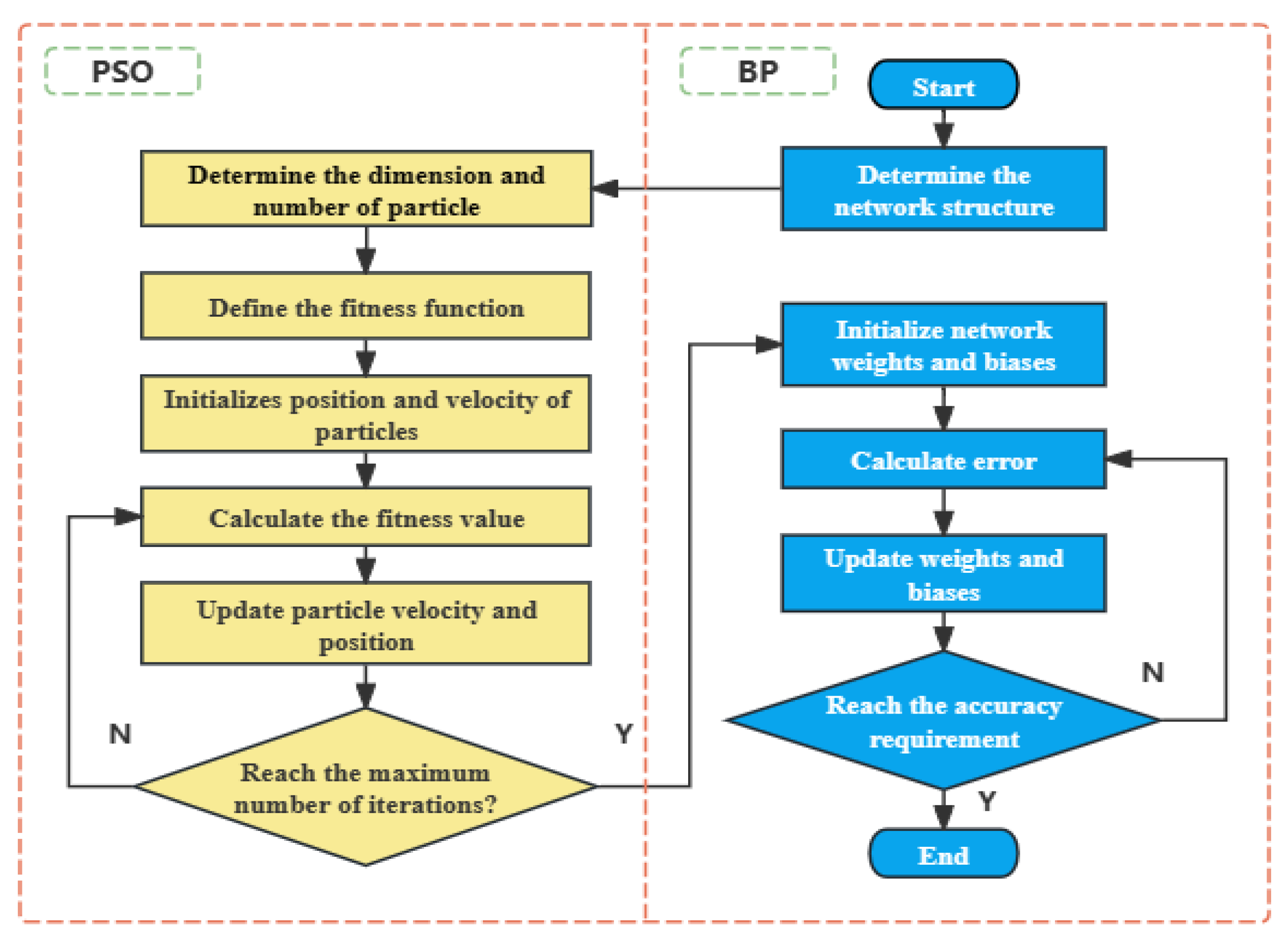
In this study, we proposed a method of fracture-cavity reservoir productivity prediction based on the PSO-BP neural network. The PSO-BP neural network is a neural network model that combines the particle swarm optimization (PSO) algorithm and the backpropagation (BP) algorithm. It uses the PSO algorithm to optimize the weight and bias of the neural network, thereby improving the efficiency of the BP algorithm in neural network training and global search ability. In the PSO-BP neural network, each particle represents a combination of weights and bias parameters for a neural network. These particles move through the search space at a certain speed and update their position based on their individual experience and the experience of their neighbor particles. The updating of the position means the adjustment of the weight and bias of the neural network. Based on this, the BP neural network uses the error backpropagation algorithm to further optimize the network parameters. The workflow of the PSO-BP neural network algorithm is shown in Figure 2. Compared with the traditional BP algorithm, PSO-BP has a stronger global search ability, which can help the neural network to escape the local optimal solution and find the global optimal solution more easily. The PSO-BP algorithm can also effectively use global information to guide the search process, so it usually has a faster convergence rate.
The traditional BP model updates the weight and bias of the neural network by calculating the gradient of the error. However, the gradient descent method can easily be trapped by local changes in gradient within high-dimensional space, especially when the objective function has multiple local minima, causing the BP model to easily fall into the local optimal solution. Additionally, the improper selection of initial weights can also lead to suboptimal solutions, affecting the model’s performance. The PSO algorithm, on the other hand, uses a group of particles (candidate solutions) whose initial positions are randomly distributed. This randomness reduces the model’s dependence on initial weights. Each particle updates its position and velocity based on its own experience and the experience of the best particle in the population. The group renewal mechanism in PSO allows individual particles to fall into local optima while other particles continue the search. The PSO algorithm is self-adaptive, continuously updating the positions and velocities of particles, thereby balancing the search between global and local optima. This makes it more robust across different problems and datasets.
The PSO-BP model combines the global search capabilities of PSO with the local optimization strengths of BP. This hybrid approach not only overcomes the limitations of the BP model by providing a better initial solution, but also uses BP’s efficient local search for fine-tuning purposes. Consequently, the overall performance of the model is improved.

3. Data

3.1. Feature Data

Seismic attributes are special measurements of geometric, kinematic, dynamic or statistical characteristics derived from seismic data, carrying a large amount of reservoir geological information and representing the key information sources for studying and monitoring target reservoirs [30,31,32]. The carbonate fracture-vuggy reservoir is an important oil and gas reservoir space in Tahe Oilfield, Tarim Basin, China [33]. The fracture-vuggy reservoir in this area has remarkable characteristics and abundant high-precision 3D seismic data, providing a sufficient data basis for productivity prediction. Therefore, we chose a certain area of Tahe Oilfield as the study area, and based on the abundant 3D seismic data in this region, we were able to obtain the following attribute data:
  • Distance from fault: During this study, we found that the dissolution cavity and fracture are closely associated, and the high-angle fracture under the unconformity plays an important role in promoting the development of weathering karstification, while the low-angle fracture has a good correspondence with the burial dissolution, and the fault is an important factor affecting the reservoir in the Tahe area. Therefore, we considered the vertical distance between the well location and the fracture as one of the factors affecting the production of wells.
  • Root mean square of amplitude (RMS Amplitude): Because the amplitude value is squared in the process of calculation, it becomes more sensitive to changes in amplitude, and is thus suitable for the analysis of carbonate karst reservoirs.
  • Amplitude change rate: This attribute has a similar effect to the RMS amplitude, and is sensitive to abrupt changes in amplitude in the formation. It can identify the size and scale of karst caverns in carbonate reservoirs, and is thus a key attribute for identifying fracture-vuggy reservoirs.
  • Percentage of frequency attenuation: If porosity has developed in a reservoir and is filled with oil or gas, seismic wave absorption increases, high-frequency absorption attenuation intensifies, and low-frequency energy increases. The frequency attenuation percentage attribute is the percentage of high-frequency attenuation, and is thus widely used in hydrocarbon detection and is sensitive to gas reservoirs.
  • Sweetness: The sweetness value is obtained by the ratio of the instantaneous amplitude of the seismic wave to the instantaneous frequency of the root mean square. Lateral changes in transient amplitudes are usually related to lithology and hydrocarbon accumulation, and the instantaneous frequency can provide information on the effective frequency absorption effect of the seismic event, fracture effects, and reservoir thickness. We can extract the maximum value, minimum value, arithmetic mean value, and geometric mean value of sweetness based on the obtained sweetness value.
  • Beaded area: A fracture-cavity reservoir is mainly characterized by a string of bead-shaped seismic reflections, and the size of the beaded area provides important mapping of a fracture-cavity reservoir product.
We assessed nine attributes of 215 wells in the study area, namely the distance from the fault, the amplitude change rate, the maximum sweetness, the minimum sweetness, the arithmetic mean sweetness, the geometric mean sweetness, the frequency decay percentage, and the beaded area.

3.2. Feature Optimization

In the process of reservoir productivity prediction, various seismic attributes related to reservoir prediction are introduced as the input of the model, but the infinite increase in attributes will have negative effects on reservoir productivity prediction. This is because:
(1)
Some seismic attributes may have nothing to do with the target layer, but reflect the change in interference; if the input attributes are not identified, it will cause confusion, as shown in Figure 3, where there is no clear correlation between some seismic attributes and well production;
(2)
The increase in attributes will bring about computational difficulties, and too much data will take up a lot of storage space and cause a long computation time;
(3)
A large number of attributes will mean that there are a lot of interrelated factors, resulting in duplication and a waste of information.
Figure 3. Crossplots of oil production with the distance from the fault, the amplitude change rate, the maximum sweetness, the minimum sweetness, the arithmetic mean sweetness, the geometric mean sweetness, the frequency decay percentage, and the beaded area.
Energies 17 03482 g003
Therefore, selecting the best seismic attribute subset from the whole seismic attribute set is important in order to reduce the number of solutions and improve the accuracy of reservoir prediction. In this section, feature selection was optimized using the Chatterjee correlation coefficient, and the appropriate attribute combination was selected to predict the oil well production.
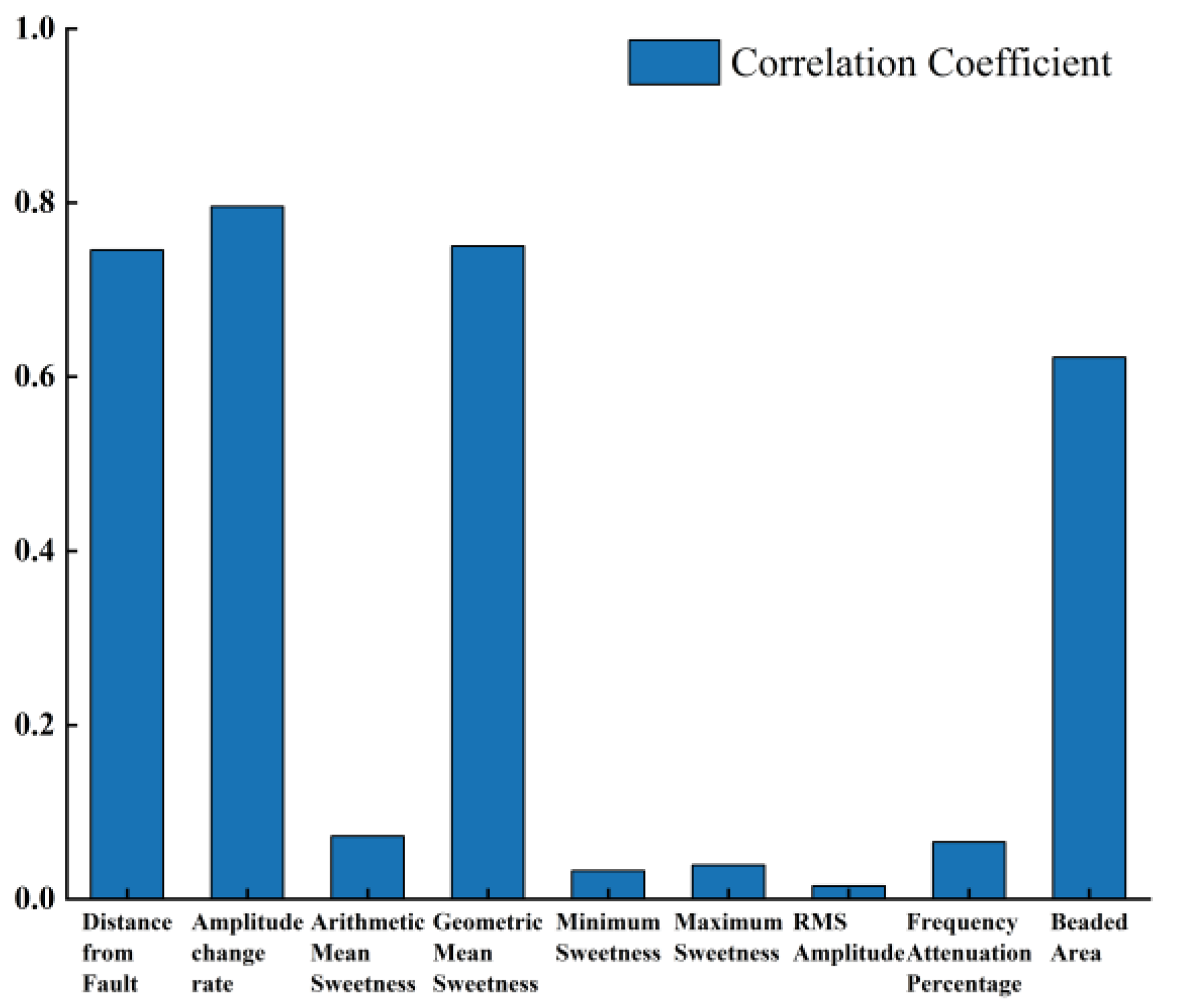
The Chatterjee correlation coefficient (CCC) was proposed by Chatterjee in 2020 [34]; its calculation principle is shown in Equation (5). The distribution range of the Chatterjee correlation coefficient value is between 0 and 1, and the closer the calculation result is to 1, the stronger the correlation between the data. Compared with the conventional correlation coefficient, it can measure not only the linear correlation but also the nonlinear correlation between two kinds of data. We chose the three-month daily oil well production as the metrics of reservoir productivity. The Chatterjee correlation coefficient values between each seismic attribute and well production were calculated. The measurement standard of correlation extent is shown in Table 1, based on which the appropriate attribute combination can be selected as the input feature of the prediction model.
ξ n ( X , Y ) = 1 3 i = 1 n 1 | r i + 1 r i | n 2 1
where X and Y represent the values of the two variables, respectively, r i represents the rank of Y i , and n represents the number of data samples.
The results are shown in Figure 4. It can be seen from this figure that the values of the Chatterjee correlation coefficient of the distance from the fault, the amplitude change rate, the geometric mean value of sweetness, and the beaded area with well production all exceed 0.5, indicating high correlation. Therefore, we chose the four seismic attributes as the model inputs to predict the production of single wells.

4. Results

4.1. Pretreatment

In the course of conducting research on the relationship between dynamic indicators such as the initial production and recoverable reserves of wells and seismic and geological factors, it was found that low-productivity wells and extremely high-productivity wells greatly affected the simulation fitting and prediction accuracy. In order to improve the prediction accuracy, we removed wells with a three-month daily production of less than 10 t/d, and integrated the data of 189 wells for the study.
As the four kinds of seismic attribute data have different value ranges, we normalized the attribute data and three-month daily oil production through Formula (6), so that they were distributed between −1 and 1, in order to accelerate the rate of model convergence.
y = 2 x x min x max x min 1

4.2. Model Setting

In this section, on the basis of the PSO-BP model, we added the traditional linear regression, BP neural network, and SVM-R models as the control group. We compared the fitting effect and prediction accuracy of the three models to illustrate the superiority of model selection. In the experiment, we divided the data (distance from the fault, amplitude change rate, geometric mean value of sweetness, beaded area, and productivity data for 189 wells) based on an 8:2 ratio between the training set and the test set; 38 wells were randomly selected from 189 wells as the test set of the four models, and the other 151 wells were used as the training set of the four models.
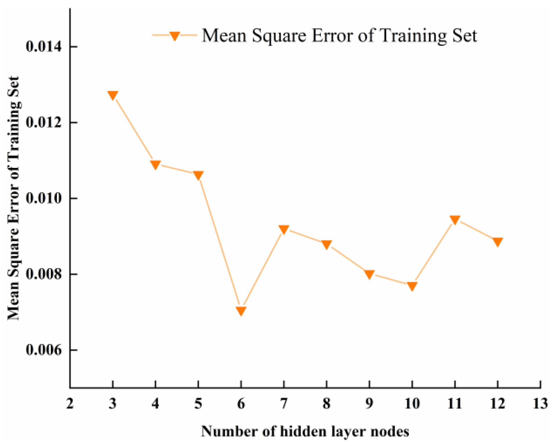
Firstly, we needed to set the hyperparameters of the machine learning model. For the BP neural network, the four neurons in the input layer corresponded to the distance from the fault, the amplitude change rate, the frequency decay percentage, and the beaded area, respectively. The number of hidden layer nodes is a key part of the network structure. Too many nodes will result in slow convergence and will cause overfitting, while too few neurons will cause underfitting. Therefore, according to the theoretical formula (shown in Formula (7)), the number of neurons in the hidden layer was determined to range from 3 to 12, and the training was conducted in each case, after which the mean square error of the training set in each case was calculated using Formula (8), and then the appropriate number of neurons was selected. The test results are shown in Figure 5. Within this interval, when the number of nodes in the hidden layer was six, the mean square error of the training set was the lowest, and so the number of nodes in the hidden layer was determined to be six. The activation function of the hidden layer of the BP neural network was a “Tan-sigmoid” function. For the SVM-R model, a linear function was chosen as the kernel function.
N = m + n + a , a = 1 , 2 , 3 10
where N represents the number of nodes in the hidden layer, m represents the number of nodes in the input layer, and n represents the number of nodes in the output layer.
M S E = i = 1 n ( y i ^ y i ) 2 n
where n represents the number of samples, y ^ represents the predicted value, and y represents the true value.
For the PSO-BP model, the number of neurons in the hidden layer of the PSO-BP network was consistent with that of the BP network, which was set to 6, and each particle was composed of 37 parameters corresponding to the weight of each connection of the neural network and the bias of nodes in the hidden layer and output layer. The individual learning factor and social learning factor were set to 2.0, the population of particles was set to 60, and the maximum number of iterations was set to 800. The upper limit of speed was 1.0 and the lower limit was −1.0. The inertia weight was set to 0.5. The fitness function is defined as the sum of the absolute errors between the predicted value and the true value.

4.3. Productivity Prediction

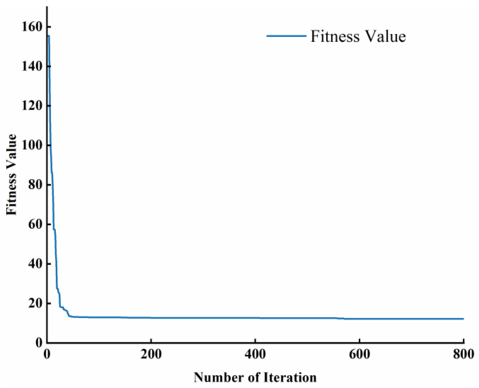
First, we trained the PSO-BP neural network, the BP neural network, the SVM model, and the multiple linear regression model based on the divided training set out in Section 4.2. PSO-BP combines a global search and local tuning, and by calculating and comparing the fitness value under the current parameters, the parameters are continuously adjusted. As shown in Figure 6, the fitness value continuously reduces and finally stabilizes. The parameters at this time are used as the initial parameters of the BP network, and BP is further fine-tuned to obtain the trained PSO-BP model.
After model training, the four models obtained by training were used to predict the test set, and the results are shown in Figure 7. This figure shows the relationship between the predicted results of each model and the actual measured well production in the form of a line graph, and we visualize the absolute value of the residuals of the predicted versus the actual production capacity of the wells under each model in the form of a bar chart in this figure. In Figure 7, (a) is the prediction result of the PSO-BP neural network model; (b) is the prediction result of the BP neural network model; (c) is the prediction result of the SVM-R model; and (d) is the prediction result of the multiple linear regression model. It can be seen from this figure that the error between the predicted value of the PSO-BP model and the actual measured well production is more evenly distributed than that of the other three models, and the absolute error is generally lower than that of the other three models.
To further compare the performance of the four models, we calculated the mean square error (MSE), the root mean square error (RMSE), the mean absolute error (MAE), the sum of squares due to error (SSE), and the coefficient of determination (R-square) between the predicted values and the actual measurement values under the four models. The calculation results are shown in Table 2. For MSE, the PSO-BP model improved by about 23% compared with the BP neural network model, by about 62% compared with the SVM-R model, and by about 38% compared with the multiple linear regression model. For RMSE, PSO-BP improved by about 12% compared with BP, by about 38% compared with SVM-R, and by about 21% compared with the multiple linear regression model. For MAE, PSO-BP improved by about 18% compared with BP, by about 44% compared with SVM-R, and by about 31% compared with the multiple linear regression model. For SSE, PSO-BP improved by about 23% compared with BP, by about 62% compared with SVM-R, and by about 38% compared with the multiple linear regression model. For the R-square value, PSO-BP improved by about 2% compared with BP, by about 13% compared with SVM-R, and by about 5% compared with the multiple linear regression model. It can be seen from the accuracy statistics that all the five accuracy evaluations of the PSO-BP neural network model are higher than those of the other three models; meanwhile, we noticed that the prediction accuracy of the PSO-BP model is greatly improved compared with SVM-R and multiple linear regression, which is because the former can learn and capture the potential nonlinear relationship between the input and output while constructing the linear relationship between the input and output, avoiding a waste of information and learning more fully. Compared with BP, PSO-BP benefits from its superior global search ability, which makes it easier to escape of the local optimal solution and shows better generalization ability. In summary, the prediction accuracy of the PSO-BP neural network model for fracture-cavity reservoir productivity prediction is greatly improved compared with the BP neural network, the SVM-R model, and the multiple linear regression model, and it shows better robustness.

5. Conclusions

In order to further improve the accuracy of the prediction of fracture-cavity reservoir productivity, we took 189 oil wells in a certain area of Tahe Oilfield in China as research objects, analyzed the correlation between relevant seismic attributes and oil well productivity, and proposed a fracture-vuggy reservoir productivity prediction model based on PSO-BP. The main conclusions are as follows.
The Chatterjee correlation coefficient (CCC) was proposed to study the correlation between nine seismic attributes and oil well productivity. With this correlation coefficient, not only the linear relationships between data but also the potential nonlinear relationships between data are taken into account. Through the analysis of correlation value, we chose four high-correlation attributes (distance from the fault, amplitude change rate, geometric mean value of sweetness, and beaded area) as the input of the prediction model. This process can not only eliminate the impact of low-correlation attributes on the accuracy of the model, but can also reduce the input dimensions to improve the operational efficiency of the model.
The PSO-BP productivity prediction model was constructed, and the weight and bias of BP neural network were adjusted by means of particle swarm optimization. We used four seismic attributes as model inputs and oil well productivity as the model output to predict oil well productivity in a certain area of Tahe Oilfield in China. Meanwhile, we compared its prediction accuracy with that of the BP neural network, the SVM-R model, and the multiple linear regression model. The results show that compared with the other three models, the MSE of the PSO-BP model increased by 23% to 62%, the RMSE increased by 12 to 38 percent, the MAE increased by 18 to 44 percent, the SSE increased by 23 to 62 percent, and the R-square value increased by 2 to 13 percent. This comparison showed that the prediction accuracy of PSO-BP was greatly improved.
To sum up, the PSO-BP neural network model proposed in this study is suitable for the prediction of the productivity of fracture-cavity reservoirs and has good performance, which is of guiding significance for fracture-vuggy reservoirs’ development and production.

Author Contributions

Methodology, K.T.; Data curation, Z.K. (Zhihong Kang); Writing—original draft, K.T.; Writing—review & editing, Z.K. (Zhihong Kang) and Z.K. (Zhijiang Kang); Project administration, Z.K. (Zhihong Kang); Funding acquisition, Z.K. (Zhijiang Kang); Formal analysis, K.T.; Software, K.T.; Conceptualization, Z.K. (Zhihong Kang); Supervison, Z.K. (Zhihong Kang); Investigation, Z.K. (Zhijiang Kang); Resources, Z.K. (Zhijiang Kang). All authors have read and agreed to the published version of the manuscript.

Funding

This research was funded by [the Joint Fund for Enterprise Innovation and Development of National Natural Science Foundation of China] grant number [U19B6003]. And the APC was funded by [Zhihong Kang].

Data Availability Statement

The original contributions presented in the study are included in the article, further inquiries can be directed to the corresponding author.

Conflicts of Interest

Author Zhijiang Kang was employed by the SINOPEC Petroleum Exploration and Production Research Institute. The remaining authors declare that the research was conducted in the absence of any commercial or financial relationships that could be construed as a potential conflict of interest.

References

  1. Xu, Z.-X.; Li, S.-Y.; Li, B.-F.; Chen, D.-Q.; Liu, Z.-Y.; Li, Z.-M. A review of development methods and EOR technologies for carbonate reservoirs. Pet. Sci. 2020, 17, 990–1013. [Google Scholar] [CrossRef]
  2. Liang, T.; Hou, J.; Qu, M.; Song, C.; Li, J.; Tan, T.; Lu, X.; Zheng, Y. Flow behaviors of nitrogen and foams in micro-visual fracture-vuggy structures. RSC Adv. 2021, 11, 28169–28177. [Google Scholar] [CrossRef] [PubMed]
  3. Qu, M.; Hou, J.; Qi, P.; Zhao, F.; Ma, S.; Churchwell, L.; Wang, Q.; Li, H.; Yang, T. Experimental study of fluid behaviors from water and nitrogen floods on a 3-D visual fractured-vuggy model. J. Pet. Sci. Eng. 2018, 166, 871–879. [Google Scholar] [CrossRef]
  4. Nwonodi, R.I. A novel model for predicting the productivity index of horizontal/vertical wells based on Darcy’s law, drainage radius, and flow convergence. Heliyon 2024, 10, e25073. [Google Scholar] [CrossRef] [PubMed]
  5. Wang, Y.; Xie, P.; Zhang, H.; Liu, Y.; Yang, A. Fracture-vuggy carbonate reservoir characterization based on multiple geological information fusion. Front. Earth Sci. 2024, 11, 1345028. [Google Scholar] [CrossRef]
  6. He, S.; Chen, B.; Yuan, F.; Wang, X.; Wang, T. Dynamic Reserve Calculation Method of Fractured-Vuggy Reservoir Based on Modified Comprehensive Compression Coefficient. Processes 2024, 12, 640. [Google Scholar] [CrossRef]
  7. Niu, W.; Lu, J.; Sun, Y. An improved empirical model for rapid and accurate production prediction of shale gas wells. J. Pet. Sci. Eng. 2022, 208, 109800. [Google Scholar] [CrossRef]
  8. Liang, H.-B.; Zhang, L.-H.; Zhao, Y.-L.; Zhang, B.-N.; Chang, C.; Chen, M.; Bai, M.-X. Empirical methods of decline-curve analysis for shale gas reservoirs: Review, evaluation, and application. J. Nat. Gas Sci. Eng. 2020, 83, 103531. [Google Scholar] [CrossRef]
  9. Makinde, I.; Lee, W.J. Production Forecasting in Shale Volatile Oil Reservoirs Using Reservoir Simulation, Empirical and Analytical Methods. In Proceedings of the 4th Unconventional Resources Technology Conference, San Antonio, TX, USA, 1–3 August 2016. [Google Scholar]
  10. Ozkan, E.; Brown, M.; Raghavan, R.; Kazemi, H. Comparison of fractured-horizontal-well performance in tight sand and shale reservoirs. SPE Reserv. Eval. Eng. 2011, 14, 248–259. [Google Scholar] [CrossRef]
  11. Arumugham, A.J.; Li, L.; Huang, J.; Luo, C.; Du, F.; Liu, Y.; Ulkhaq, M.M.; Kocisko, M.; Goyal, R.K.; Yusmawiza, W.A.; et al. Study on Productivity Numerical Simulation of Highly Deviated and Fractured Wells in Deep Oil and Gas Reservoirs. In Proceedings of the 2016 The 3rd International Conference on Industrial Engineering and Applications (ICIEA 2016), Hong Kong, China, 28–30 April 2016; Volume 68. [Google Scholar]
  12. Liu, L.; Fan, W.; Sun, X.; Huang, Z.; Yao, J.; Liu, Y.; Zeng, Q.; Wang, X. Gas condensate well productivity in fractured vuggy carbonate reservoirs: A numerical modeling study. Geoenergy Sci. Eng. 2023, 225, 211694. [Google Scholar] [CrossRef]
  13. Nie, J.; Wang, H.; Hao, Y. Rapid productivity prediction method for frac hits affected wells based on gas reservoir numerical simulation and probability method. Open Phys. 2023, 21, 20220233. [Google Scholar] [CrossRef]
  14. Bi, G.; Han, F.; Li, M.; Wu, J.; Cui, Y.; Wang, X. Research on Productivity Prediction Model of Three-Dimensional Directional Wells in Different Reservoirs. J. Energy Eng. 2023, 149, 04023020. [Google Scholar] [CrossRef]
  15. Sircar, A.; Yadav, K.; Rayavarapu, K.; Bist, N.; Oza, H. Application of machine learning and artificial intelligence in oil and gas industry. Pet. Res. 2021, 6, 379–391. [Google Scholar] [CrossRef]
  16. Kuang, L.; Liu, H.; Ren, Y.; Luo, K.; Shi, M.; Su, J.; Li, X. Application and development trend of artificial intelligence in petroleum exploration and development. Pet. Explor. Dev. 2021, 48, 1–14. [Google Scholar] [CrossRef]
  17. Li, H.; Yu, H.; Cao, N.; Tian, H.; Cheng, S. Applications of Artificial Intelligence in Oil and Gas Development. Arch. Comput. Methods Eng. 2020, 28, 937–949. [Google Scholar] [CrossRef]
  18. Kong, X.; Liu, Y.; Xue, L.; Li, G.; Zhu, D. A Hybrid Oil Production Prediction Model Based on Artificial Intelligence Technology. Energies 2023, 16, 1027. [Google Scholar] [CrossRef]
  19. Hajizadeh, Y. Machine learning in oil and gas; a SWOT analysis approach. J. Pet. Sci. Eng. 2019, 176, 661–663. [Google Scholar] [CrossRef]
  20. Fan, Z.; Liu, X.; Wang, Z.; Liu, P.; Wang, Y. A Novel Ensemble Machine Learning Model for Oil Production Prediction with Two-Stage Data Preprocessing. Processes 2024, 12, 587. [Google Scholar] [CrossRef]
  21. Mohamed, A.; Hamdi, M.S.; Tahar, S. A Machine Learning Approach for Big Data in Oil and Gas Pipelines. In Proceedings of the 2015 3rd International Conference on Future Internet of Things and Cloud, Rome, Italy, 24–26 August 2015; pp. 585–590. [Google Scholar]
  22. Ning, Y.; Kazemi, H.; Tahmasebi, P. A comparative machine learning study for time series oil production forecasting: ARIMA, LSTM, and Prophet. Comput. Geosci. 2022, 164, 105126. [Google Scholar] [CrossRef]
  23. Han, D.; Jung, J.; Kwon, S. Comparative Study on Supervised Learning Models for Productivity Forecasting of Shale Reservoirs Based on a Data-Driven Approach. Appl. Sci. 2020, 10, 1267. [Google Scholar] [CrossRef]
  24. Wang, T.; Wang, Q.; Shi, J.; Zhang, W.; Ren, W.; Wang, H.; Tian, S. Productivity Prediction of Fractured Horizontal Well in Shale Gas Reservoirs with Machine Learning Algorithms. Appl. Sci. 2021, 11, 12064. [Google Scholar] [CrossRef]
  25. Yuan, Z.; Huang, H.; Jiang, Y.; Li, J. Hybrid deep neural networks for reservoir production prediction. J. Pet. Sci. Eng. 2021, 197, 108111. [Google Scholar] [CrossRef]
  26. Abdullayeva, F.; Imamverdiyev, Y. Development of Oil Production Forecasting Method based on Deep Learning. Stat. Optim. Inf. Comput. 2019, 7, 826–839. [Google Scholar] [CrossRef]
  27. Zhang, L.; Dou, H.; Wang, T.; Wang, H.; Peng, Y.; Zhang, J.; Liu, Z.; Mi, L.; Jiang, L. A production prediction method of single well in water flooding oilfield based on integrated temporal convolutional network model. Pet. Explor. Dev. 2022, 49, 1150–1160. [Google Scholar] [CrossRef]
  28. Rumelhart, D.E.; McClelland, J.L.; Group, P.R. Parallel Distributed Processing, Volume 1: Explorations in the Microstructure of Cognition: Foundations; The MIT Press: Cambridge, MA, USA, 1986. [Google Scholar]
  29. Eberhart, R.; Kennedy, J. Particle swarm optimization. In Proceedings of the IEEE International Conference on Neural Networks, Perth, WA, Australia, 27 November–1 December 1995; Citeseer: University Park, PA, USA, 1995; pp. 1942–1948. [Google Scholar]
  30. Hampson, D.P.; Schuelke, J.S.; Quirein, J.A. Use of multiattribute transforms to predict log properties from seismic data. Geophysics 2001, 66, 220–236. [Google Scholar] [CrossRef]
  31. Schultz, P.S.; Ronen, S.; Hattori, M.; Corbett, C. Seismic-guided estimation of log properties (Part 1: A data-driven interpretation methodology). Lead. Edge 1994, 13, 305–310. [Google Scholar] [CrossRef]
  32. Zahmatkesh, I.; Kadkhodaie, A.; Soleimani, B.; Azarpour, M. Integration of well log-derived facies and 3D seismic attributes for seismic facies mapping: A case study from mansuri oil field, SW Iran. J. Pet. Sci. Eng. 2021, 202, 108563. [Google Scholar] [CrossRef]
  33. Liu, X.; Yang, J.; Li, Z.; Wang, Y. A new methodology on reservoir modeling in the fracture-cavity carbonate rock of Tahe Oilfield. In Proceedings of the SPE International Oil and Gas Conference and Exhibition in China, Beijing, China, 5–7 December 2006; SPE: Richardson, TX, USA, 2006; p. SPE-104429-MS. [Google Scholar]
  34. Chatterjee, S. A New Coefficient of Correlation. J. Am. Stat. Assoc. 2020, 116, 2009–2022. [Google Scholar] [CrossRef]
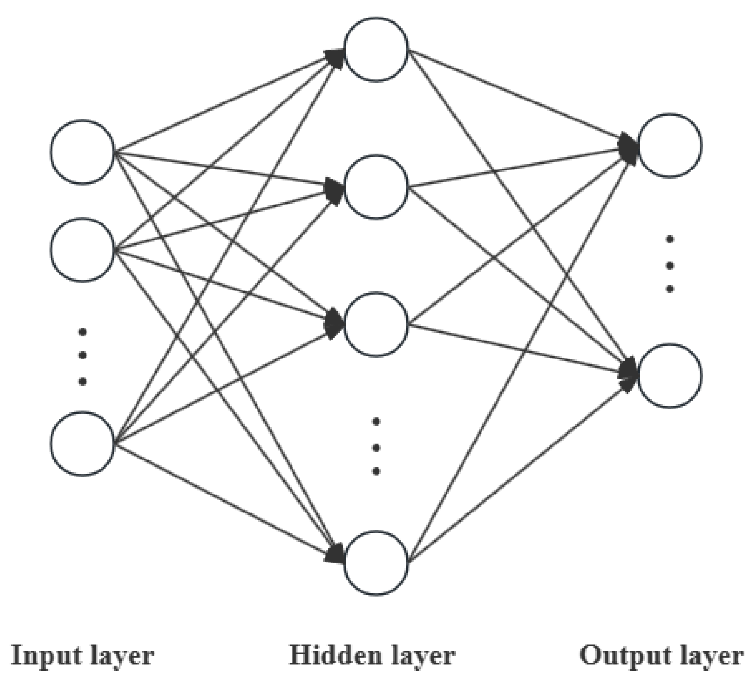
Figure 1. BP network structure.
Energies 17 03482 g001
Figure 2. PSO-BP workflow.
Energies 17 03482 g002
Figure 4. Chatterjee correlation coefficient value between oil production and the distance from the fault, the amplitude change rate, the maximum sweetness, the minimum sweetness, the arithmetic mean sweetness, the geometric mean sweetness, the frequency decay percentage, and the beaded area.
Energies 17 03482 g004
Figure 5. Mean square error of the training set under different hidden layer nodes.
Energies 17 03482 g005
Figure 6. Parameter adjustment process of the PSO-BP model.
Energies 17 03482 g006
Figure 7. Testing results of (a) the PSO-BP model, (b) the BP model, (c) the SVM-R model, and (d) the multiple linear regression model, where the blue line represents the true well production, the orange line represents the model-predicted production, and the green bar represents the absolute residual error between the true and predicted production.
Energies 17 03482 g007
Table 1. Metrics of correlation extent.
Correlation ExtentValue
Non-correlation0.0~0.09
Low-correlation0.1~0.3
Middle-correlation0.3~0.5
High-correlation0.5~1.0
Table 2. Accuracy values of the different models.
MethodMSERMSEMAESSE × 103R-Square
PSO-BP80.58808.97716.41553.06230.9316
BP104.069310.20147.86723.95460.9117
SVM-R209.460214.472711.61047.95950.8223
Linear-Regress128.941511.35529.27374.89980.8906
Disclaimer/Publisher’s Note: The statements, opinions and data contained in all publications are solely those of the individual author(s) and contributor(s) and not of MDPI and/or the editor(s). MDPI and/or the editor(s) disclaim responsibility for any injury to people or property resulting from any ideas, methods, instructions or products referred to in the content.