Article

Influence of Wind and Rainfall on the Performance of a Photovoltaic Module in a Dusty Environment

Faculty of Power Engineering and Power Machines, Technical University of Sofia, 1756 Sofia, Bulgaria
*
Author to whom correspondence should be addressed.
Energies 2024, 17(14), 3394; https://doi.org/10.3390/en17143394
Submission received: 18 April 2024 / Revised: 17 June 2024 / Accepted: 8 July 2024 / Published: 10 July 2024
(This article belongs to the Special Issue Advanced Engineering and Green Energy)

Abstract

:
This study presents an analysis of the influence of weather conditions on the performance of a multicrystalline silicon photovoltaic module, which operates under constant resistive load and is situated near a limestone quarry. The quarry is a significant source of dust, and hence the focus of the study is on the weather factors influencing the presence of soiling on the module’s surface. The analysis encompasses a three-week period, during which the global horizontal irradiance and wind speed were recorded at 10-min intervals by an on-site weather station. The current, voltage, and back temperature of the module were also measured. Supplementary weather data were obtained from the Copernicus Atmosphere Monitoring Service and the NASA POWER databases. The primary objective is to assess whether any influence of the observed weather conditions on the presence of soiling can be inferred from the recorded data. The contribution is in part intended to test how different techniques can be used to extract useful information on the weather-related effects from somewhat limited data, assembled from various sources, while dealing with the underlying uncertainties. The analysis indicates a persistent deterioration of the module’s performance because of soiling and its subsequent improvement due to a favourable weather event.

1. Introduction

The global installed capacity of photovoltaic (PV) systems has experienced rapid growth since the beginning of the century. Starting at just around 385 MW in 2000 [1], it exceeded 1 TW in 2022 [2], and under various scenarios, it is expected to reach approximately 3 TW by 2027 [3], 4.2 TW by 2040 [1], and 4.6 TW by 2050 (equivalent to 16% of projected total power generation) [4]. More ambitious scenarios envisage more than 20 TW [5] and even as high as 30 to 70 TW of installed capacity [6] by 2050. Photovoltaic systems will therefore play a major role in the global energy infrastructure. They also represent one of the most versatile distributed generation technologies, especially considering the advancements in building-integrated photovoltaics [7], the applicability of PV systems in autonomous microgrids [8], and the potential benefits of utilizing the large roofs of commercial and industrial buildings, such as refrigerated warehouses, for on-site power generation [9].
Meanwhile, the integration of PV systems and other renewables in the electricity grid is complicated by their variable output, which is strongly dependent on weather conditions. This volatility represents a significant challenge for grid operators because the electrical grid requires constant balancing of supply and demand, and hence a certain degree of predictability of both. Therefore, as the prevalence of PV systems in the grid increases, reliable prediction of their weather-dependent, intermittent output becomes essential for its management and stable operation [10].
Likewise, reliable prediction of the long-term performance of PV systems, considering in each case the local climate and environment, is one of the crucial factors when selecting appropriate locations for PV facilities. Such long-term assessments should also include the potential impact of future weather variability due to climate change [11] (Other essential considerations include the land requirements and the environmental impact of the projects [12], as poorly selected development sites can threaten biodiversity [13], supplant productive agricultural lands [14], and impact regional water resources [15]). Many studies have thus been dedicated to analysing the effects of different environmental factors on the short-term and long-term performance of PV systems.
When analysing the effects of weather conditions and other environmental factors, it is important to recognize the underlying physical principles that determine the power output of a PV module. The module’s power (P) is the product of current (I) and voltage (V), which at any given time are determined by the I-V characteristics of the module and the connected electric load. Represented graphically, the module operates at the point of intersection of its I-V curve and the I-V curve of the load. Its output thus depends on the connected load and the environmental parameters, which determine the shape of the module’s I-V curve. The latter is a function of solar irradiance ( G T ) and PV cell temperature ( T c ).
For instance, the I-V curves of the module used in this study (which is connected to a constant resistive load, R L = 30 Ω ), calculated at different operating conditions, are shown in Figure 1. For each curve, the highest current (corresponding to zero voltage) is the short-circuit current ( I s c ), the highest voltage (corresponding to zero current) is the open-circuit voltage ( V o c ), and the highest obtainable power corresponds to the rectangle of maximum area under the curve. The current and voltage at that maximum power point (MPP) are denoted as I m p and V m p . Also shown in Figure 1 is the I-V characteristic of the connected constant resistive load ( R L = 30   Ω ). Under most conditions, the point of intersection of the I-V characteristics of the module and the resistive load deviates significantly from the MPP. This is also illustrated in Figure 2.
The two major factors that influence the I-V characteristic of the PV module are solar irradiance and cell temperature. With respect to solar irradiance, it is not only the total amount that matters, but also its spectral distribution and the angle of incidence [16]. Only photons with energy equal to or higher than the semiconductor’s band-gap energy can promote electrons from the valence band to the conduction band and thereby activate charge carriers (electron-hole pairs) in a PV cell. Absorbed photons with lower energy (and thus higher wavelengths) do not activate charge carriers but instead increase the temperature of the semiconductor. Because a single photon can promote a single electron in the conduction band—i.e., it can create only one hole-electron pair—a photon’s energy in excess of the semiconductor’s band-gap energy is also not utilized for the generation of electricity. This excess energy is likewise converted to thermal energy within the material.
Therefore, in semiconductors with band-gap energies of 1.1 to 1.4 eV (such as silicon), a maximum of about 45% of incident solar radiation could be useful for activating charge carriers [17], while much of the remaining energy only contributes to raising the cell temperature. The maximum useful irradiance is dependent on the spectral distribution—changes in the spectral distribution affect the amount of photons at different wavelength bands and thus the total amount of energy that can be utilized for the photovoltaic effect. The spectral distribution is dependent on the composition of the atmosphere (including the humidity ratio), the solar zenith angle, the presence of clouds, and other factors [16,18]. Meanwhile, the angle of incidence of solar radiation has influence on the reflectance of a PV module’s surface and hence on the amount of radiation absorbed by the cell.
With other limitations also considered, the maximum theoretical efficiency of a PV cell is much lower than the aforementioned maximum useful irradiance. For a crystalline silicon PV cell, the theoretical limit is approximately 33%, while the highest experimentally measured efficiencies are around 25% [17,19].
When the temperature of a PV cell increases, this generally reduces the band-gap energy of the semiconductor and raises the intrinsic carrier concentration, thereby affecting the open-circuit voltage ( V o c ) [20,21]. Ultimately, the impact of an increased temperature on the I-V characteristic of the PV module is a slight increase in the short-circuit current ( I s c ) (as a result of the greater number of activated charge carriers at the lower band-gap energy), but a much more significant decrease in the open-circuit voltage ( V o c ) [22].
Considering the typical shape of the I-V curve of a crystalline silicon PV module (see Figure 1), this has an insignificant effect on power output at lower voltages but can lead to a significant reduction in power when the voltage is near to or above that at the maximum power point ( V m p ). All factors that influence the temperature of the semiconductor are hence important for the module’s efficiency. These factors are determined from the energy balance, which incorporates the absorbed solar radiation and the convective and radiative heat flows.
By recognizing the aforementioned physical principles, the major environmental factors that influence the performance of PV modules can be summarized in the following categories:
  • Factors that immediately affect the total amount, incidence angles, and/or spectral distribution of solar radiation reaching the semiconductor, e.g., shading, clouds, aerosol particles, humidity, surface soiling or wetness, etc.
  • Factors that have effect on the deposition, retention, accumulation, and cementation of soiling particles on a module’s surface (and thereby influence the fraction of incident radiation absorbed by the cell), including wind, precipitation, relative humidity, air temperature, etc.
  • Factors that influence cell temperature via heat transfer, such as wind, precipitation, and air temperature (Many studies have investigated the effect of wind, including some considering the local variations in module temperature [23,24]. Typically, higher wind speed results in enhanced heat transfer and a reduction in the temperature of the module, which is beneficial for its power output. However, contrary results have also been reported as a consequence of uneven cooling [25]. In addition to wind speed, wind direction has also been considered as an important factor [26,27], for it determines the windward side of the module and the development of the boundary layers. Nevertheless, in some studies its effect has been found to be rather small or insignificant [28,29]).
  • Factors leading to long-term material degradation, such as gradual moisture ingress [30,31], mechanical damage due to extreme weather events [32,33], and soiling, which can induce lasting material degradation in PV modules via the effects of surface abrasion and uneven heating [34].
Many recent contributions have focused specifically on the impact of soiling, which can be caused by dust or multiple other pollutants, ranging in size from small particles of various types (1 μ m to 500 μ m) [3]—including limestone particles [35,36,37,38,39,40]—to larger objects, such as bird droppings [41], biofilms, plant debris [42], or mud drops. This interest is understandable because soiling is among the major concerns for the maintenance and efficient operation of PV systems [42]. It is not uncommon for locations that are otherwise suitable for solar power generation, i.e., sites with abundant solar radiation, to be in dusty environments and/or prone to experiencing severe dust storms [4,43]. Suitable examples include deserts, as well as arid regions in Asia and Africa with substantial anthropogenic air pollution, where multiple studies have shown that dust accumulation can lead to a significant reduction in PV power output [42,44].
Both the presence of dust in the atmosphere and dust deposition on the surfaces of PV panels are important factors, but the latter typically has a much more significant negative effect [4]. Various publications demonstrate that in the absence of regular cleaning, the efficiency of PV modules in dusty environments can be reduced by more than 50% [4].
Rainfall is an important natural cleaning mechanism, which, in sufficient amounts and intensity, can alleviate the issue of soiling [42]. However, it has been found to be much more efficient in washing off larger particles (e.g., polen) rather than smaller dust particles (of sizes less than 10 μ m) [45]. Furthermore, some of the accumulated soiling may not be carried away entirely and stick to the lower parts of the module’s surface [46]. Naturally, the washing effect is more significant when the rainfall is heavier, continuous, and more prolonged [47,48]. In spring and summer, precipitation can also benefit PV performance via the effects of cooling and reduction of reflection losses [49].
Meanwhile, the deposition, retention, and accumulation of soiling particles on the surfaces of PV modules is also influenced by weather factors, such as humidity, wind, and air temperature. Wind can be either beneficial or detrimental—although it can carry away particles from a given surface by rolling, sliding, or lifting them off [50], depending on their size [51], it can also disperse dust in the atmosphere and afterwards bring about its deposition on the surface [52]. Like rainfall, wind has been found to be an efficient cleaning mechanism predominantly for larger particles, as very large sheer velocities are required to detach smaller ones [53].
Precipitation and humidity can also promote the deposition, adhesion, and coagulation of soiling particles on a PV module’s surface [54,55]. For instance, rain can have a negative effect if it is very light or too brief—it can collect particles dispersed in the atmosphere, deposit soiling on the module’s surface, fail to wash this soiling off, and ultimately leave large dirt spots on the surface afterwards [44]. Moisture can also promote adhesion by inhibiting the rebound of soiling particles from the surface [56]. The problem is compounded in locations with simultaneously high levels of dust and humidity, where the combination of surface moisture (e.g., arising from dew or light rain), dust deposition, and sunlight can lead to cementation of the accumulated soiling [44]. In the aftermath, the surface of the module becomes difficult to clean even by artificial means [56].
Although soiling often represents a major cause for suboptimal performance of PV systems, in many cases its effect can be underestimated or remain unnoticed due to a lack of monitoring. Considering the growing importance of PV technologies in the global energy infrastructure, much value can be brought to their operators and to the infrastructure as a whole by proper monitoring and the development and advancement of predictive maintenance tools, incorporating machine learning models [57,58,59], capable of forecasting and detecting the effect of soiling [60]. This will ensure the proper scheduling of maintenance activities, through which soiling is dealt with effectively and efficiently.
The present study aims to contribute to the body of knowledge underlying the development of such predictive maintenance tools. It presents an analysis of the influence of weather conditions on the performance of a multicrystalline silicon (mc-Si) photovoltaic module, which operates under constant resistive load and is situated near a fairly significant source of limestone dust at a location in Bulgaria.
The primary objective of the study is to assess whether any influence of the observed weather conditions on the presence of soiling on the module’s surface can be inferred from the recorded data by the application of various machine learning models. This objective is motivated by the relatively high levels of dust pollution in the vicinity of the module. In light of the aforementioned previous research, emphasis is placed on the influences of wind and precipitation. The contribution is in part intended to test how different techniques can be used to extract useful information on the weather-related effects from somewhat limited data, assembled from various sources, while dealing with the underlying uncertainties.
The presented analysis reveals that a persistent deterioration of the PV module’s performance as a result of soiling and its subsequent improvement due to a favourable weather event can be detected on the basis of the available data. The study illustrates the difficulties and uncertainties that may arise when dealing with field data and provides some insight into how these issues may be approached to extract meaningful information.

2. Materials and Methods

The PV module under investigation is made of 36 mc-Si cells and has the following electrical characteristics at standard test conditions ( G T = 1000 W m 2 , T c = 25 °C air mass 1.5 spectrum): V m p = 18.2 V, I m p = 1.12 A, V o c = 22.6 V, I s c = 1.18 A. The I-V characteristics of the module at different operating conditions, as shown in Figure 1, were obtained via the six-parameter single-diode model (SDM) [61,62], implemented in PVLIB-Python [63,64].
According to this model, the I-V curve of the module at given irradiance and cell temperature is determined from the single diode equation:
I = I L I o e V + I R s a 1 V + I R s R s h ,
where I L is the light-generated current, i.e., photocurrent (A), I o is the diode reverse saturation current (A), R s is the series resistance ( Ω ), R s h is the shunt resistance ( Ω ), and the parameter a is the product of the diode ideality factor, the number of cells in series, and the cell thermal voltage (V), which in turn is calculated as the product of the Boltzmann’s constant and cell temperature, divided by the electronic charge. These parameters are determined on the basis of their values at reference conditions (five parameters), along with a sixth parameter, called Adjust [61,62].
The six parameters are estimated from the module’s electrical characteristics at standard test conditions and the module’s temperature coefficients for short-circuit current, open-circuit voltage, and maximum power (The temperature coefficients from the module’s datasheet are shown in Table 1). The current-voltage curve of the PV module is determined from these parameters along with the given global in-plane irradiance and cell temperature.
The PV module was mounted on a frame at a 30-degree slope and facing 6 westwards from due south. It was situated near a dust-emitting source, i.e., a limestone quarry, at a location in southwestern Bulgaria. The analysis herein encompasses a period of 21 days in the month of September (2021), during which the global horizontal irradiance (GHI) and wind speed were recorded by an on-site weather station. Wind speed was measured by a rotating cup anemometer, while the pyranometer for measuring GHI is with a silicon photovoltaic detector.
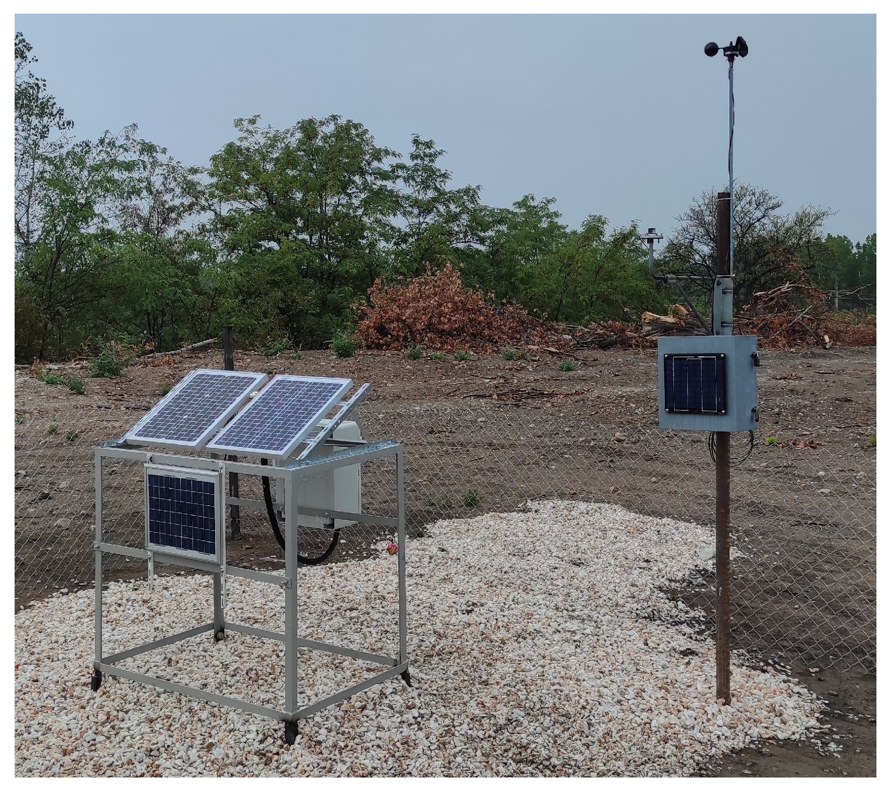
The current, voltage, and back temperature of the module were also measured. The latter was calculated as the average of the measurements of 9 sensors, attached at different points on the back surface. The on-site measurements were recorded at 10-min intervals, wherein the recorded value is the average of the measurements taken each second. The test site is shown in Figure 3.
Supplementary hourly weather data, including air temperature, relative humidity, barometric pressure, wind direction, and precipitation, were obtained from NASA’s POWER database [65]. In addition, GHI data at one-minute intervals were obtained from the Copernicus Atmosphere Monitoring Service (CAMS) [66,67,68,69,70].
Both datasets were resampled at ten-minute intervals to match the recorded datapoints. Since the CAMS dataset has higher frequency than the on-site measurements, it was downsampled (via averaging), while the lower frequency time series from NASA’s POWER database were upsampled (via interpolation). The CAMS dataset was used as a point of reference when analysing the irradiance measured by the weather station.
The following features were calculated for each datapoint (10-min period):
  • The average power of the module was calculated from the measured voltage.
  • The global in-plane irradiance was calculated from the measured GHI using the HDKR (Hay-Davies-Klucher-Reindl) model [61]. The diffuse fraction of GHI was estimated according to the model of Erbs et al. [71], while the relative air mass was determined from the apparent zenith angle [72].
  • The current-voltage curve of the PV module was determined according to the aforementioned PVLIB-Python implementation of the six-parameter SDM based on the calculated global in-plane irradiance and the measured average back temperature of the module. The theoretical power output of the module was obtained via an optimization algorithm, which finds the voltage (and thus power) on the given curve corresponding to the connected constant resistive load ( R L = 30 Ω ) (In essence, the algorithm finds the intersection of the two curves—that of the module and that of the load).
The fixed resistive load has obvious disadvantages and is not representative of the majority of PV systems. As shown in Figure 2, it is clear that the given configuration usually produces considerably lower than the optimal power, which is especially pronounced at higher irradiation levels. Moreover, when the irradiance is higher than about 600 W m 2 the gradient of the power curve becomes very steep. This has to be remarked in the context of the study.
Nevertheless, this configuration benefits from its simplicity and inexpensiveness, and in previous studies it has been shown to be a viable option for monitoring long-term PV performance when the resistance is properly chosen [73]. In the given case, the connected resistance load is not optimal but was nonetheless considered suitable for the purposes of the analysis (even though it is not the best option).
One particular advantage of this configuration is that part of the time the power output of the PV module is essentially independent of temperature. This happens when the irradiance is relatively low (below about 400 W m 2 ), wherein the I-V characteristics of the module and the load intersect at voltages below approximately 15 V. As shown in Figure 1 and Figure 2, under such conditions the current-voltage and thus the power-voltage curves of the PV module at a given irradiance but different cell temperatures are almost overlapping (these curves begin to diverge significantly when the voltage exceeds 15 V). Therefore, temperature-related effects on the module’s power output are not relevant for the corresponding datapoints.
In addition to PVLIB (0.10.1), various Python (3.11) libraries were used for analysing the data, including NumPy (1.24.2) [74] for array and matrix operations; pandas (1.5.3) [75,76,77] for dataframe operations (including resampling); Matplotlib (3.7.0) [78] and seaborn (0.12.2) [79] for data visualization; SciPy (1.10.0) [80] for computing smoothing splines [81]; statsmodels (0.14.0) [82] for seasonal-trend decomposition using locally estimated scatterplot smoothing (LOESS) [83]; and Scikit-learn (1.2.2) [84] for principal component analysis (PCA) [85].
The Pearson correlation coefficient [10,86] has been used as a measure of the linear correlation between the variables. Hence, values close to 1 indicate a strong positive linear correlation, whereas values close to 1 indicate a strong negative linear correlation.

3. Results and Discussion

3.1. General Observations

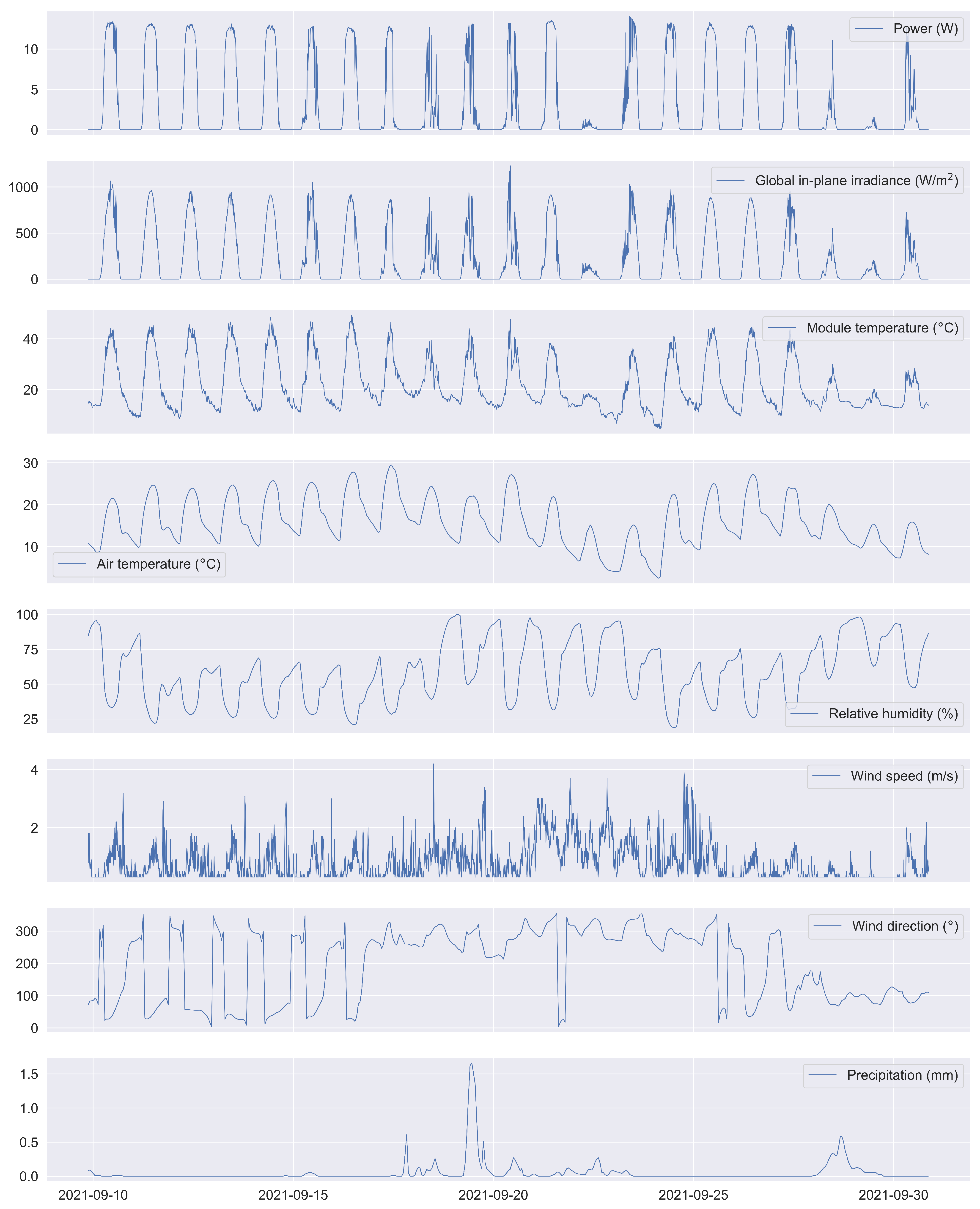
The original time series data on which the analysis is based are shown in Figure 4.
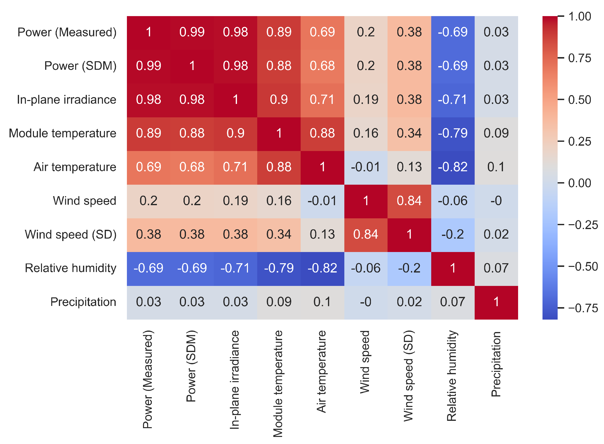
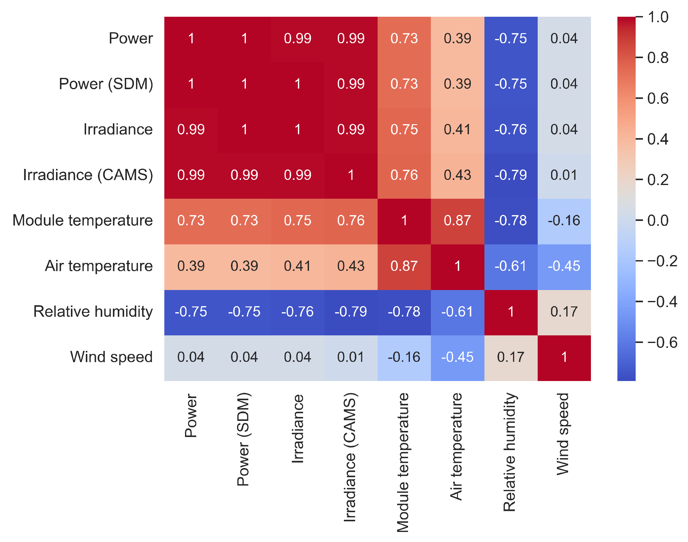
Predictably, some of the features are highly correlated, as shown in Figure 5. In addition to the variables from Figure 4, also shown are the power calculated according to the SDM as well as the standard deviation (SD) of measured wind speed.
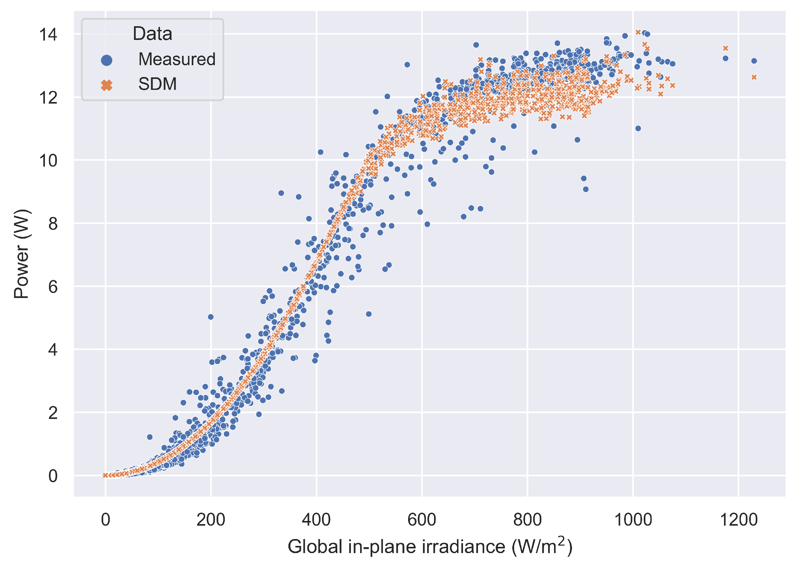
As should be expected, the module’s power (both measured and calculated) is strongly correlated with the global in-plane irradiance in the first place and the module’s back temperature in the second place. The latter is highly correlated with the irradiance, air temperature, and, to a lesser degree, wind speed. The negative correlation of power and module temperature with relative humidity is associated with the inherent negative correlation between air temperature and relative humidity. A high correlation between the average wind speed and its standard deviation is expected, as higher average wind speed is associated with stronger wind gusts. The strong correlation between power and irradiance is shown in Figure 6.
The power nearly evens out at high irradiance levels because of the constant resistive load (see Figure 2), which leads to continually decreasing efficiency. This effect is also captured well by the SDM, although it consistently underestimates the power output at irradiances above approximately 600 W m 2 , i.e., when the operating point is to the right of the MPP. This is the part of the I-V curve where the derivatives of current and power with respect to voltage are large, i.e., a small change in voltage results in a sharp change in current and power. As observed in previous studies, this is where the single diode models are less accurate [87].
Furthermore, this is also where the temperature coefficients used in the model have the most significant impact. These coefficients can often be determined inaccurately and with significantly underestimated uncertainty [88]. Indeed, it was observed that the same coefficients, specified for the given module, were provided in the datasheets of other PV modules of the same manufacturer too. Therefore, the values in Table 1 are dubious and may not be accurate. This is an important consideration when conducting comparisons between measured and modelled PV power output. Such issues should not be confused with deficiencies in the predictive capabilities of the model or the quality of the other data involved.
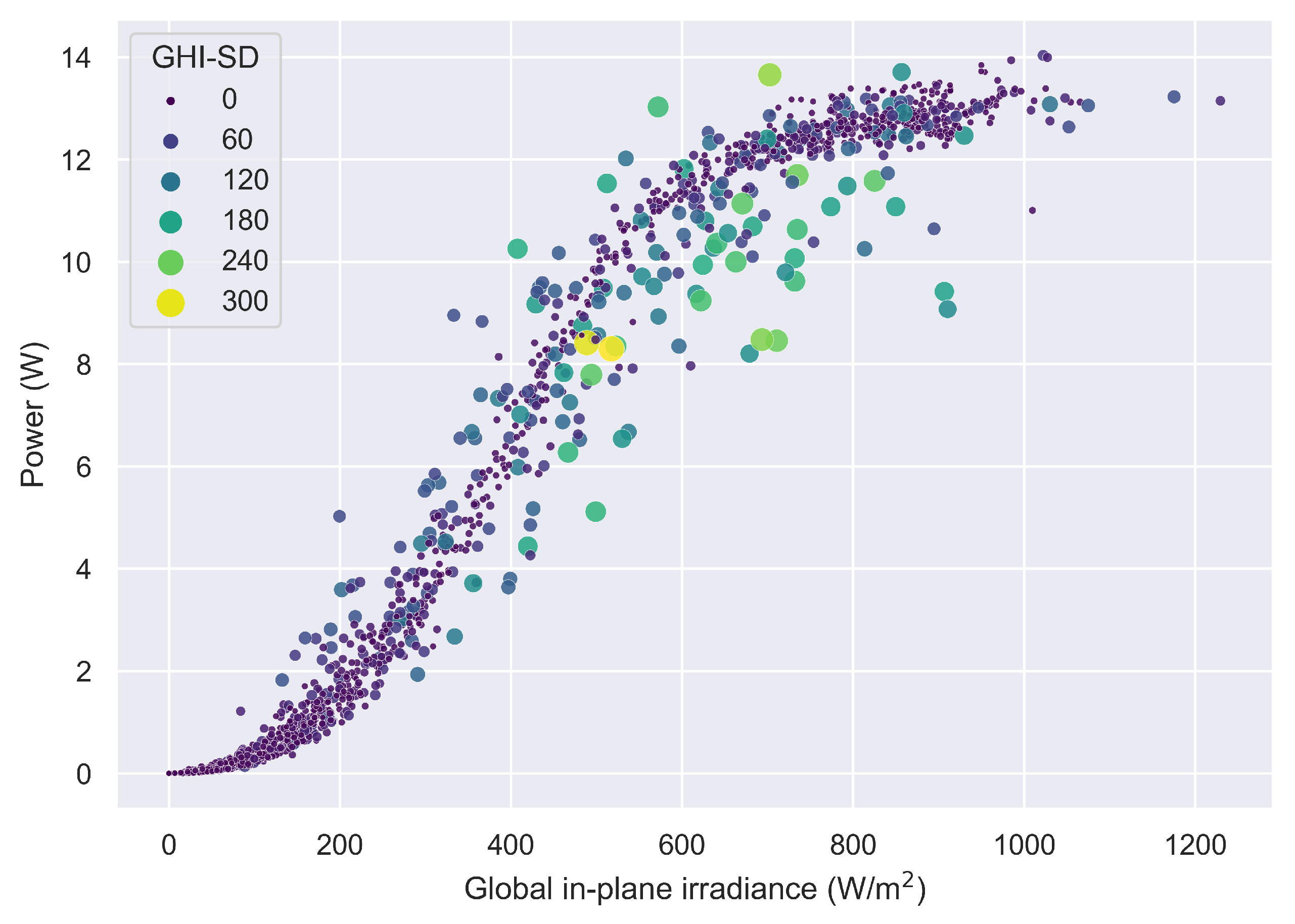
Considering all the uncertainties involved, the module prediction corresponds relatively well with the measurements. An additional point to clarify is the presence of outliers, i.e., the measured points deviating significantly from the model, and whether they could be attributed to some weather effect. As shown in Figure 7, almost all of these datapoints correspond to 10-min intervals with a very high standard deviation of the measured GHI. Therefore, they could be more likely attributed to errors arising from time-averaging, rather than to any other significant effect.
It is important to identify an additional source of uncertainty, which is associated with the GHI measurements of the weather station’s pyranometer. Field measurements of solar irradiance also suffer from the soiling issues affecting PV modules and can thus underestimate the measured irradiation [89]. This can further lead to underestimation of the soiling losses of the PV module [90,91].
Indeed, the comparison between the GHI measured by the on-site pyranometer and the dataset obtained from CAMS shows that the former is consistently lower, except for the first day of measurements. This is illustrated in Figure 8 and Figure 9. The observed tendency indicates that the pyranometer’s surface has been soiled soon after the installation of the weather station and is therefore expected to underestimate the irradiance.

3.2. Principal Component Analysis and Change Detection

Since some of the features in the weather data are highly correlated, it is appropriate to apply a technique for obtaining a smaller number of decorrelated features, explaining the variabilities of the weather. This can help to avoid misinterpretations of the individual influence of each weather parameter and allow for better understanding of their combined effects.
A suitable method is principal component analysis (PCA). It produces new variables, called principal components (PC), which are uncorrelated linear combinations of the original ones [85]. The original variables are first standardized (such that each has a zero mean and unit variance), forming the matrix X. In this case, the matrix contains six columns, corresponding to the global in-plane irradiance, air temperature, relative humidity, wind speed, wind direction, and precipitation. The principal components are then determined from the singular value decomposition of X:
X = U D V T ,
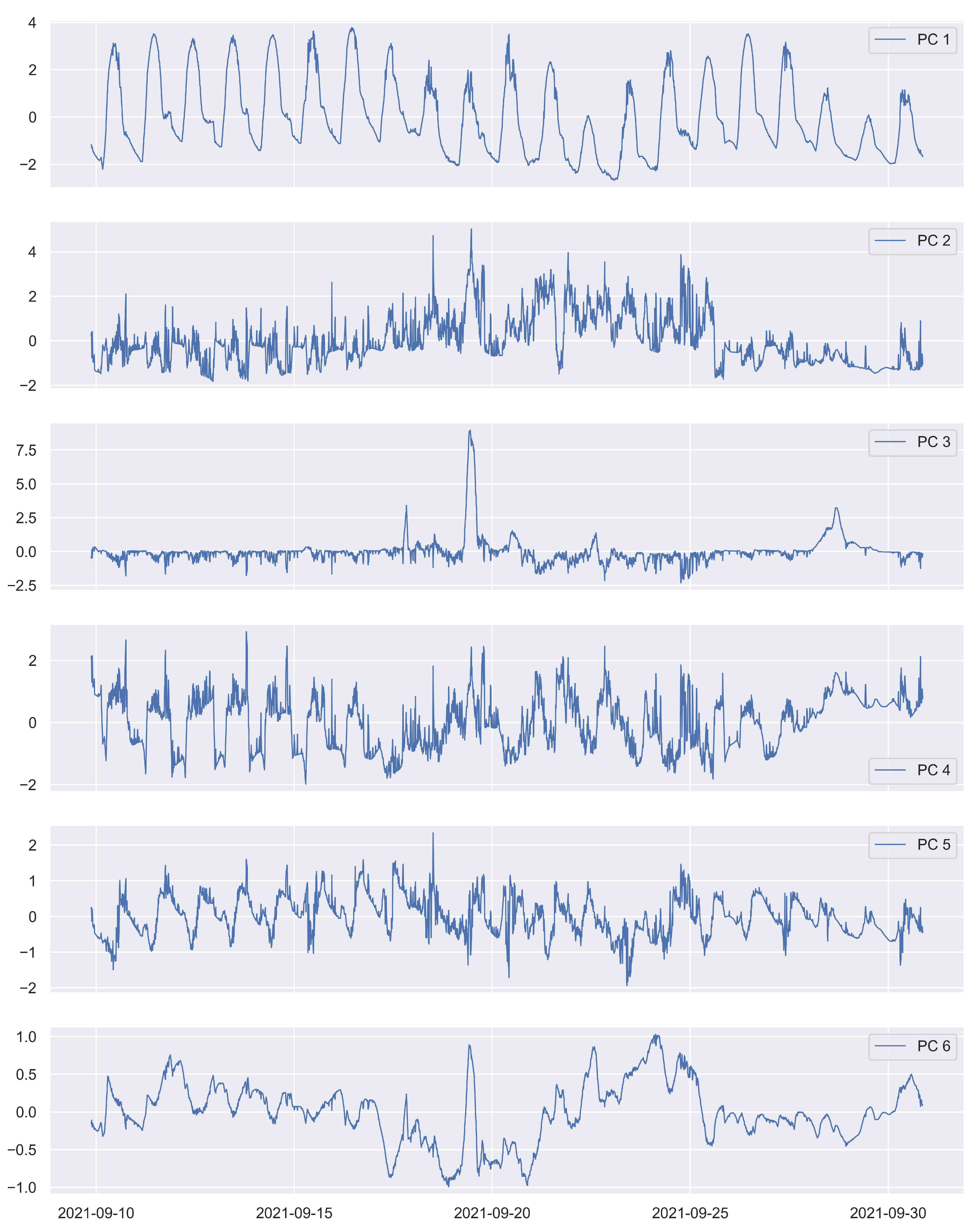
where D is the diagonal matrix of singular values, while U and V are the ortogonal matrices containing the left and right singular vectors. The columns of U D are the principle components of X (Because these columns are orthogonal vectors, they are uncorrelated). The PCs obtained in this manner are shown in Figure 10.
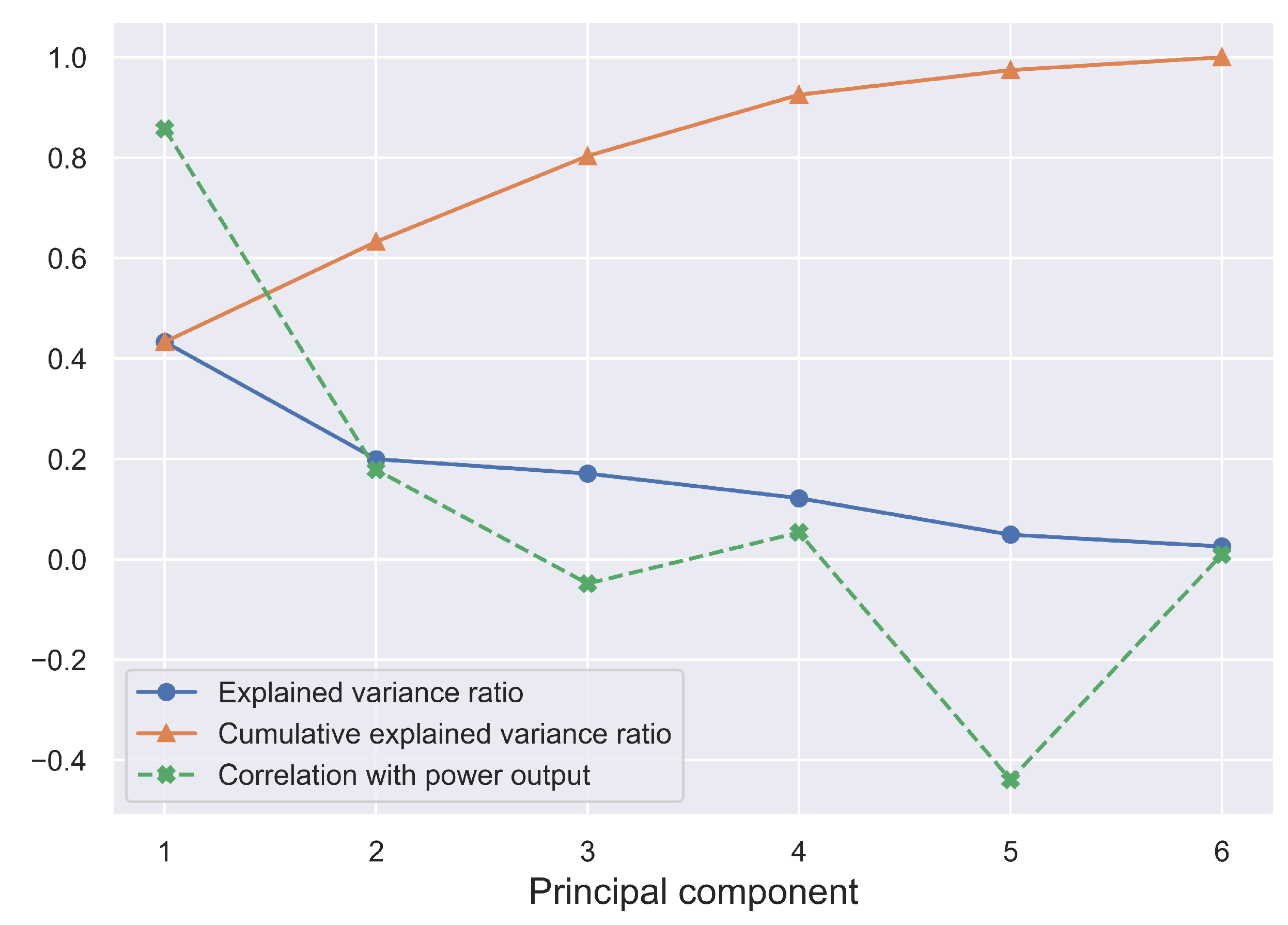
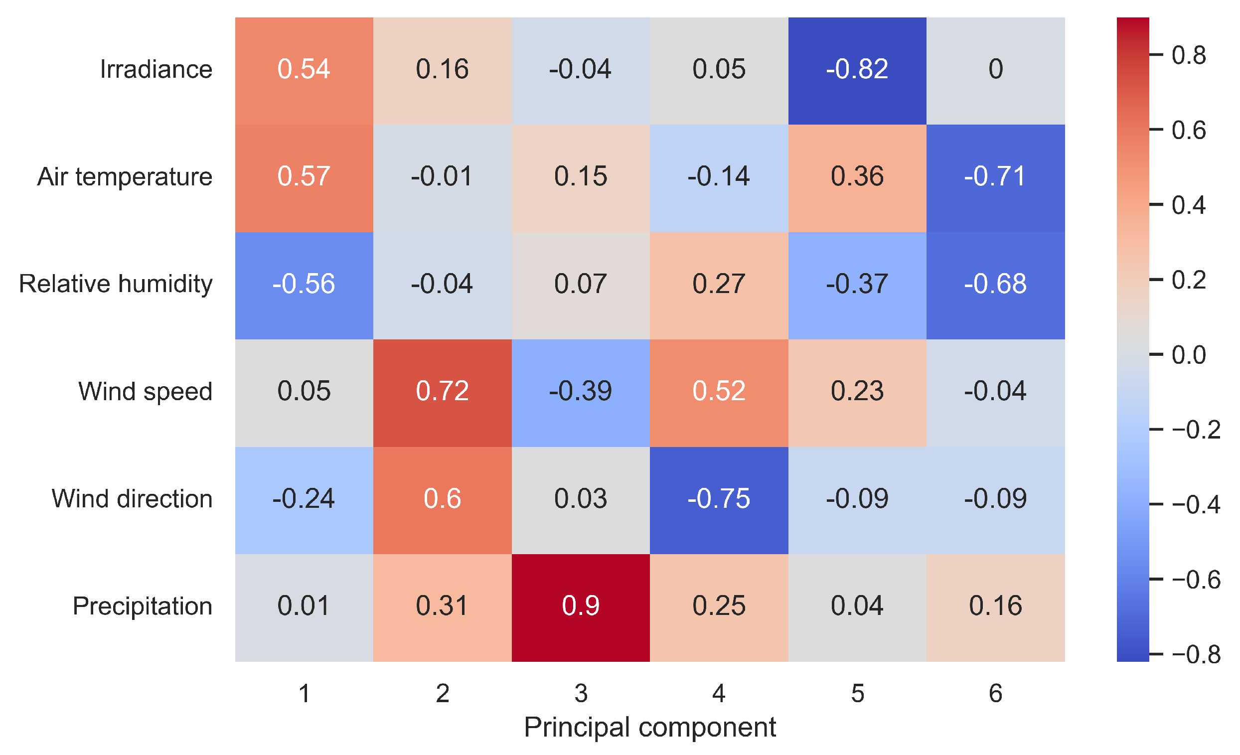
The singular vector with the highest corresponding singular value captures the greatest share of the variance in the original data. The columns of the orthogonal matrices are arranged such that each consecutive PC explains a smaller share of the variance. The variance explained by a principal component is equal to the square of the corresponding singular value, divided by the degrees of freedom (the number of samples minus 1). The explained variance ratios are the scaled explained variances, such that their sum equals one [85]. The explained variance ratios are shown in Figure 11. Also shown is the Pearson correlation coefficient of each PC with the power output of the PV module. The correlations of the PCs with the original weather variables are shown in Figure 12.
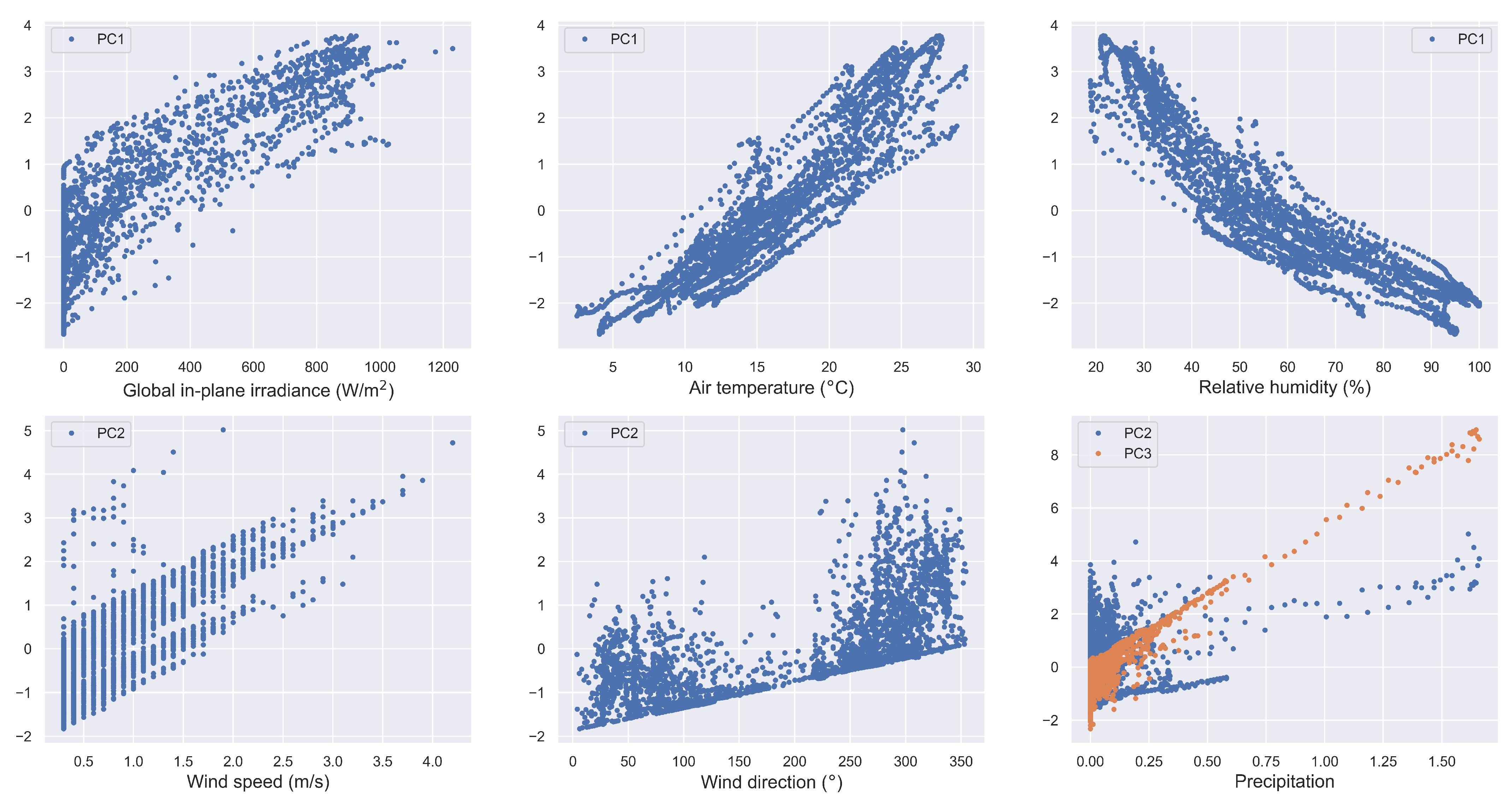
Most of the variance in the original data is explained by the first four PCs, with the first three capturing 80% of the total. The correlation map clearly shows that the first PC, which is strongly correlated with the power output of the module, describes the daily variability of weather conditions associated with the fluctuations of solar irradiance. Hence, it is positively correlated with irradiance and air temperature and negatively correlated with relative humidity. The second PC, on the other hand, is highly correlated with wind speed and direction and seems to mostly capture the fluctuations of wind. The third PC is strongly associated with rainfall. These correlations are better illustrated in Figure 13.
The occurrence of significant wind and rain events can be inferred from the second and third PC, accordingly. For that purpose, the cumulative sum method (CUSUM) for change detection is used. At each time step (t), the cumulative value (S) is calculated as:
S t = max 0 , S t 1 + x t μ C ,
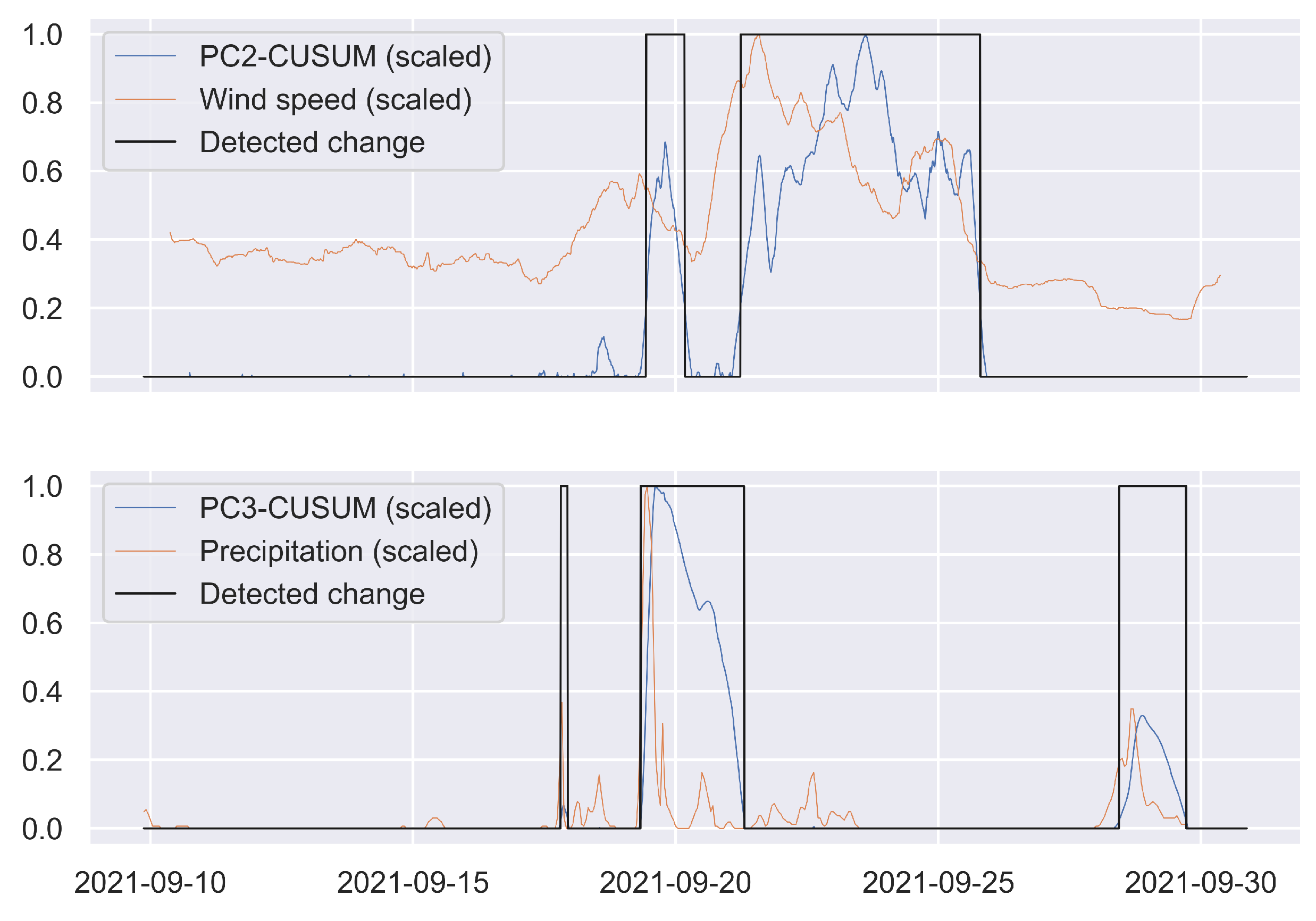
where x t is the current value of the variable (in this case the PC), μ is the mean value of the variable over all time steps, and C is an assigned sensitivity parameter. A change is detected if S t > T , where T is a chosen threshold value. In this case, the chosen values are: C = 1 for both components, T = 5 for PC2, and T = 30 for PC3. The detected changes are shown in Figure 14, along with the scaled cumulative values, wind speed, and precipitation.
Further, in this study, the periods when S t > T , shown as detected change equal to one in Figure 14, are considered representative of the occurrences of significant wind and rain events. The times of occurrence of these events are important, as their effects on the performance of the PV module can come with a time lag, i.e., these effects may be observed after an unspecified period following the event.
For instance, wind can have both direct and delayed effects. It can have an immediate effect on the performance of the module by cooling it in sunny weather, which is a possible reason for the correlations observed in Figure 5 and Figure 12. Notwithstanding, wind and precipitation can occur during the night or on very cloudy days but have a delayed effect on the performance of the module in the following days via reducing the soiling on its surface.

3.3. Wind Speed and Module Temperature

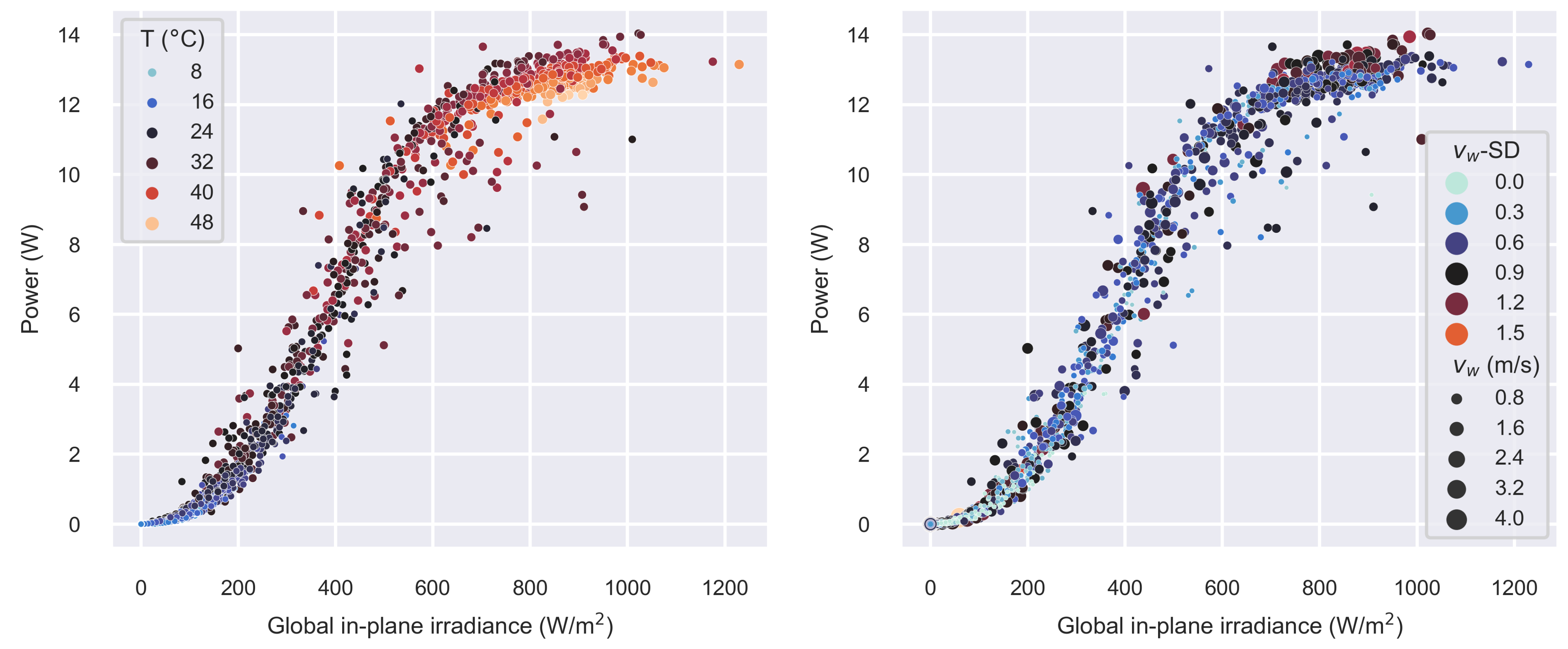
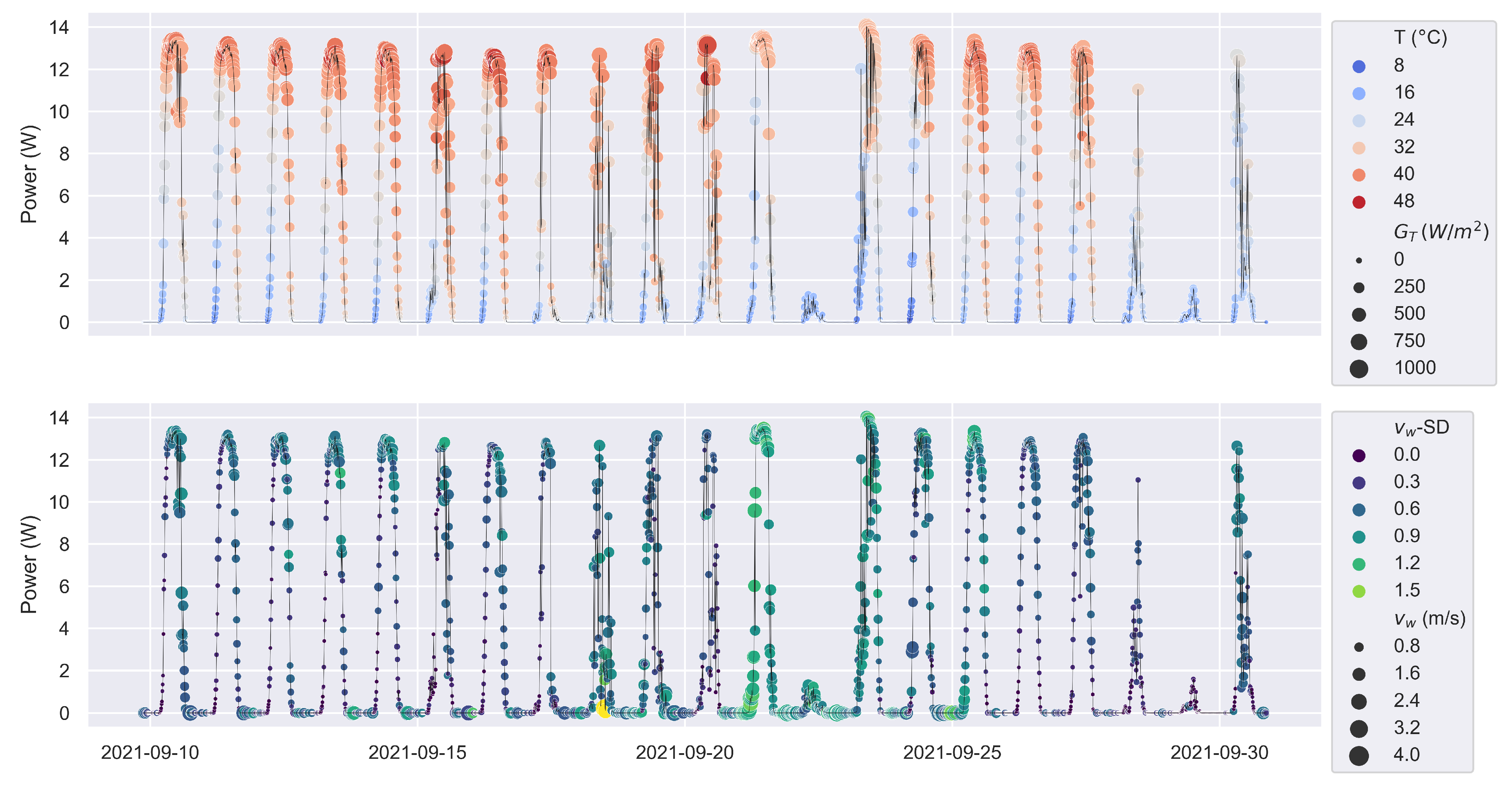
The short-term effects of wind on the performance of the PV module can be observed in Figure 15 and Figure 16. The tendency is evident at irradiance levels above about 600 W m 2 , when the module operates at voltages near to or above V m p and temperature becomes a significant factor for power output (see Figure 2). The scatterplots in Figure 15 show that at higher irradiance, power increases with decreasing temperature, while datapoints associated with lower temperature and higher power are also generally associated with higher wind speed. This is also to a lesser extent visible in Figure 16.
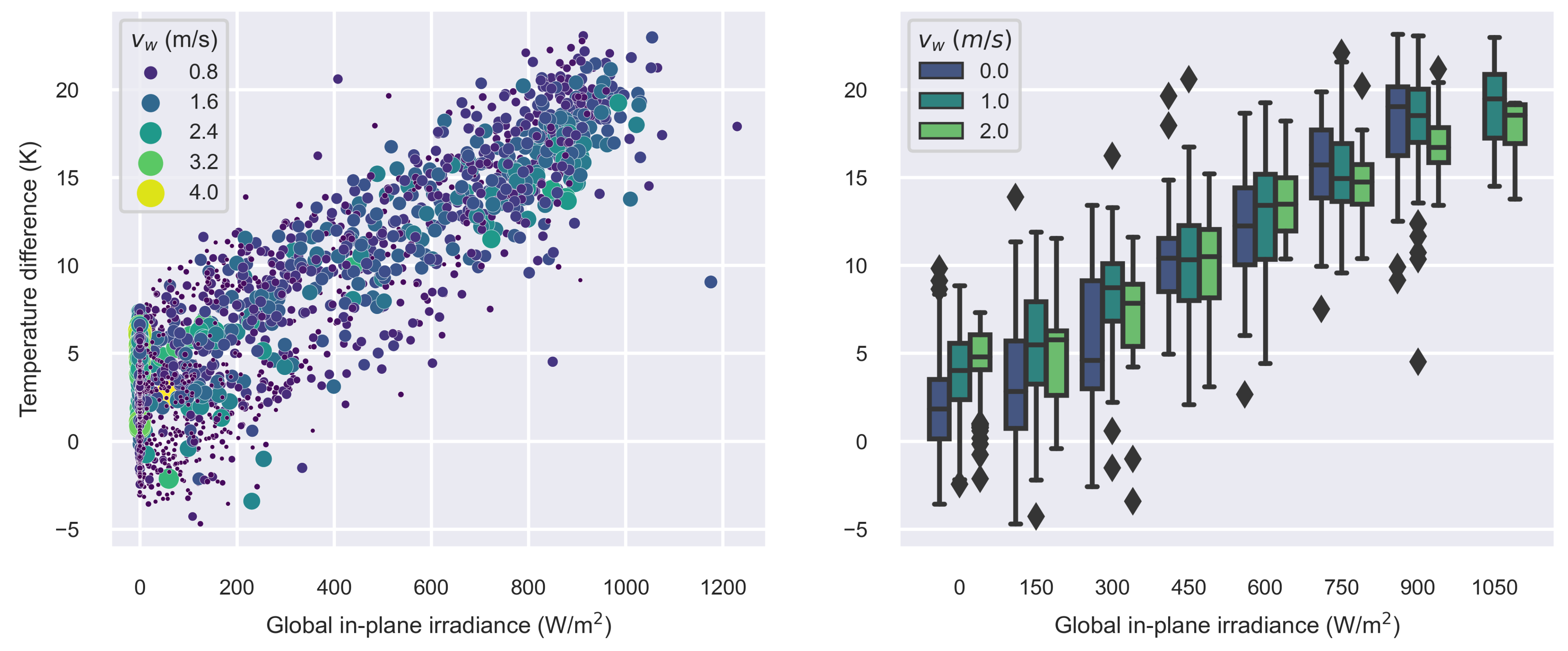
In order to isolate the effect of ambient temperature, the effect of wind speed is also examined on the temperature difference between the module and the ambient air, as shown in Figure 17 and Figure 18. Overall, a clear influence of wind, which can be attributed to its cooling effect on the module’s surface, can be distinguished when the operating point of the module on the I-V curve is near to or to the right of the MPP.

3.4. Seasonal-Trend Decomposition

Soiling is expected to be a cause for deterioration of the PV module’s performance because the test site is in the vicinity of a limestone quarry, which emits significant amounts of dust. However, no measurements or observations regarding the presence of soiling have been taken during the three-week period under investigation.
The primary objective of the study is to assess whether the influence of wind and rainfall on the amount of soiling on the module’s surface can be inferred from the collected weather data. As previously discussed, wind and rainfall can have both positive and negative effects, depending on their intensity and duration. Rain, in particular, is beneficial when it is heavier and prolonged. These potential effects are difficult to observe directly from the original data because of the daily fluctuations and the underlying variabilities of many parameters.
Moreover, the analysis is complicated by the suboptimal performance of the PV module at higher irradiance levels due to the connected constant resistive load. As a result of the latter, the efficiency of the module—defined as the ratio of power output and incident radiation—drops as the irradiance is increased beyond about 600 W m 2 . This can mask some of the soiling-related effects and makes the efficiency unsuitable as a parameter in the analysis.
However, a hypothesis can be made that the significant rain and wind events, identified by the change detection algorithm (see Figure 14), may have produced a detectable influence on the performance of the module. In order to recognize whether such an impact exists, the random noise in the data and the predictable daily variations have to be dealt with in a manner that allows the actual long-term trends in the time series to stand out.
Herein, the technique used for that purpose is seasonal-trend decomposition using locally estimated scatterplot smoothing (LOESS) [83,92]—i.e., STL decomposition—whereby the original data ( Y t ) is decomposed into a sum of three components:
Y t = T t + S t + R t ,
where T t is the trend, S t is the seasonal component, and R t is the remainder.
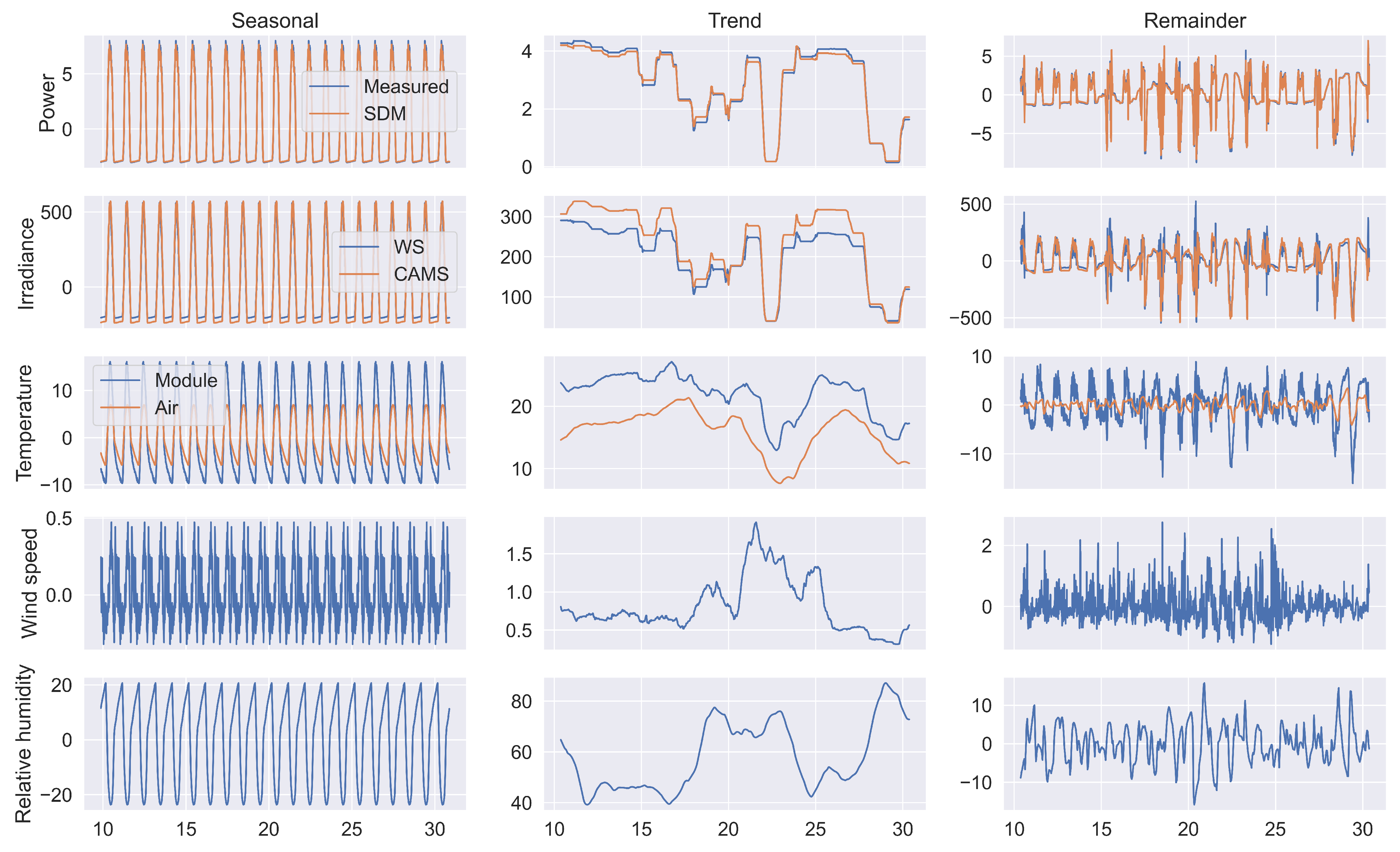
The seasonal component repeats itself after each period (in this case 24 h); the trend captures significant non-periodic variations, while the remainder may be treated as noise depending on the context. The STL decompositions of those original variables from Figure 4 that feature well-defined daily fluctuations are shown in Figure 18. After excluding the seasonal and remainder components, some detectable tendencies emerge. The correlation coefficients of the trend components alone are shown in Figure 19.
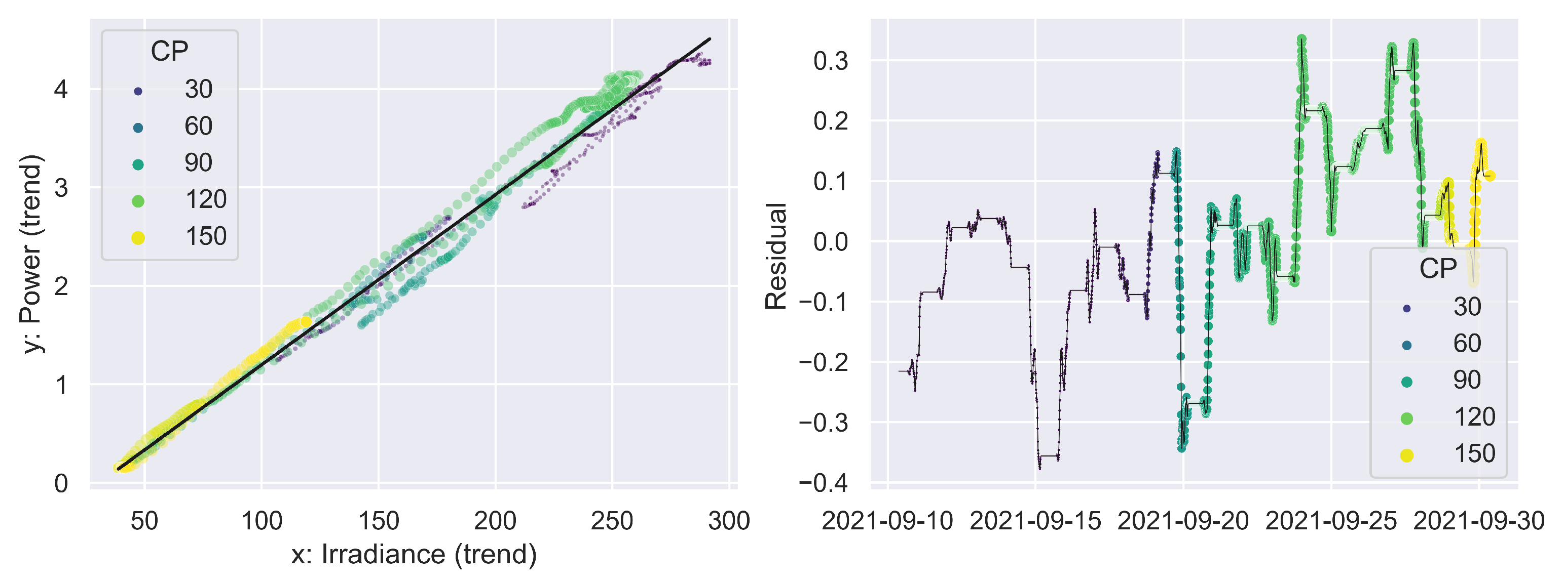
The trend components of module power and irradiance are not only highly correlated, but unlike the original variables, have a strong linear relationship, as shown in Figure 20. Therefore, a linear regression estimator is used to characterize this relationship. (This estimator uses the global in-plane irradiance calculated on the basis of GHI measurements by the pyranometer of the on-site weather station and is hereafter referred to as Model A). In this case, the residuals of the regression model are also interesting, for their temporal distribution can be used as an indicator for changes in module performance. In this context, positive residuals indicate better than average performance, i.e., improvement in the power output trend with respect to the irradiance trend, while negative residuals indicate worse than average performance. The residuals are also plotted in Figure 20 as a time series.
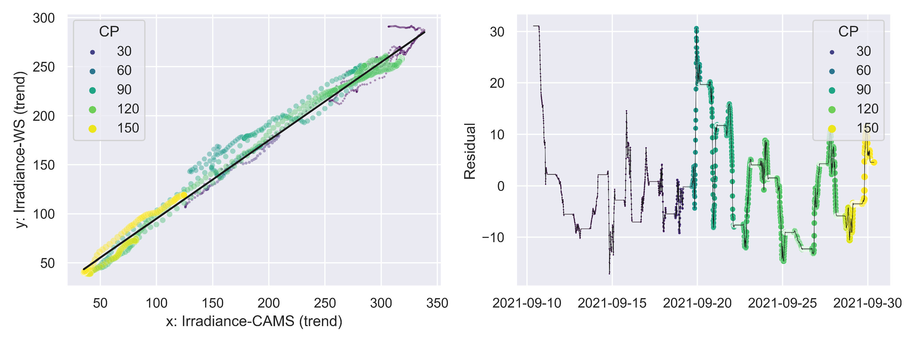
The same procedure is used to compare the two global in-plane irradiance time series, calculated on the basis of GHI data from the two sources, i.e., the on-site pyranometer and the CAMS database (Model B). The results are shown in Figure 21. As shown in Figure 8 and Figure 9, the on-site pyranometer has a tendency to measure lower irradiation than that expected according to the CAMS dataset, which signals the possibility of soiling-related inaccuracies of the former. The residuals of model B are used as a measure of such inaccuracies. The CAMS database relies on models and interpolated data for the GHI values [67,68,69,70]. Although a finely calibrated and well-maintained high-quality pyranometer, situated in the exact location of the PV module, should be able to measure GHI more precisely, in this case the CAMS dataset is used as the benchmark, considering the expected soiling issues.
One of the first observations that can be made is the rapid decline of the residuals of model B after the very first day of measurements. This is a possible indication of swift accumulation of soiling on the pyranometer. Such an indication is also visible in Figure 8, where the significant discrepancies between the two time series appear after the first day. However, this particular finding should be taken with caution—it involves a relatively short interval at the beginning of the three-week period and may be the result of inaccuracies in the data. The drop in the residuals is later followed by a sharp rise around the middle of the period. As shown in Figure 4 and Figure 14, this point in time is around the time of the occurrence of the most significant rainfall.
As a first estimate of the possible effect of rainfall, in Figure 20 and Figure 21, the cumulative precipitation (accounting for the total amount of rain since the beginning of the measurements) is indicated in the size and colour of the datapoints. With this, it becomes obvious that the point of change is exactly during the interval of time with the heaviest rainfall, as indicated by the rapid change of size and colour of the datapoints. A likely conclusion is that the rain has washed off the soiling on the pyranometer’s surface. For some time afterwards, the residuals remain relatively high. However, a few days after the event, they again decline to around their previous level, essentially hinting at a renewed gradual accumulation of soiling. A significant positive change after the occurrence of rain is also observed for the residuals of model A, suggesting that the PV module’s surface has likewise become cleaner, improving the module’s performance.
Considering that the linear regression model for the power trend (model A) is based on the GHI measurements of the weather station, there is a possibility that the improvement of the pyranometer’s conditions initially masks the improvement in the cleanliness of the module’s surface. This might be an explanation for the lagged response of the observed effect on the module’s power output, as seen in Figure 20.
In order to provide an additional point of reference, the procedure for obtaining model A is repeated, but this time using the global in-plane irradiance calculated on the basis of GHI values from the CAMS dataset, thereby obtaining model C. The latter is shown in Figure 22. Similarly to model A, the residuals of model C also exhibit a general positive change after the rainfall, but in this case earlier than those of model A. Indeed, the sharp rise in the residuals of model B after the rainfall is linked to the sharp drop in those of model A, and the latter is thus not observed with model C. The intercept, slope, and coefficient of determination of each of the three models are shown in Table 2.
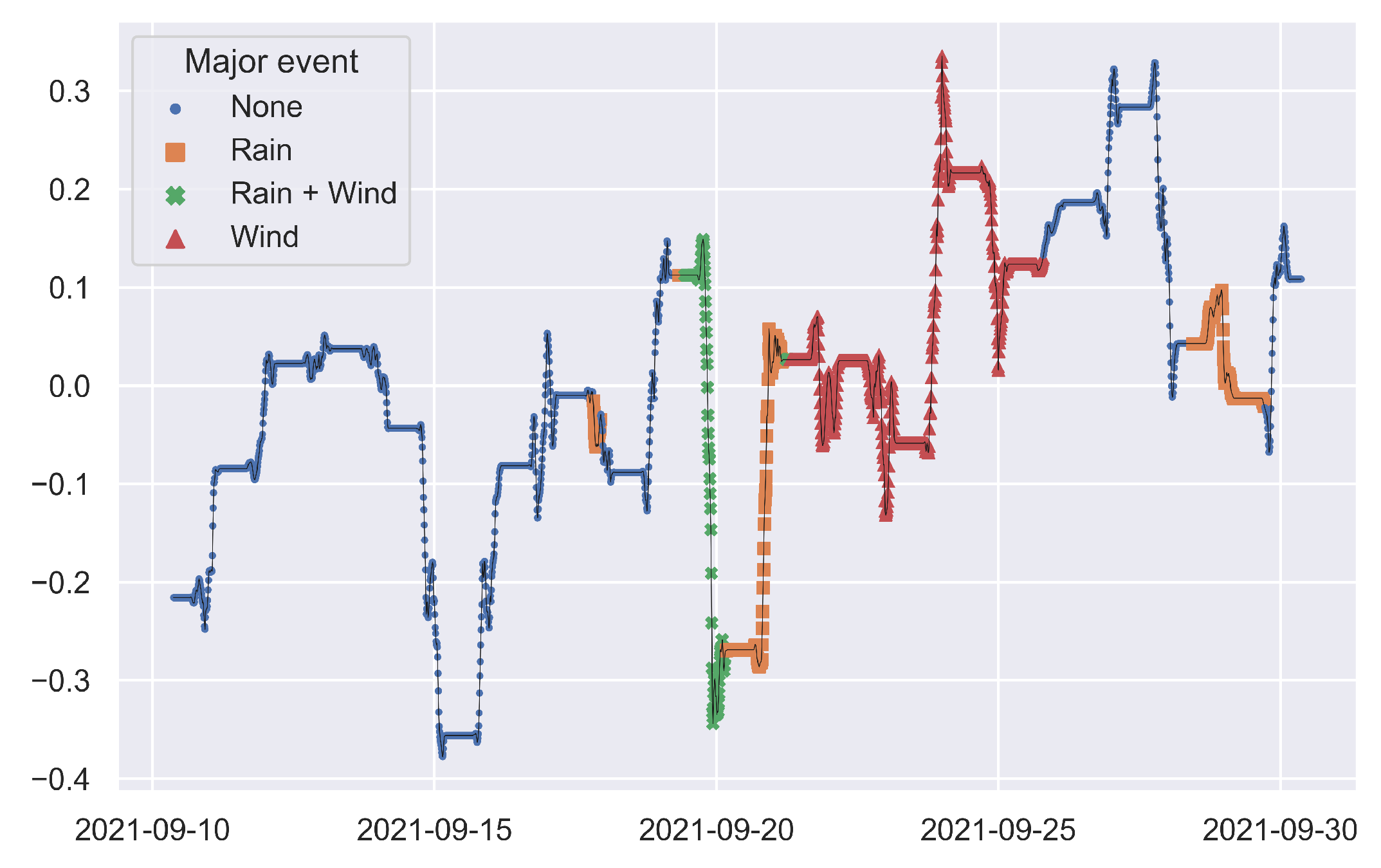
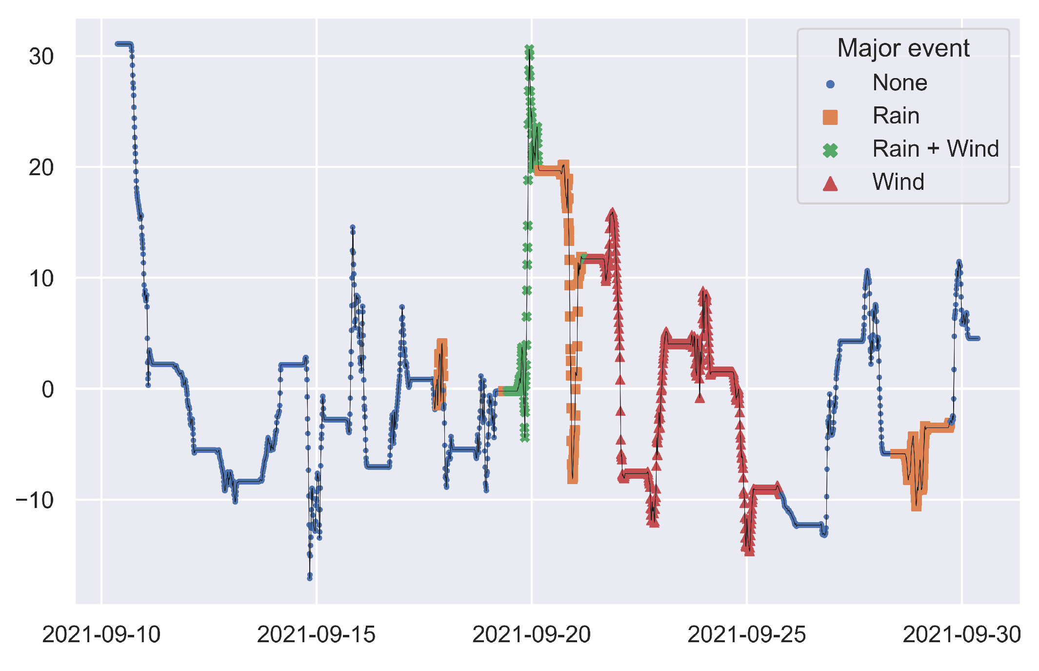
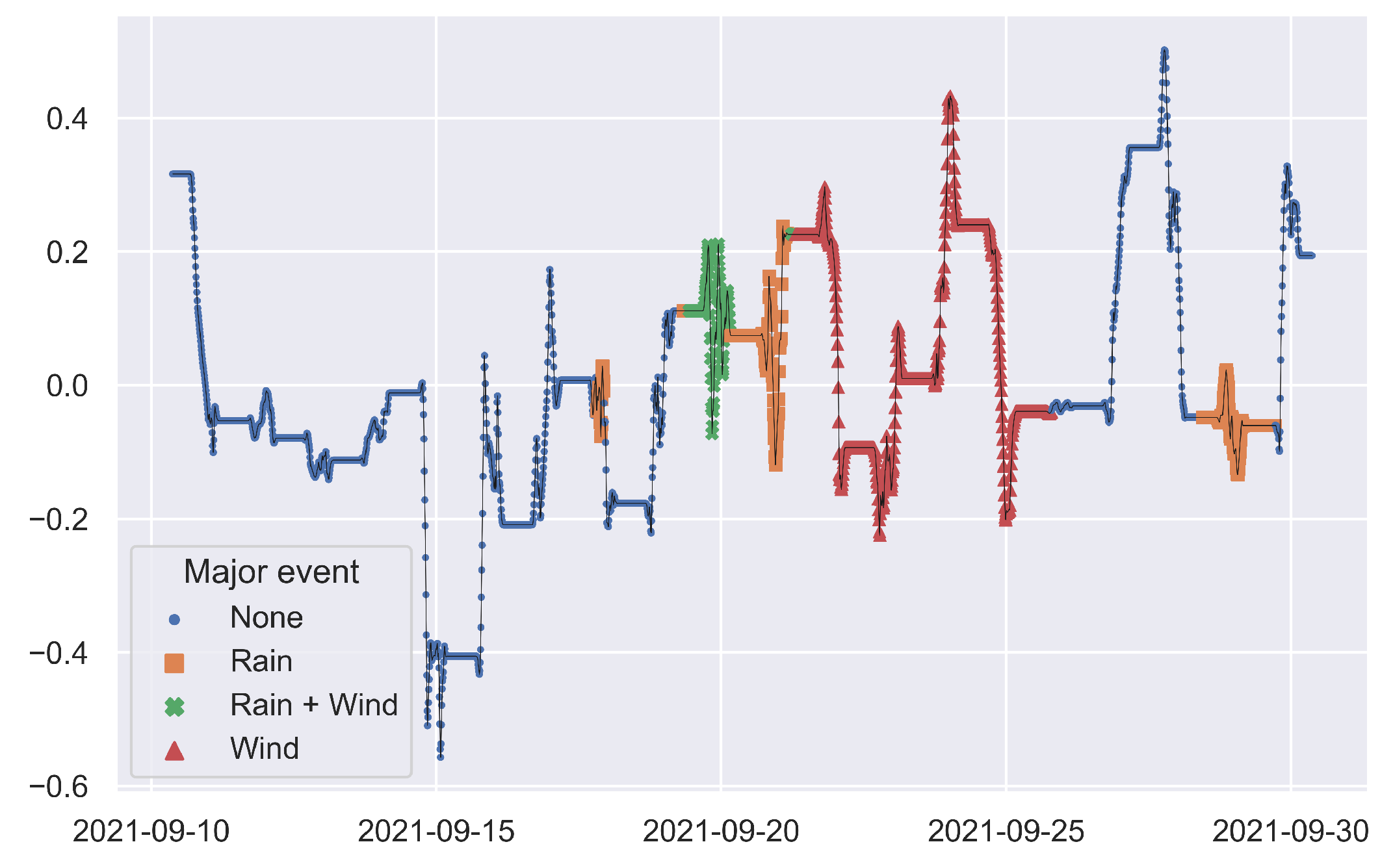
The regression residuals from Figure 20, Figure 21 and Figure 22 are also shown in Figure 23 (for model A), Figure 24 (for model B), and Figure 25 (for model C). However, this time the colouring of the datapoints corresponds to the periods of significant wind and rain events, as identified by the change detection algorithm (see Figure 14).
It becomes clear that the discerned improvement in module performance follows a period characterized by both strong wind and rain, which makes it difficult to distinguish which of the two factors may have contributed more to the cleaning of the module’s surface. In this context, it has to be noted that part of the period characterized by strong wind and/or rainfall is (unsurprisingly) very cloudy, while the module’s power output fluctuates sharply and in some cases is close to zero (see Figure 4). This circumstance could be obscuring the actual moment of significant improvement.
Perhaps—judging from the figures—the most significant episode is the combined rain and wind event around the middle of the period. This is considered hereafter as the threshold event, relative to which the improvement in model performance is evaluated. With this threshold considered, the procedure for obtaining models A and C is repeated, but this time separate linear estimators are used for the datapoints before and after the event, as shown in Figure 26. Regardless of the choice of irradiance data, the slope and more perceivably the intercept of the linear estimator are higher for the datapoints after the threshold event, which confirms the conclusion that the performance of the PV module has improved in the aftermath. The intercept, slope, and coefficient of determination of each model are shown in Table 3.
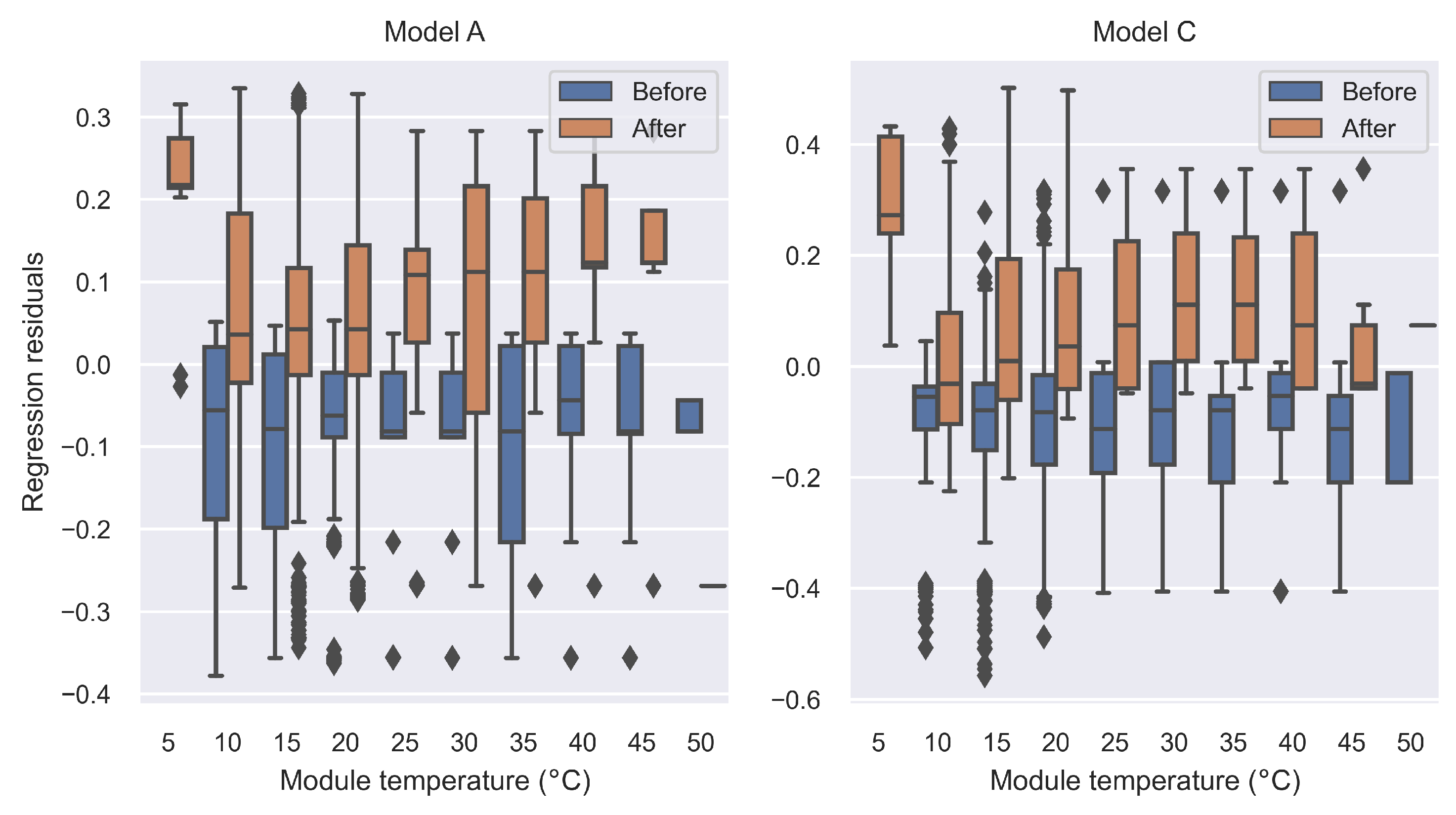
Nevertheless, a hypothesis may arise that the reason behind the perceived improvement in module performance is due to decreasing temperature rather than reduced soiling. This can be part of the explanation, but Figure 27, Figure 28 and Figure 29 indicate an improvement for all temperatures and irradiances. The boxplots in Figure 27 show the residuals of models A and C against module temperature before and after the threshold event. The boxplots demonstrate that in both cases the change after the event is significant for all temperature bins (The last bin is not considered because it includes an insignificant number of datapoints).
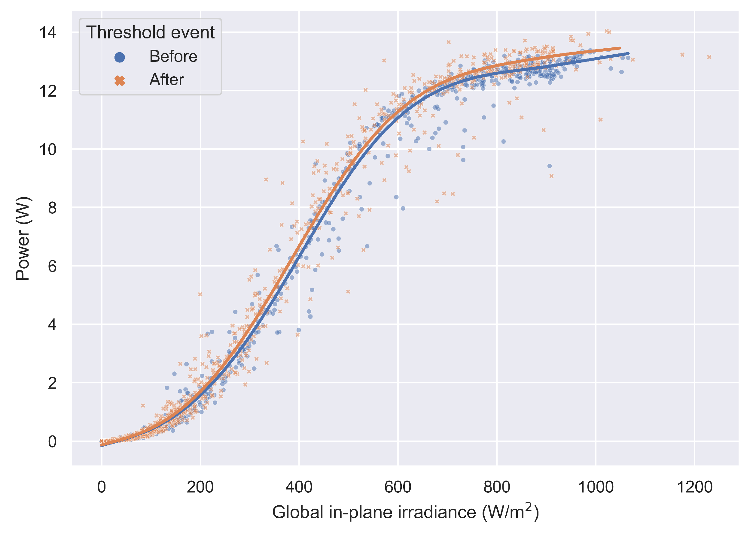
In order to put these results in the context of the original variables, in Figure 28 the power output of the module before and after the threshold event is plotted against the global in-plane irradiance calculated from the measurements of the on-site pyranometer. In general, the datapoints after the event are associated with higher power at the same irradiance level, even though the difference in output is relatively small. To highlight the difference, the two groups of datapoints are fitted by cubic smoothing splines [81] with high values of the regularization parameter. The smoothing splines are fitted after excluding the datapoints with a very high standard deviation of the measured GHI (see Figure 7). The rationale for the exclusion of these datapoints is that they are considered to represent unreliable measurements, associated with large errors arising from time-averaging. These datapoints are nevertheless shown in the scatterplot.
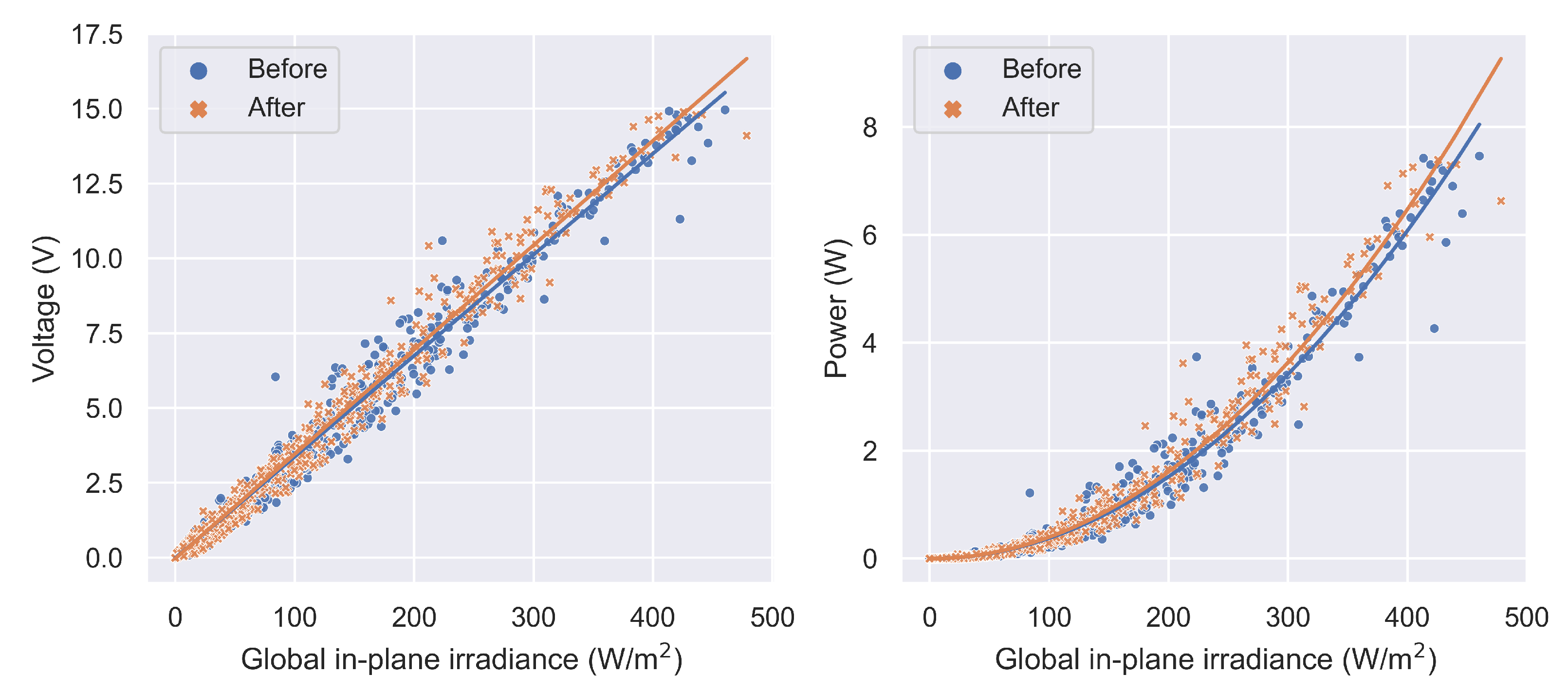
Finally, a comparison is made only for the datapoints where the voltage is below 15 V. For these datapoints, the effect of temperature is insignificant, as the voltage is much lower than that at the MPP (see Figure 1 and Figure 2). Due to the constant resistive load, in this range the voltage increases linearly as a function of irradiance, and thus a linear regression estimator is used to estimate this relationship. The datapoints and the linear estimators for the periods before and after the threshold event are shown in Figure 29 (The datapoints where the standard deviation of GHI is greater than 50 are excluded from the analysis). The intercept, slope, and coefficient of determination of the two models are shown in Table 4. The results in Figure 29 and Table 4 are based on the global in-plane irradiance, as calculated according to the GHI data from the on-site measurements. Similar results are obtained if the GHI values from the CAMS database are used instead, but with much greater variance and thus a lower coefficient of determination.

4. Conclusions

The analysis presented herein reveals that a persistent deterioration of the PV module’s performance as a result of soiling and its subsequent improvement due to a favourable weather event can be detected on the basis of the available data. The analysis does not involve any controlled variables and relies solely on weather data assembled from on-site measurements and other sources, as well as the measured power and temperature of the PV module. Various techniques are employed to isolate the effects of other factors (such as module temperature), so that the observed variations in performance can be attributed to the soiling-related influences.
Based on the analysis, the perceived improvement is likely the result of sufficient rainfall, the effect of which may have been augmented by the stronger than usual winds. Moreover, similar conclusions can be drawn regarding the presence of soiling on the pyranometer’s surface. These findings are consistent with those of many other studies, which have shown that:
  • Soiling is one of the most detrimental factors affecting PV performance, while among the various pollutants, limestone particles are a common cause for concern.
  • In field measurements, the problem with soiling also affects the irradiance sensors, which can obscure the actual magnitude of PV performance deterioration;
  • Rainfall with sufficient intensity can effectively clean soiled surfaces, even if not completely, which makes the issue of soiling much less severe in some climates.
Meanwhile, the study illustrates the difficulties and uncertainties that may arise when dealing with field data and provides some insight into how these issues may be approached to extract meaningful information. While the objective of this study is to identify the soiling-related influences on the basis of limited and uncertain data—which may often be the only such available—much more reliable and quantifiable results can be obtained for research purposes with a proper experimental setup. Nevertheless, it is conceivable that many decisions regarding the planning, operation, and maintenance of PV systems will have to rely on assessments grounded on data suffering from similar issues as encountered here.
In the interest of reproducibility and to give other researchers the ability to use the collected data for their own studies, the dataset from the on-site measurements is made publicly available by the authors (The remaining data are also available from their providers). As discussed herein, the limitations of the included locally measured data should be recognized in order to reduce the risk of misinterpretation. Indeed, the authors recognize the limitations of the presented study and the possibility that a different approach to the analysis may produce diverging outcomes. Therefore, a second part of the study is planned, which would involve a much longer period of measurements, different load charateristics, and additional soiling monitoring (e.g., via a soiling station or soiling image analysis). This further work would allow to test and enhance the presented approach, possibly using the described techniques as building blocks of a more sophisticated algorithm for detecting the impact of soiling from limited data. Such algorithms could be especially useful for soiling detection in smaller, distributed generation PV systems, where the use of more accurate techniques may not be feasible.

Author Contributions

Conceptualization, A.T., B.S., M.V. and M.I.; methodology, B.S. and M.V.; software, B.S.; validation, M.V. and M.I.; formal analysis, B.S.; investigation, A.T. and B.S.; resources, A.T., B.S. and M.V.; data curation, B.S. and M.V.; writing—original draft preparation, B.S.; writing—review and editing, B.S., M.V. and M.I.; visualization, B.S.; supervision, M.I.; project administration, A.T. and M.I.; funding acquisition, A.T. All authors have read and agreed to the published version of the manuscript.

Funding

This study is financed by the European Union—NextGenerationEU, through the National Recovery and Resilience Plan of the Republic of Bulgaria, project № BG-RRP-2.004-0005.

Data Availability Statement

The original data presented in the study are openly available in GitHub at https://github.com/bnstankov/emf-energies24 (accessed on 9 July 2024).

Acknowledgments

Some of the weather data were obtained from the NASA Langley Research Center (LaRC) POWER Project funded through the NASA Earth Science/Applied Science Program. The data were obtained from the POWER Project’s Hourly 2.5.8 version on 1 April 2024. The work also contains modified Copernicus Atmosphere Monitoring Service Information [2021] (Neither the European Commission nor ECMWF is responsible for any use that may be made of the information it contains).

Conflicts of Interest

The authors declare no conflicts of interest. The funders had no role in the design of the study; in the collection, analyses, or interpretation of data; in the writing of the manuscript; or in the decision to publish the results.

Abbreviations

The following abbreviations are used in this manuscript:
CAMSCopernicus Atmosphere Monitoring Service
CUSUMCumulative Sum Method
ECMWFEuropean Centre for Medium-Range Weather Forecasts
GHIGlobal Horizontal Irradiance
HDKRHay-Davies-Klucher-Reindl model
I-VCurrent-Voltage
LOESSLocally Estimated Scatterplot Smoothing
MPPMaximum Power Point
NASANational Aeronautics and Space Administration
PCPrincipal Component
PCAPrincipal Component Analysis
POWERPrediction Of Worldwide Energy Resources
PVPhotovoltaic
SDStandard Deviation
SDMSingle-Diode Model
STLSeasonal-Trend decomposition using LOESS

References

  1. Kruitwagen, L.; Story, K.T.; Friedrich, J.; Byers, L.; Skillman, S.; Hepburn, C. A global inventory of photovoltaic solar energy generating units. Nature 2021, 598, 604–610. [Google Scholar] [CrossRef] [PubMed]
  2. Haegel, N.M.; Verlinden, P.; Victoria, M.; Altermatt, P.; Atwater, H.; Barnes, T.; Breyer, C.; Case, C.; Wolf, S.D.; Deline, C.; et al. Photovoltaics at multi-terawatt scale: Waiting is not an option. Science 2023, 380, 39–42. [Google Scholar] [CrossRef]
  3. Borah, P.; Micheli, L.; Sarmah, N. Analysis of Soiling Loss in Photovoltaic Modules: A Review of the Impact of Atmospheric Parameters, Soil Properties, and Mitigation Approaches. Sustainability 2023, 15, 6669. [Google Scholar] [CrossRef]
  4. Li, X.; Mauzerall, D.L.; Bergin, M.H. Global reduction of solar power generation efficiency due to aerosols and panel soiling. Nat. Sustain. 2020, 3, 720–727. [Google Scholar] [CrossRef]
  5. Jaxa-Rozen, M.; Trutnevyte, E. Sources of uncertainty in long-term global scenarios of solar photovoltaic technology. Nat. Clim. Chang. 2021, 11, 266–273. [Google Scholar] [CrossRef]
  6. Haegel, N.M.; Atwater, H.; Barnes, T.; Breyer, C.; Burrell, A.; Chiang, Y.M.; Wolf, S.D.; Dimmler, B.; Feldman, D.; Glunz, S.; et al. Terawatt-scale photovoltaics: Transform global energy. Science 2019, 364, 836–838. [Google Scholar] [CrossRef] [PubMed]
  7. Shukla, A.K.; Sudhakar, K.; Baredar, P. Recent advancement in BIPV product technologies: A review. Energy Build. 2017, 140, 188–195. [Google Scholar] [CrossRef]
  8. Naderi, M.; Palmer, D.; Smith, M.J.; Ballantyne, E.E.F.; Stone, D.A.; Foster, M.P.; Gladwin, D.T.; Khazali, A.; Al-Wreikat, Y.; Cruden, A.; et al. Techno-Economic Planning of a Fully Renewable Energy-Based Autonomous Microgrid with Both Single and Hybrid Energy Storage Systems. Energies 2024, 17, 788. [Google Scholar] [CrossRef]
  9. Fikiin, K.; Stankov, B. Integration of Renewable Energy in Refrigerated Warehouses. In Handbook of Research on Advances and Applications in Refrigeration Systems and Technologies; IGI Global: Hershey, PA, USA, 2015; pp. 803–853. [Google Scholar] [CrossRef]
  10. Walczewski, M.J.; Wöhrle, H. Prediction of Electricity Generation Using Onshore Wind and Solar Energy in Germany. Energies 2024, 17, 844. [Google Scholar] [CrossRef]
  11. Feron, S.; Cordero, R.R.; Damiani, A.; Jackson, R.B. Climate change extremes and photovoltaic power output. Nat. Sustain. 2021, 4, 270–276. [Google Scholar] [CrossRef]
  12. Van de Ven, D.J.; Capellan-Peréz, I.; Arto, I.; Cazcarro, I.; de Castro, C.; Patel, P.; Gonzalez-Eguino, M. The potential land requirements and related land use change emissions of solar energy. Sci. Rep. 2021, 11, 2907. [Google Scholar] [CrossRef] [PubMed]
  13. Sills, J.; Serrano, D.; Margalida, A.; Pérez-García, J.M.; Juste, J.; Traba, J.; Valera, F.; Carrete, M.; Aihartza, J.; Real, J.; et al. Renewables in Spain threaten biodiversity. Science 2020, 370, 1282–1283. [Google Scholar] [CrossRef]
  14. Ortiz, A.; Negandhi, D.; Mysorekar, S.R.; Nagaraju, S.K.; Kiesecker, J.; Robinson, C.; Bhatia, P.; Khurana, A.; Wang, J.; Oviedo, F.; et al. An Artificial Intelligence Dataset for Solar Energy Locations in India. Sci. Data 2022, 9, 497. [Google Scholar] [CrossRef] [PubMed]
  15. Bao, K.; Thrän, D.; Schröter, B. Land resource allocation between biomass and ground-mounted PV under consideration of the food–water–energy nexus framework at regional scale. Renew. Energy 2023, 203, 323–333. [Google Scholar] [CrossRef]
  16. Rodziewicz, T.; Rajfur, M.; Teneta, J.; Świsłowski, P.; Wacławek, M. Modelling and analysis of the influence of solar spectrum on the efficiency of photovoltaic modules. Energy Rep. 2021, 7, 565–574. [Google Scholar] [CrossRef]
  17. Polman, A.; Knight, M.; Garnett, E.C.; Ehrler, B.; Sinke, W.C. Photovoltaic materials: Present efficiencies and future challenges. Science 2016, 352, aad4424. [Google Scholar] [CrossRef]
  18. Daxini, R.; Wu, Y. Review of methods to account for the solar spectral influence on photovoltaic device performance. Energy 2024, 286, 129461. [Google Scholar] [CrossRef]
  19. Nazir, S.; Ali, A.; Aftab, A.; Muqeet, H.A.; Mirsaeidi, S.; Zhang, J.M. Techno-Economic and Environmental Perspectives of Solar Cell Technologies: A Comprehensive Review. Energies 2023, 16, 4959. [Google Scholar] [CrossRef]
  20. Honsberg, C.; Bowden, S. Photovoltaics Education Website. 2019. Available online: https://www.pveducation.org (accessed on 5 April 2024).
  21. Löper, P.; Pysch, D.; Richter, A.; Hermle, M.; Janz, S.; Zacharias, M.; Glunz, S. Analysis of the Temperature Dependence of the Open-Circuit Voltage. Energy Procedia 2012, 27, 135–142. [Google Scholar] [CrossRef]
  22. Skoplaki, E.; Palyvos, J. On the temperature dependence of photovoltaic module electrical performance: A review of efficiency/power correlations. Sol. Energy 2009, 83, 614–624. [Google Scholar] [CrossRef]
  23. Nižetić, S.; Grubišić- Čabo, F.; Marinić-Kragić, I.; Papadopoulos, A. Experimental and numerical investigation of a backside convective cooling mechanism on photovoltaic panels. Energy 2016, 111, 211–225. [Google Scholar] [CrossRef]
  24. Goverde, H.; Goossens, D.; Govaerts, J.; Catthoor, F.; Baert, K.; Poortmans, J.; Driesen, J. Spatial and temporal analysis of wind effects on PV modules: Consequences for electrical power evaluation. Sol. Energy 2017, 147, 292–299. [Google Scholar] [CrossRef]
  25. Rossa, C. Energy losses in photovoltaic generators due to wind patterns. Commun. Eng. 2023, 2, 66. [Google Scholar] [CrossRef]
  26. Waterworth, D.; Armstrong, A. Southerly winds increase the electricity generated by solar photovoltaic systems. Sol. Energy 2020, 202, 123–135. [Google Scholar] [CrossRef]
  27. Kaplani, E.; Kaplanis, S. Thermal modelling and experimental assessment of the dependence of PV module temperature on wind velocity and direction, module orientation and inclination. Sol. Energy 2014, 107, 443–460. [Google Scholar] [CrossRef]
  28. Ghabuzyan, L.; Pan, K.; Fatahi, A.; Kuo, J.; Baldus-Jeursen, C. Thermal Effects on Photovoltaic Array Performance: Experimentation, Modeling, and Simulation. Appl. Sci. 2021, 11, 1460. [Google Scholar] [CrossRef]
  29. Sharples, S.; Charlesworth, P. Full-scale measurements of wind-induced convective heat transfer from a roof-mounted flat plate solar collector. Sol. Energy 1998, 62, 69–77. [Google Scholar] [CrossRef]
  30. Segbefia, O.K.; Imenes, A.G.; Sætre, T.O. Moisture ingress in photovoltaic modules: A review. Sol. Energy 2021, 224, 889–906. [Google Scholar] [CrossRef]
  31. Mekhilef, S.; Saidur, R.; Kamalisarvestani, M. Effect of dust, humidity and air velocity on efficiency of photovoltaic cells. Renew. Sustain. Energy Rev. 2012, 16, 2920–2925. [Google Scholar] [CrossRef]
  32. Jordan, D.C.; Perry, K.; White, R.; Deline, C. Extreme Weather and PV Performance. IEEE J. Photovolt. 2023, 13, 830–835. [Google Scholar] [CrossRef]
  33. Bošnjaković, M.; Stojkov, M.; Katinić, M.; Lacković, I. Effects of Extreme Weather Conditions on PV Systems. Sustainability 2023, 15, 6044. [Google Scholar] [CrossRef]
  34. Ammari, N.; Mehdi, M.; Alami Merrouni, A.; El Gallassi, H.; Chaabelasri, E.; Ghennioui, A. Experimental study on the impact of soiling on the modules temperature and performance of two different PV technologies under hot arid climate. Heliyon 2022, 8, e11395. [Google Scholar] [CrossRef] [PubMed]
  35. Kaldellis, J.; Fragos, P.; Kapsali, M. Systematic experimental study of the pollution deposition impact on the energy yield of photovoltaic installations. Renew. Energy 2011, 36, 2717–2724. [Google Scholar] [CrossRef]
  36. Kaldellis, J.; Kapsali, M. Simulating the dust effect on the energy performance of photovoltaic generators based on experimental measurements. Energy 2011, 36, 5154–5161. [Google Scholar] [CrossRef]
  37. Mustafa, R.J.; Gomaa, M.R.; Al-Dhaifallah, M.; Rezk, H. Environmental Impacts on the Performance of Solar Photovoltaic Systems. Sustainability 2020, 12, 608. [Google Scholar] [CrossRef]
  38. Nezamisavojbolaghi, M.; Davodian, E.; Bouich, A.; Tlemçani, M.; Mesbahi, O.; Janeiro, F.M. The Impact of Dust Deposition on PV Panels’ Efficiency and Mitigation Solutions: Review Article. Energies 2023, 16, 8022. [Google Scholar] [CrossRef]
  39. Klugmann-Radziemska, E. Degradation of electrical performance of a crystalline photovoltaic module due to dust deposition in northern Poland. Renew. Energy 2015, 78, 418–426. [Google Scholar] [CrossRef]
  40. Maghami, M.R.; Hizam, H.; Gomes, C.; Radzi, M.A.; Rezadad, M.I.; Hajighorbani, S. Power loss due to soiling on solar panel: A review. Renew. Sustain. Energy Rev. 2016, 59, 1307–1316. [Google Scholar] [CrossRef]
  41. Ghazi, S.; Ip, K. The effect of weather conditions on the efficiency of PV panels in the southeast of UK. Renew. Energy 2014, 69, 50–59. [Google Scholar] [CrossRef]
  42. Ilse, K.; Micheli, L.; Figgis, B.W.; Lange, K.; Daßler, D.; Hanifi, H.; Wolfertstetter, F.; Naumann, V.; Hagendorf, C.; Gottschalg, R.; et al. Techno-Economic Assessment of Soiling Losses and Mitigation Strategies for Solar Power Generation. Joule 2019, 3, 2303–2321. [Google Scholar] [CrossRef]
  43. Alkharusi, T.; Huang, G.; Markides, C.N. Characterisation of soiling on glass surfaces and their impact on optical and solar photovoltaic performance. Renew. Energy 2024, 220, 119422. [Google Scholar] [CrossRef]
  44. Sarver, T.; Al-Qaraghuli, A.; Kazmerski, L.L. A comprehensive review of the impact of dust on the use of solar energy: History, investigations, results, literature, and mitigation approaches. Renew. Sustain. Energy Rev. 2013, 22, 698–733. [Google Scholar] [CrossRef]
  45. Appels, R.; Muthirayan, B.; Beerten, A.; Paesen, R.; Driesen, J.; Poortmans, J. The effect of dust deposition on photovoltaic modules. In Proceedings of the 2012 38th IEEE Photovoltaic Specialists Conference, Austin, TX, USA, 3–8 June 2012; pp. 1886–1889. [Google Scholar] [CrossRef]
  46. Zahedi, R.; Ranjbaran, P.; Gharehpetian, G.B.; Mohammadi, F.; Ahmadiahangar, R. Cleaning of Floating Photovoltaic Systems: A Critical Review on Approaches from Technical and Economic Perspectives. Energies 2021, 14, 2018. [Google Scholar] [CrossRef]
  47. Brahma, H.; Pant, S.; Micheli, L.; Smestad, G.P.; Sarmah, N. Effect of Environmental Factors on Photovoltaic Soiling: Experimental and Statistical Analysis. Energies 2023, 16, 45. [Google Scholar] [CrossRef]
  48. Javed, W.; Guo, B.; Figgis, B.; Martin Pomares, L.; Aïssa, B. Multi-year field assessment of seasonal variability of photovoltaic soiling and environmental factors in a desert environment. Sol. Energy 2020, 211, 1392–1402. [Google Scholar] [CrossRef]
  49. Del Pero, C.; Aste, N.; Leonforte, F. The effect of rain on photovoltaic systems. Renew. Energy 2021, 179, 1803–1814. [Google Scholar] [CrossRef]
  50. Picotti, G.; Borghesani, P.; Cholette, M.; Manzolini, G. Soiling of solar collectors—Modelling approaches for airborne dust and its interactions with surfaces. Renew. Sustain. Energy Rev. 2018, 81, 2343–2357. [Google Scholar] [CrossRef]
  51. Amer Dahham, I.; Mohd Zainuri, M.A.A.; Abdullah, A.A.; Fauzan, M.F. Modeling the Effect of Dust and Wind Speed on Solar Panel Performance in Iraq. Energies 2023, 16, 6397. [Google Scholar] [CrossRef]
  52. Goossens, D.; Van Kerschaever, E. Aeolian dust deposition on photovoltaic solar cells: The effects of wind velocity and airborne dust concentration on cell performance. Sol. Energy 1999, 66, 277–289. [Google Scholar] [CrossRef]
  53. Jiang, Y.; Lu, L.; Ferro, A.R.; Ahmadi, G. Analyzing wind cleaning process on the accumulated dust on solar photovoltaic (PV) modules on flat surfaces. Sol. Energy 2018, 159, 1031–1036. [Google Scholar] [CrossRef]
  54. Mani, M.; Pillai, R. Impact of dust on solar photovoltaic (PV) performance: Research status, challenges and recommendations. Renew. Sustain. Energy Rev. 2010, 14, 3124–3131. [Google Scholar] [CrossRef]
  55. Said, S.A.; Walwil, H.M. Fundamental studies on dust fouling effects on PV module performance. Sol. Energy 2014, 107, 328–337. [Google Scholar] [CrossRef]
  56. Figgis, B.; Ennaoui, A.; Ahzi, S.; Rémond, Y. Review of PV soiling particle mechanics in desert environments. Renew. Sustain. Energy Rev. 2017, 76, 872–881. [Google Scholar] [CrossRef]
  57. Ramirez-Vergara, J.; Bosman, L.B.; Wollega, E.; Leon-Salas, W.D. Review of forecasting methods to support photovoltaic predictive maintenance. Clean. Eng. Technol. 2022, 8, 100460. [Google Scholar] [CrossRef]
  58. Araujo Costa Silva, L.; Baca Ruiz, L.G.; Criado-Ramón, D.; Gabriel Bessa, J.; Micheli, L.; del Carmen Pegalajar Jiménez, M. Assessing the impact of soiling on photovoltaic efficiency using supervised learning techniques. Expert Syst. Appl. 2023, 231, 120816. [Google Scholar] [CrossRef]
  59. Bosman, L.B.; Leon-Salas, W.D.; Hutzel, W.; Soto, E.A. PV System Predictive Maintenance: Challenges, Current Approaches, and Opportunities. Energies 2020, 13, 1398. [Google Scholar] [CrossRef]
  60. Bessa, J.G.; Micheli, L.; Almonacid, F.; Fernández, E.F. Monitoring photovoltaic soiling: Assessment, challenges, and perspectives of current and potential strategies. iScience 2021, 24, 102165. [Google Scholar] [CrossRef] [PubMed]
  61. Duffie, J.A.; Beckman, W.A.; Blair, N. Design of Photovoltaic Systems. In Solar Engineering of Thermal Processes, Photovoltaics and Wind; Wiley: Hoboken, NJ, USA, 2020. [Google Scholar] [CrossRef]
  62. Dobos, A.P. An Improved Coefficient Calculator for the California Energy Commission 6 Parameter Photovoltaic Module Model. J. Sol. Energy Eng. 2012, 134, 021011. [Google Scholar] [CrossRef]
  63. Andrews, R.W.; Stein, J.S.; Hansen, C.; Riley, D. Introduction to the open source PV LIB for python Photovoltaic system modelling package. In Proceedings of the 2014 IEEE 40th Photovoltaic Specialist Conference (PVSC), Denver, CO, USA, 8–13 June 2014; pp. 170–174. [Google Scholar] [CrossRef]
  64. Anderson, K.S.; Hansen, C.W.; Holmgren, W.F.; Jensen, A.R.; Mikofski, M.A.; Driesse, A. pvlib python: 2023 project update. J. Open Source Softw. 2023, 8, 5994. [Google Scholar] [CrossRef]
  65. NASA Prediction of Worldwide Energy Resources (POWER). Available online: https://power.larc.nasa.gov (accessed on 1 April 2024).
  66. CAMS Solar Radiation Time-Series. Copernicus Atmosphere Monitoring Service (CAMS) Atmosphere Data Store (ADS). Available online: https://ads.atmosphere.copernicus.eu/cdsapp#!/dataset/cams-solar-radiation-timeseries?tab=overview (accessed on 5 April 2024).
  67. Qu, Z.; Oumbe, A.; Blanc, P.; Espinar, B.; Gesell, G.; Gschwind, B.; Klüser, L.; Lefèvre, M.; Saboret, L.; Schroedter-Homscheidt, M.; et al. Fast radiative transfer parameterisation for assessing the surface solar irradiance: The Heliosat-4 method. Meteorol. Z. 2017, 26, 33–57. [Google Scholar] [CrossRef]
  68. Schroedter-Homscheidt, M.; Azam, F.; Betcke, J.; Hanrieder, N.; Lefèvre, M.; Saboret, L.; Saint-Drenan, Y.M. Surface solar irradiation retrieval from MSG/SEVIRI based on APOLLO Next Generation and HELIOSAT-4 methods. Meteorol. Z. 2022, 31, 455–476. [Google Scholar] [CrossRef]
  69. Gschwind, B.; Wald, L.; Blanc, P.; Lefèvre, M.; Schroedter?Homscheidt, M.; Arola, A. Improving the McClear model estimating the downwelling solar radiation at ground level in cloud?free conditions—McClear-v3. Meteorol. Z. 2019, 28, 147–163. [Google Scholar] [CrossRef]
  70. Lefèvre, M.; Oumbe, A.; Blanc, P.; Espinar, B.; Gschwind, B.; Qu, Z.; Wald, L.; Schroedter-Homscheidt, M.; Hoyer-Klick, C.; Arola, A.; et al. McClear: A new model estimating downwelling solar radiation at ground level in clear-sky conditions. Atmos. Meas. Tech. 2013, 6, 2403–2418. [Google Scholar] [CrossRef]
  71. Erbs, D.; Klein, S.; Duffie, J. Estimation of the diffuse radiation fraction for hourly, daily and monthly-average global radiation. Sol. Energy 1982, 28, 293–302. [Google Scholar] [CrossRef]
  72. Kasten, F.; Young, A.T. Revised optical air mass tables and approximation formula. Appl. Optics 1989, 28, 4735–4738. [Google Scholar] [CrossRef]
  73. Osterwald, C.R.; Adelstein, J.; del Cueto, J.A.; Sekulic, W.; Trudell, D.; McNutt, P.; Hansen, R.; Rummel, S.; Anderberg, A.; Moriarty, T. Resistive loading of photovoltaic modules and arrays for long-term exposure testing. Prog. Photovolt. Res. Appl. 2006, 14, 567–575. [Google Scholar] [CrossRef]
  74. Harris, C.R.; Millman, K.J.; van der Walt, S.J.; Gommers, R.; Virtanen, P.; Cournapeau, D.; Wieser, E.; Taylor, J.; Berg, S.; Smith, N.J.; et al. Array programming with NumPy. Nature 2020, 585, 357–362. [Google Scholar] [CrossRef]
  75. The Pandas Development Team. Pandas-Dev/Pandas: Pandas. 2023. Available online: https://zenodo.org/records/10957263 (accessed on 1 April 2024).
  76. McKinney, W. Data Structures for Statistical Computing in Python. In Proceedings of the 9th Python in Science Conference, Austin, TX, USA, 28 June–3 July 2010; pp. 56–61. [Google Scholar] [CrossRef]
  77. McKinney, W. Python for Data Analysis: Data Wrangling with Pandas, NumPy, and Jupyter; O’Reilly: Sebastopol, CA, USA, 2022. [Google Scholar]
  78. Hunter, J.D. Matplotlib: A 2D graphics environment. Comput. Sci. Eng. 2007, 9, 90–95. [Google Scholar] [CrossRef]
  79. Waskom, M.L. seaborn: Statistical data visualization. J. Open Source Softw. 2021, 6, 3021. [Google Scholar] [CrossRef]
  80. Virtanen, P.; Gommers, R.; Oliphant, T.E.; Haberland, M.; Reddy, T.; Cournapeau, D.; Burovski, E.; Peterson, P.; Weckesser, W.; Bright, J.; et al. SciPy 1.0: Fundamental Algorithms for Scientific Computing in Python. Nat. Methods 2020, 17, 261–272. [Google Scholar] [CrossRef]
  81. Hastie, T.; Tibshirani, R.; Friedman, J. Basis Expansions and Regularization. In The Elements of Statistical Learning: Data Mining, Inference, and Prediction; Springer: New York, NY, USA, 2009; pp. 139–189. [Google Scholar] [CrossRef]
  82. Seabold, S.; Perktold, J. statsmodels: Econometric and statistical modeling with Python. In Proceedings of the 9th Python in Science Conference, Austin, TX, USA, 28 June–3 July 2010; pp. 92–96. [Google Scholar] [CrossRef]
  83. Cleveland, R.B.; Cleveland, W.S.; McRae, J.E.; Terpenning, I. STL: A seasonal-trend decomposition procedure based on Loess. J. Off. Stat. 1990, 6, 3–73. [Google Scholar]
  84. Pedregosa, F.; Varoquaux, G.; Gramfort, A.; Michel, V.; Thirion, B.; Grisel, O.; Blondel, M.; Prettenhofer, P.; Weiss, R.; Dubourg, V.; et al. Scikit-learn: Machine Learning in Python. J. Mach. Learn. Res. 2011, 12, 2825–2830. [Google Scholar]
  85. Greenacre, M.; Groenen, P.J.F.; Hastie, T.; D’Enza, A.I.; Markos, A.; Tuzhilina, E. Principal component analysis. Nat. Rev. Methods Prim. 2022, 2, 100. [Google Scholar] [CrossRef]
  86. Faizi, N.; Alvi, Y. Chapter 6—Correlation. In Biostatistics Manual for Health Research; Faizi, N., Alvi, Y., Eds.; Academic Press: Cambridge, MA, USA, 2023; pp. 109–126. [Google Scholar] [CrossRef]
  87. Orioli, A.; Di Gangi, A. A Criterion for Rating the Usability and Accuracy of the One-Diode Models for Photovoltaic Modules. Energies 2016, 9, 427. [Google Scholar] [CrossRef]
  88. Mihaylov, B.; Betts, T.R.; Pozza, A.; Müllejans, H.; Gottschalg, R. Uncertainty Estimation of Temperature Coefficient Measurements of PV Modules. IEEE J. Photovolt. 2016, 6, 1554–1563. [Google Scholar] [CrossRef]
  89. Feuermann, D.; Zemel, A. Dust-induced degradation of pyranometer sensitivity. Sol. Energy 1993, 50, 483–486. [Google Scholar] [CrossRef]
  90. Geuder, N.; Quaschning, V. Soiling of irradiation sensors and methods for soiling correction. Sol. Energy 2006, 80, 1402–1409. [Google Scholar] [CrossRef]
  91. Ghosh, A. Soiling Losses: A Barrier for India’s Energy Security Dependency from Photovoltaic Power. Challenges 2020, 11, 9. [Google Scholar] [CrossRef]
  92. Cleveland, W.S. Robust Locally Weighted Regression and Smoothing Scatterplots. J. Am. Stat. Assoc. 1979, 74, 829–836. [Google Scholar] [CrossRef]
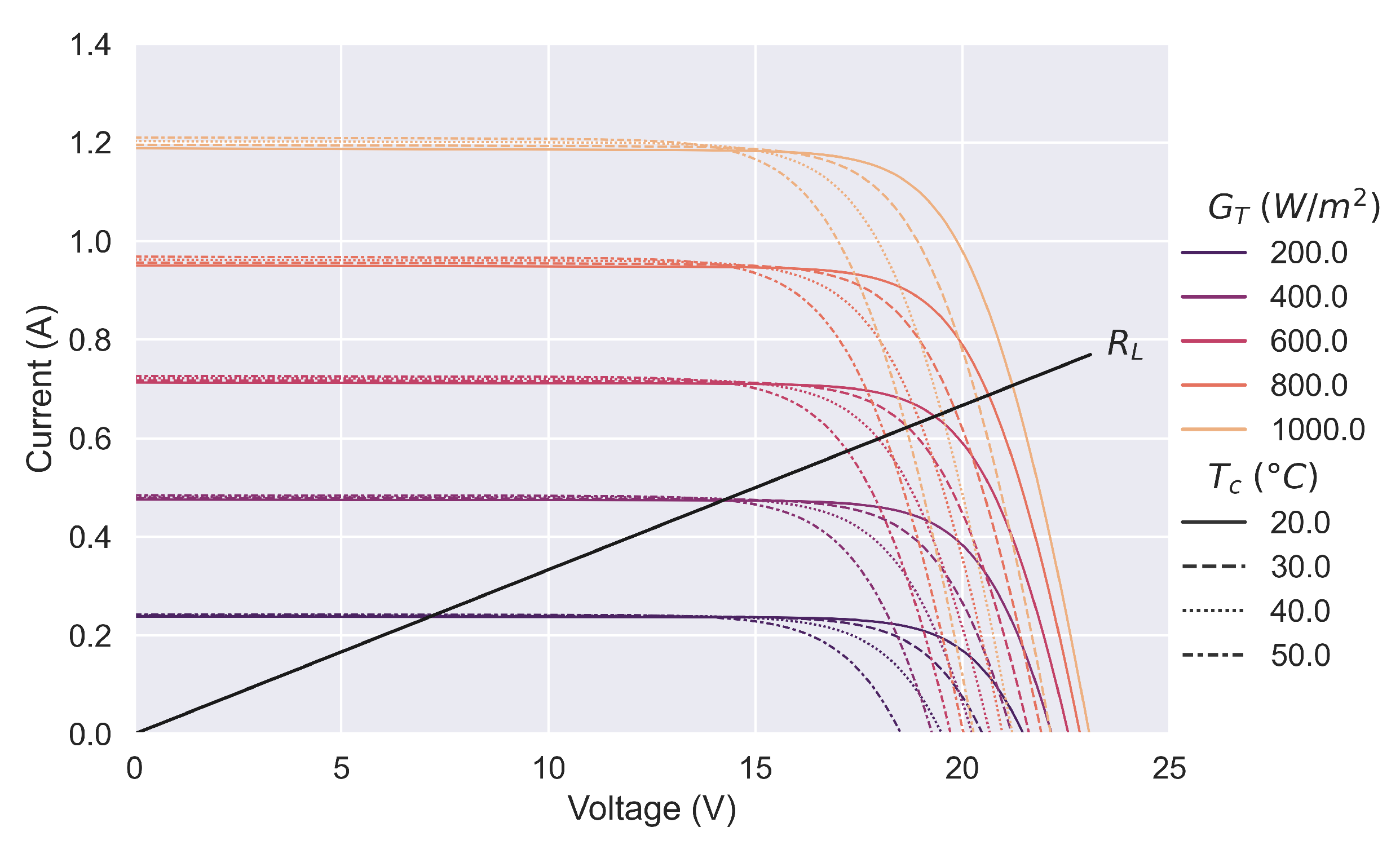
Figure 1. Current-voltage characteristics of the PV module under different operating conditions.
Energies 17 03394 g001
Figure 2. Power-voltage characteristics of the PV module under different operating conditions.
Energies 17 03394 g002
Figure 3. The test site of the study. The module under investigation is the one on the right side of the inclined frame, while the pyranometer and the anemometer are mounted on the neighbouring mast (The PV module on the left side of the inclined frame is not a subject of this study, whereas the other PV modules shown are only used as power sources for the data loggers).
Energies 17 03394 g003
Figure 4. Time series data for the three-week period, including the recorded power of the module and the weather parameters. The temporal resolution is 10 min.
Energies 17 03394 g004
Figure 5. Pearson correlation map of the features in the original time series data.
Energies 17 03394 g005
Figure 6. Measured and modelled power output as functions of global in-plane irradiance.
Energies 17 03394 g006
Figure 7. Measured power output as a function of global in-plane irradiance. The size and colour of the datapoints correspond to the standard deviation of the measured global horizontal irradiance.
Energies 17 03394 g007
Figure 8. Time series comparison between the global horizontal irradiance recorded by the weather station and that obtained from the CAMS database.
Energies 17 03394 g008
Figure 9. Scatterplot comparison between the global horizontal irradiance recorded by the weather station (WS) and that obtained from the CAMS database. The size and colour of the datapoints correspond to the standard deviation (SD) of the measured global horizontal irradiance.
Energies 17 03394 g009
Figure 10. Principal components of the weather data (time series).
Energies 17 03394 g010
Figure 11. Ratio of explained variance by the principal components and Pearson correlation coefficient of each principal component with the power output of the PV module.
Energies 17 03394 g011
Figure 12. Pearson correlation map of the principal components and the originial features.
Energies 17 03394 g012
Figure 13. Scatterplots of the original features and the most significant principal components.
Energies 17 03394 g013
Figure 14. Change detection using the second and third principal components. Detected changes correspond to the occurrence of significant wind or rain events.
Energies 17 03394 g014
Figure 15. Measured power output as a function of global in-plane irradiance. The size and colour of the datapoints correspond to the module’s temperature in the left plot and the mean and standard deviation (SD) of wind speed in the right plot.
Energies 17 03394 g015
Figure 16. Time series of the measured power output. The size and colour of the datapoints correspond to the global in-plane irradiance and module temperature (above) and the mean and standard deviation (SD) of wind speed (below).
Energies 17 03394 g016
Figure 17. Temperature difference between the back surface of the PV module and the ambient air as a function of irradiance. The size and colour of the datapoints correspond to the average wind speed.
Energies 17 03394 g017
Figure 18. STL decomposition of the time series with a 24-h period for the seasonal components.
Energies 17 03394 g018
Figure 19. Pearson correlation map of the trend components from the STL decomposition.
Energies 17 03394 g019
Figure 20. Model A: Linear regression estimator for the relationship between the trend components of measured module power (y) and global in-plane irradiance, calculated from the GHI measurements of the on-site pyranometer (x). The residuals of the model are plotted in time on the right side. The size and colour of the datapoints correspond to cumulative precipitation (mm).
Energies 17 03394 g020
Figure 21. Model B: Linear regression estimator for the relationship between the trend components of global in-plane irradiance, as calculated from the GHI measurements of the on-site pyranometer (y) and the GHI values from the CAMS database (x). The residuals of the model are plotted in time on the right side. The size and colour of the datapoints correspond to cumulative precipitation (mm).
Energies 17 03394 g021
Figure 22. Model C: Linear regression estimator for the relationship between the trend components of measured module power (y) and global in-plane irradiance, calculated according to the GHI values from the CAMS database. The residuals of the model are plotted in time on the right side. The size and colour of the datapoints correspond to cumulative precipitation (mm).
Energies 17 03394 g022
Figure 23. Residuals of model A, plotted in time along with the identified significant weather events.
Energies 17 03394 g023
Figure 24. Residuals of model B, plotted in time along with the identified significant weather events.
Energies 17 03394 g024
Figure 25. Residuals of model C, plotted in time along with the identified significant weather events.
Energies 17 03394 g025
Figure 26. Linear regression estimators for the relationship between the trend components of measured module power (y) and global in-plane irradiance (x), calculated according to the GHI values from the on-site measurements (left) and the CAMS database (right), before and after the threshold event.
Energies 17 03394 g026
Figure 27. Boxplots of the residuals of models A and C, with respect to module temperature (bins) and the periods before and after the threshold event (separate groups within each bin).
Energies 17 03394 g027
Figure 28. Power output of the PV module as a function of global in-plane irradiance before and after the threshold event. The lines shown are cubic smoothing splines.
Energies 17 03394 g028
Figure 29. Voltage (left) and power output (right) of the PV module as a function of global in-plane irradiance, before and after the threshold event, considering only the datapoints where the voltage is below 15 V. The lines shown correspond to the linear regression estimators for the module’s voltage.
Energies 17 03394 g029
Table 1. Temperature coefficients of the PV module.
CoefficientValueUncertainty
Temperature coeffcient of short-circuit current, α s c 0.065 %/K ± 0.01 %/K
Temperature coeffcient of open-circuit voltage, β o c −0.40 %/K ± 0.05 %/K
Temperature coeffcient of maximum power, γ m p −0.5 %/K ± 0.05 %/K
Table 2. Parameters of the linear regression estimators for the module’s voltage.
InterceptSlopeR2
Model A−0.530050.017270.987
Model B15.307170.797170.985
Model C−0.281310.013840.982
Table 3. Parameters of the linear regression estimators for the relationship between the trend components of measured module power (y) and global in-plane irradiance (x), calculated according to the GHI values from the on-site measurements and the CAMS database, before and after the threshold event.
GHI DataThreshold EventInterceptSlopeR2
On-site measurementsBefore−0.491290.014230.972
After−0.305460.014330.990
CAMSBefore−0.635970.017360.985
After−0.574070.017890.991
Table 4. Parameters of the linear regression estimators for the relationship between the module’s voltage (y) and global in-plane irradiance (x).
Threshold EventInterceptSlopeR2
Before−0.012210.033780.987
After−0.033220.034920.988
Disclaimer/Publisher’s Note: The statements, opinions and data contained in all publications are solely those of the individual author(s) and contributor(s) and not of MDPI and/or the editor(s). MDPI and/or the editor(s) disclaim responsibility for any injury to people or property resulting from any ideas, methods, instructions or products referred to in the content.