Abstract
Current artificial intelligence (AI) applications in geothermal exploration are tailored to specific geothermal sites, limiting their transferability and broader applicability. This study aims to develop a globally applicable and transferable geothermal AI model to empower the exploration of geothermal resources. This study presents a methodology for adopting geothermal AI that utilizes known indicators of geothermal areas, including mineral markers, land surface temperature (LST), and faults. The proposed methodology involves a comparative analysis of three distinct geothermal sites—Brady, Desert Peak, and Coso. The research plan includes self-testing to understand the unique characteristics of each site, followed by dependent and independent tests to assess cross-compatibility and model transferability. The results indicate that Desert Peak and Coso geothermal sites are cross-compatible due to their similar geothermal characteristics, allowing the AI model to be transferable between these sites. However, Brady is found to be incompatible with both Desert Peak and Coso. The geothermal AI model developed in this study demonstrates the potential for transferability and applicability to other geothermal sites with similar characteristics, enhancing the efficiency and effectiveness of geothermal resource exploration. This advancement in geothermal AI modeling can significantly contribute to the global expansion of geothermal energy, supporting sustainable energy goals.
1. Introduction
Governments and industry are switching to green energy sources. Many major oil and gas companies have declared their intention to make significant geothermal investments in 2021, considering the volatile price of petroleum resources and helping the global effort to reduce carbon pollution in line with the United Nations Sustainable Development Goals [1]. Geothermal energy is derived from the heat within the Earth’s geological subsurface layers; water and steam are frequently found in geothermal reservoirs at high temperatures. Most geothermal reservoirs are located close to areas of high enthalpies, such as regions of volcanic activity, and are most frequently found close to the tectonic plate boundaries of Earth. Due to a lack of financing and inadequate technology to explore at such depths and high temperatures, geothermal resource development has been moving slowly. Despite the geothermal resource’s remote location and operational challenges, geothermal energy’s long-term sustainability has remained a major attraction for further exploration and exploitation.
Various conventional methods have been used for the exploration of geothermal reservoirs so far. Geophysical methods are fundamental for mapping subsurface structures and identifying potential geothermal reservoirs. Direct geophysical methods provide the most accurate information on geothermal activity, while structural methods reveal geological structures and bodies important for understanding the geothermal system [2]. Geochemical techniques offer valuable insights into the composition of fluids associated with geothermal systems. Geochemical methods characterize reservoir fluids, including sampling and analyzing gas, water, and rock samples. Geochemistry can effectively identify hydraulic fracturing fluids and their sources in the environment, aiding in hydrocarbon resource recovery and wastewater treatment [3]. Another conventional method is seismic tomography, which has become a powerful tool for imaging subsurface structures and understanding reservoir geometry. Seismic tomography is a nondestructive imaging technique that creates cross-sectional pictures of geological targets using the object’s response to an external source’s nondestructive, probing energy [4].
Geothermal exploration often involves a multidisciplinary approach, combining geophysics, geochemistry, seismic surveys, and drilling technologies. Traditional exploration methods like seismic surveys may have limitations in providing high-resolution images of subsurface structures. Crosswell seismic imaging technology provides high-resolution images of reservoir structure and properties, enabling optimized reservoir development programs at a reduced cost [5]. However, low-resolution data can hinder accurate reservoir characterization, potentially leading to suboptimal well placement and reduced overall project efficiency. Traditional geothermal exploration methods, particularly drilling, can be expensive, and the uncertainty associated with resource estimation may contribute to financial risks for project developers [6]. Improving exploration techniques to enhance accuracy can mitigate such financial risks. Geothermal resources are often found in remote or challenging terrains. Conventional exploration methods may face logistical challenges, leading to increased costs and difficulties in reaching and exploring potential geothermal sites. While conventional geothermal exploration methods have been instrumental in developing the geothermal industry, they are not without drawbacks. Addressing these limitations through technological advancements and improved exploration strategies is crucial for enhancing the sustainability and efficiency of geothermal energy development.
Remote sensing (RS) technologies have proven invaluable in exploring and characterizing geothermal areas, providing a non-invasive and comprehensive approach. Researchers used satellite imagery, hyperspectral images [7], thermal infrared sensors [8,9], synthetic aperture radar (SAR) images [10], and other RS tools to detect surface manifestations of geothermal systems. Infrared RS enables the monitoring of thermal anomalies on the Earth’s surface. [11] discuss the application of thermal infrared sensors in detecting temperature variations related to geothermal activity, allowing for the identification of heat flow patterns and anomalies [12] and identifying altered rocks [13] and potential reservoir locations [14].
RS facilitates regional-scale resource assessment by providing synoptic views of large areas. The satellite-based data for regional exploration allow for the rapid identification and evaluation of geothermal prospects over extensive terrains [15,16,17]. Combining RS data with geophysical information enhances the overall understanding of subsurface structures [18]. It discusses integrating satellite imagery with geophysical data, illustrating how these complementary datasets can improve the accuracy of geological and geothermal resource mapping. RS time-series analysis allows for continuous monitoring of geothermal areas, helping to detect changes over time [19], especially monitoring landscape changes and ecosystem health [20].
AI exploiting big data has become a powerful tool in geothermal exploration, offering advanced resource identification, characterization, and monitoring. AI algorithms, particularly those based on machine learning (ML), excel in identifying subtle surface manifestations [21] indicative of geothermal activity. By analyzing multimodal RS images, AI can enhance the detection of features such as hot springs, altered surface minerals, and fumaroles [21]. When coupled with AI algorithms, satellite thermal infrared imagery enables the automated identification of thermal anomalies associated with potential geothermal resources. ML models combined with multispectral and hyperspectral satellite data can rapidly identify geothermal prospects over broad terrains [13]. Deep learning techniques, such as convolutional neural networks (CNNs), enable effective feature extraction from high-resolution satellite images. The application of CNNs for automatically interpreting geophysical features in satellite imagery aids in identifying subsurface structures [21]. AI algorithms applied to time-series satellite imagery enable real-time monitoring and change detection in geothermal areas. These tools can detect variations in land surface temperatures, faults, salt boundaries, subsurface activity, and other environmental changes, providing valuable insights for ongoing exploration and development [21,22].
Integrating AI with satellite images revolutionizes geothermal exploration by enhancing surface manifestation detection, enabling automated thermal anomaly identification, and supporting large-scale resource assessment. As AI and satellite technology continue to advance, their synergistic application holds great potential for the efficient and accurate exploration of geothermal resources. RS, Geographic Information Systems (GIS), and some auxiliary data may help extract the geothermal field accurately by developing AI algorithms.
AI enhances the efficiency and efficacy of geothermal energy systems through predictive maintenance, optimizing drilling processes, and managing energy distribution. Attempts have been made to employ deep learning techniques to predict the potential of geothermal energy [21,23,24,25]. Geothermal energy can also be utilized by ML techniques [26,27].
In recent studies, a thorough analysis of geothermal indicators, namely fault density, mineral markers, and LST, has been presented, and an AI model called geothermal AI was introduced [21]. The model was developed using data from existing Brady and Desert Peak geothermal sites in Nevada, USA. Nevertheless, these two geothermal sites were located near each other and had comparable geological features, primarily in sedimentary lithologies. Because geothermal sites possess diverse geological characteristics, enhancing the existing AI models is imperative to provide accurate assessments of geothermal resources.
Using data from three active geothermal sites—Brady, Desert Peak, and Coso—we created seven distinct AI models for this study, and we evaluated how well they predicted the surface footprint of the available resources. Coso geothermal site is significantly bigger than the other two. Unlike the satellite datasets used for Brady and Desert Peak, it has different geothermal indicator datasets collected and validated by field studies. Moreover, the datasets for geothermal indicators for the three sites are curated using ML algorithms to reveal the pattern of indicators. In this way, we presented a robust, applicable framework to analyze geothermal indicators in a given geothermal site. We fed inputs from the three sites into the seven AI models and evaluated the accuracy of each model. The results of each model improve our comprehension of AI’s ability to anticipate the performance of geothermal resource assessment and provide insights for decision-making in comparable geological situations.
2. Proposed Methodology and Implementation
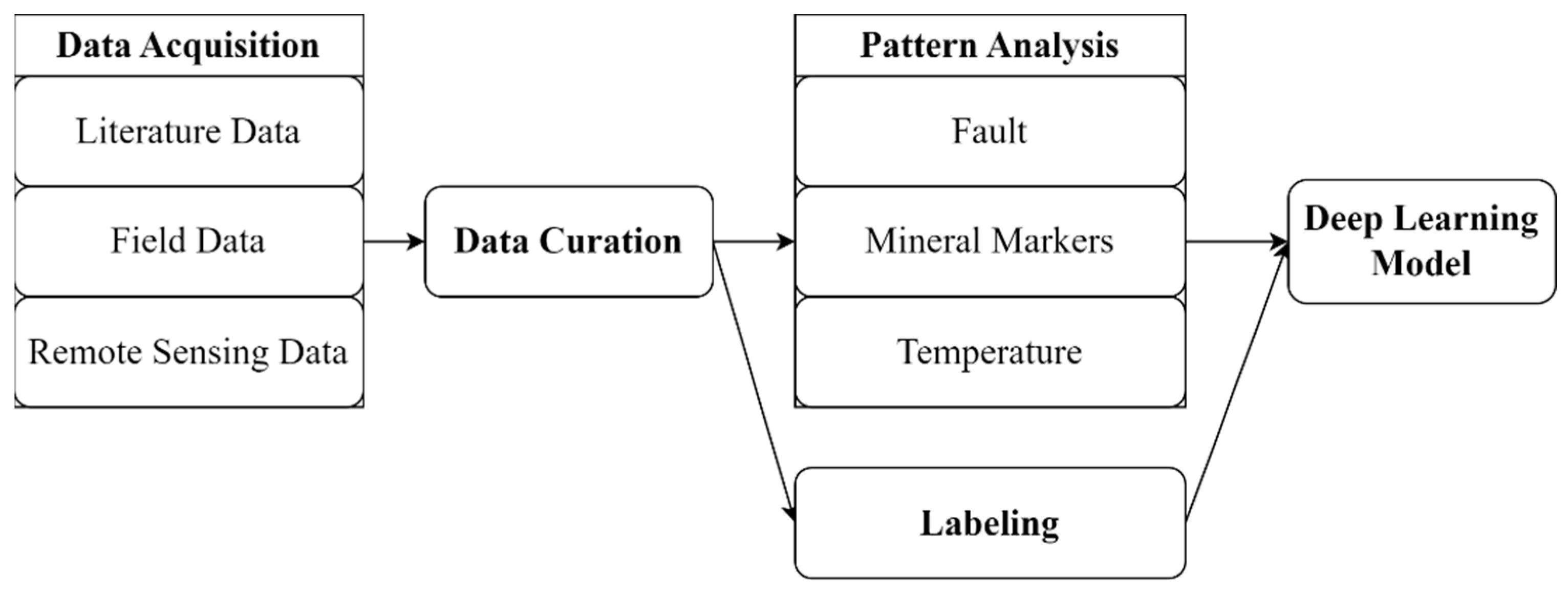
The proposed methodology consists of four phases, as shown in Figure 1. The first phase in developing an AI system for geothermal exploration is data acquisition, which consists of the acquisition of literature data, field data, and RS data. Acquired data needs to be curated at the data curation phase. This step ensures the quality, usability, and accessibility of the data by organizing, cleaning, integrating, and standardizing the data. Pattern analysis, which comprises both temporal and spatial analyses of geothermal indicators, namely faults, mineral markers, and temperature, using ML, is the third step of the system. Labeling provides a way of determining classes of supervised learning, where geothermal and non-geothermal pixels are identified to train the AI algorithm. The deep learning model improves learning by extracting patterns from each geothermal indicator dataset. The following subsections explain each phase in detail.
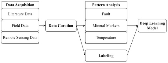
Figure 1.
Research methodology.
2.1. Data Acquisition
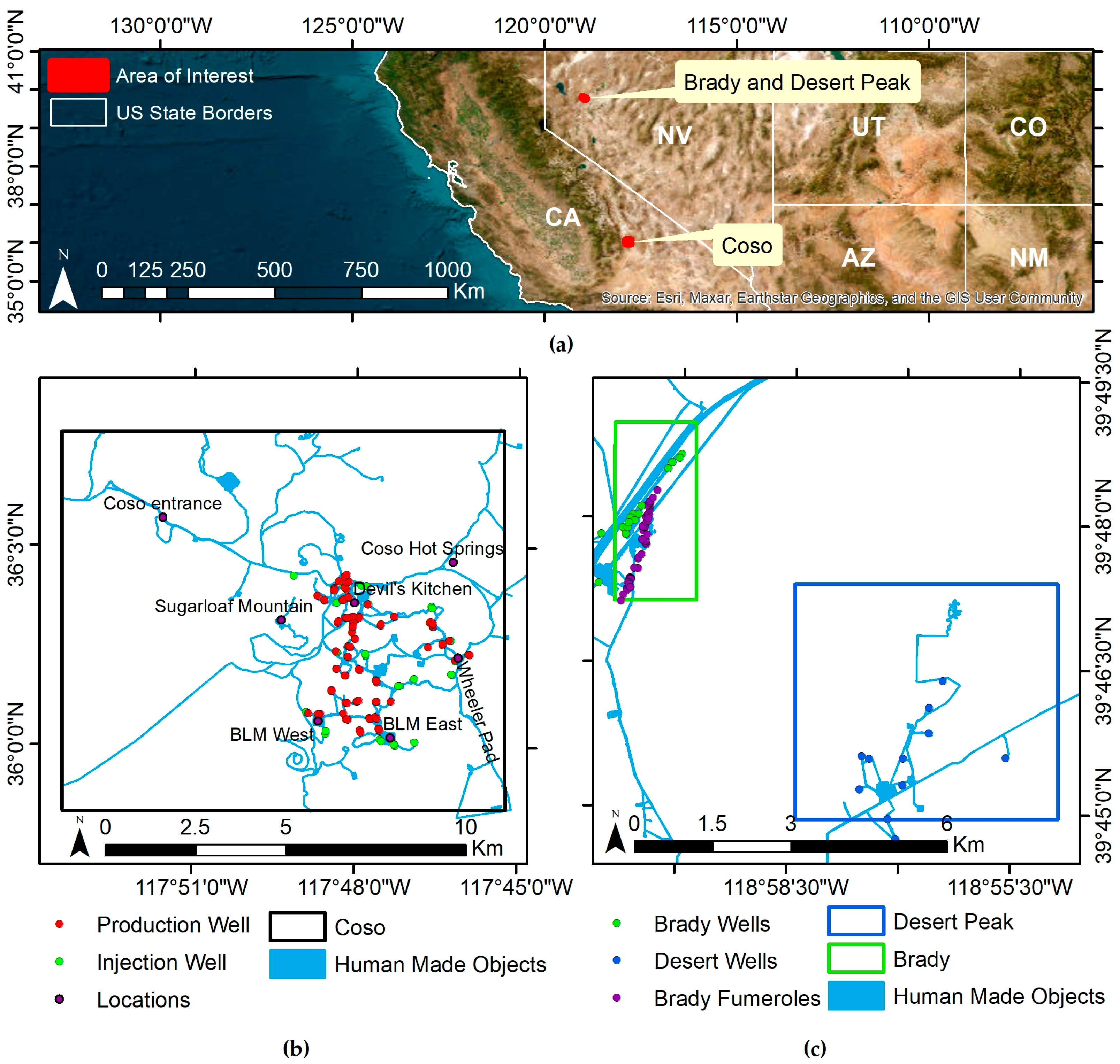
The Brady geothermal field, Desert Peak geothermal field, and Coso geothermal field (CGF) are the three geothermal areas in this study. Brady has surface geothermal features, including active fumaroles, silica sinter, silicified sediments, and warm ground [28,29,30,31,32]. On the other hand, Desert Peak is a blind system with no surface geothermal manifestations [9]. CGF lies in a Pliocene–Pleistocene volcanic field [33] and exhibits surface manifestations like Brady.
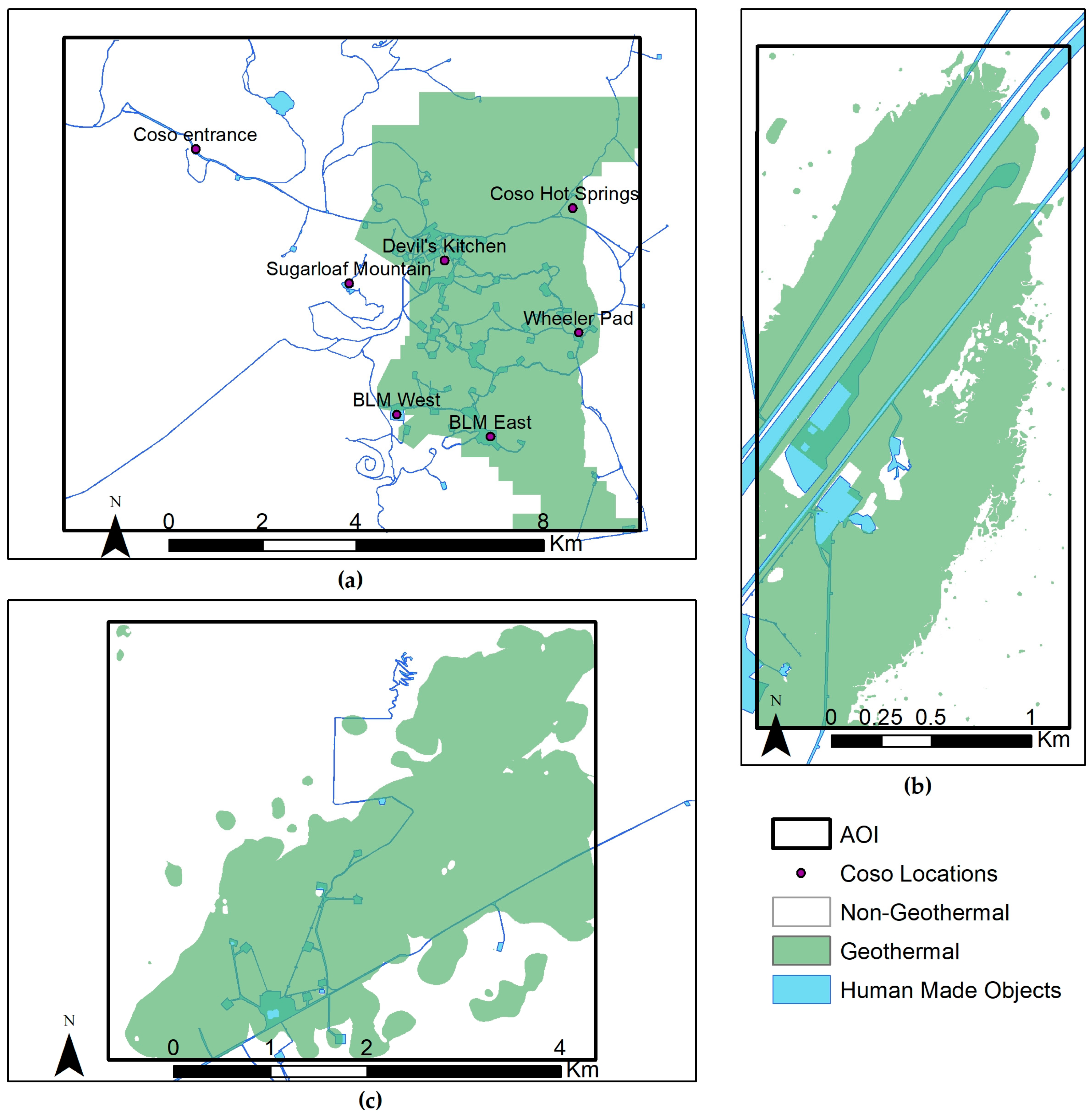
The Northwest Basin and Range Geothermal Region of Nevada includes the Brady Hot Springs Geothermal region (39.79° N, 119.02° W) northeast of Fernley, Nevada. Desert Peak (39.75° N, 118.95° W) is located southeast of the Brady geothermal site, as shown in Figure 2c.
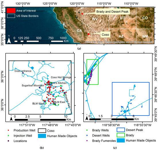
Figure 2.
Map of study areas: (a) General overview map of Brady, Coso, and Desert Peak geothermal fields; (b) Detailed map of Coso geothermal field; (c) Detailed map of Brady and Desert Peak geothermal fields.
Desert Peak and Brady have fault density maps, fusion maps of mineral markers, and LST maps created by fixed k-means clustering methods as inputs. Furthermore, they have ground truth maps created based on deformation in the form of subsidence and uplift. Brady and Desert Peak data have been acquired by RS and Open Energy Information (OpenEI) [34,35]. This study examined the data acquisition, curation, pattern analysis, and labeling steps for CGF since Coso contains distinct data compared to Brady and Desert Peak.
CGF is located in eastern California’s Inyo County, home to one of the country’s biggest geothermal power plants with a maximum capacity of over 270 megawatts (MW). Numerous studies and investigations have been conducted in this field, and OpenEI and its Geothermal Data Repository provide extensive data [36]. Figure 2b also indicates the location of CGF.
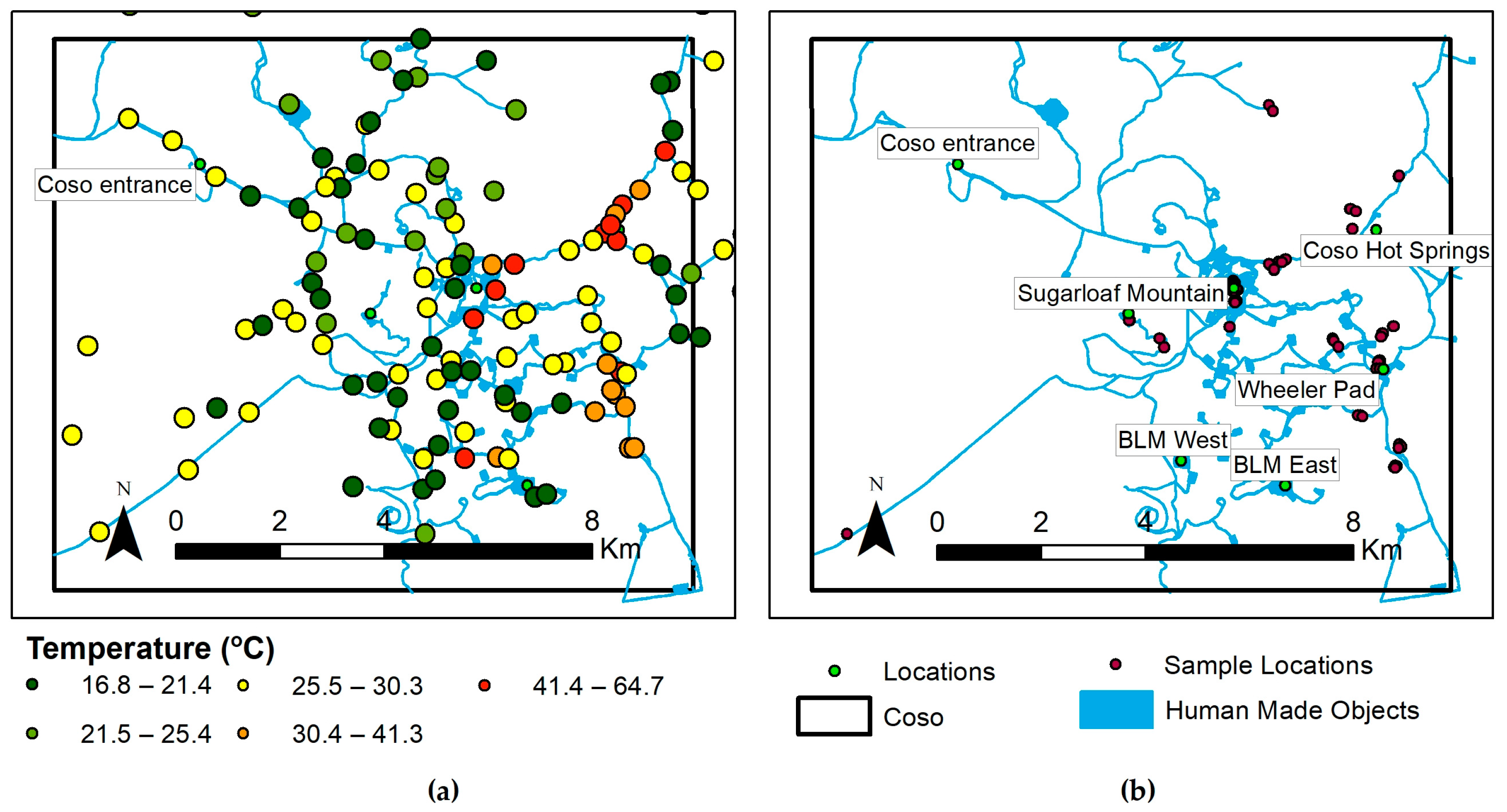
Temperature surveys on CGF have been conducted in previous studies [37,38]. 2 m probe temperature data with 133 points ranging across CGF have been acquired from these studies. The 2 m probe temperature data locations are shown in Figure 3a. Geological studies of the CGF have been ongoing since 1978, with seminal research conducted by [39,40]. Since then, extensive research has been published on the region’s surface geological characteristics and fault systems [41,42,43,44,45]. These studies serve as the sources for the fault data utilized in this study.

Figure 3.
Field data locations: (a) 2 m temperature probe locations; (b) Rock sample locations.
In 2022, the research team completed an extensive CGF study. Ninety-seven geological samples were methodically gathered from several sites in the CGF, including notable geothermal anomaly zones like Devil’s Kitchen, Nicol Pad, and Wheeler Pad (Figure 3b). Additionally, we acquired the reservoir model created for CGF for operation purposes by Coso Operating Company, Little Lake, CA, USA.
RS data can analyze the surface manifestations of geothermal sites. From 2018 to 2022, we acquired 416 LANDSAT 8 Level-2 Provisional Surface Temperature product satellite images covering the CGF. Multispectral images received from the Advanced Spaceborne Thermal and Reflection Radiometer (ASTER) satellite are also used for mineral markers. The data we gathered for CGF came from various sources listed in Table 1.

Table 1.
Data sources of Coso geothermal field for the considered geothermal indicators.
2.2. Data Curation
This step is mainly composed of preprocessing the data, which includes resampling, border matching, and coordinate reference matching. Resampling is the process of changing the resolution of a raster dataset. A 3 × 3 m pixel resolution is used for Coso data to align with the Brady and Desert Peak data. Resolution and border matching are necessary when data are acquired from separate sources so that the geolocations of corresponding pixels of raster data coincide. Coordinate reference matching of all data is also recommended when working in a GIS environment.
2.2.1. Temperature Data Curation
We downloaded 416 images from LANDSAT 8 Level-2 Provisional Surface Temperature images. As shown in Table 2, we applied thresholding to remove the low-quality images for further analysis. LST images from five years (2018–2022) were filtered according to uncertainty values. First, we removed images with high uncertainty. We have set the uncertainty limit to 5 °C. Thus, if any pixel of an image has uncertainty more than the limit value, we removed the entire image from our dataset. Then, the remaining images were filtered out according to pixel quality values. The images were selected such that more than or equal to 70% of the image should have clear pixels, i.e., no snow, no ice, no water, no cloud, and less than 5% of the image should have high-confidence cloud. Finally, we had 85 images available for analysis.

Table 2.
Thresholds applied to LANDSAT images.
Selected images were used for k-means clustering and self-organizing maps (SOM) algorithms to obtain the LST pattern. We also used kriging to interpolate 2 m temperature probe data to obtain a ground-based LST pattern.
2.2.2. Fault Data Curation
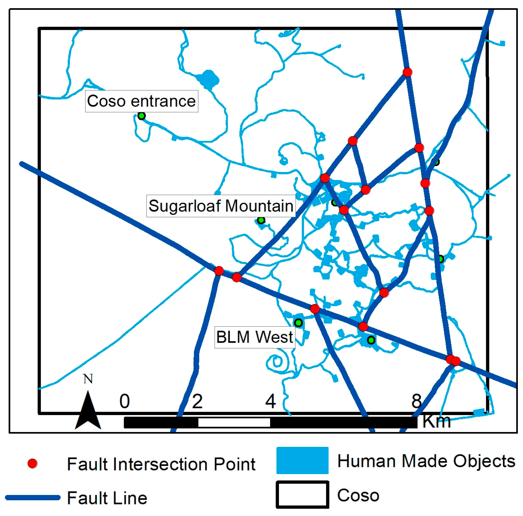
All faults were compiled from various sources, and a preliminary fault map was created in this study. This map shows the potential recurrence of the same faults. Thus, an elimination method was applied together with the experts of the Navy Geothermal Program Office (GPO). This ended up with 14 faults and three underground blind faults. The resulting fault map was based on Duffield, Bacon, and Whitmarsh’s preliminary mineral mapping study and geological maps [46,47]. In addition, we have determined fault line intersection points useful in pattern analysis. The surface fault lines and fault line intersection points in CGF are shown in Figure 4.
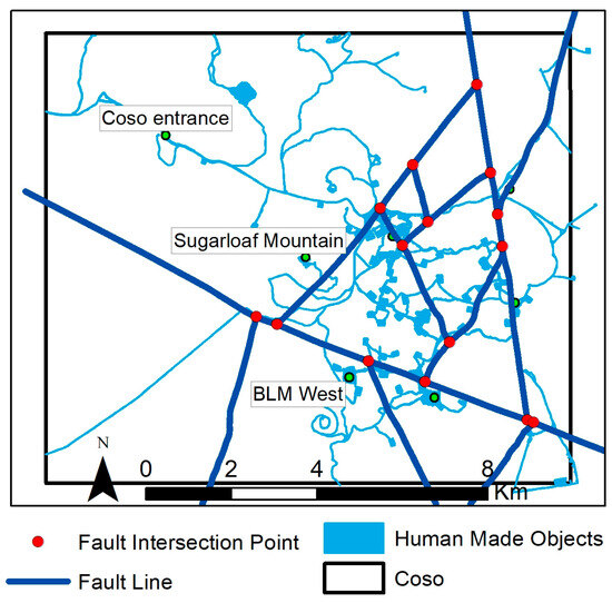
Figure 4.
Fault map of Coso geothermal field [39,40,41,42,43,44,45,46,47].
2.2.3. Alteration Mineral Data Curation
The rock samples obtained from the CGF were pivotal in establishing the dataset for the field visit. By analyzing 97 samples acquired from diverse locales within CGF, the study facilitated the generation of verifiable data and an exclusive spectral library tailored to the CGF. These samples underwent spectral analysis employing an ASD FieldSpec 4 spectroradiometer, and collecting spectral data within controlled parameters reduced variables such as noise or atmospheric errors. In addition to the initial field assessment of the samples’ physical characteristics, laboratory analyses were conducted to ascertain their potential mineral composition. SEM-based automated mineralogy was applied to selected samples to investigate alteration mineralogy, while portable X-ray fluorescence (pXRF) was deployed on most samples to procure supplementary data.
Furthermore, satellite data complemented the field-derived information through target detection analysis. ASTER satellite images were acquired for this purpose, encompassing both VNIR (visible and near-infrared, spanning 400 to 1000 nm) and SWIR (Short-Wavelength Infrared, ranging from 1000 to 2500 nm) spectra. The obtained ASTER dataset in this study comprised Level 1 Precision Terrain Corrected Registered At-Sensor Radiance (AST_L1T) data generated via a singular resampling process of the corresponding ASTER L1A (AST_L1A) product.
2.2.4. Reservoir Model Data Curation
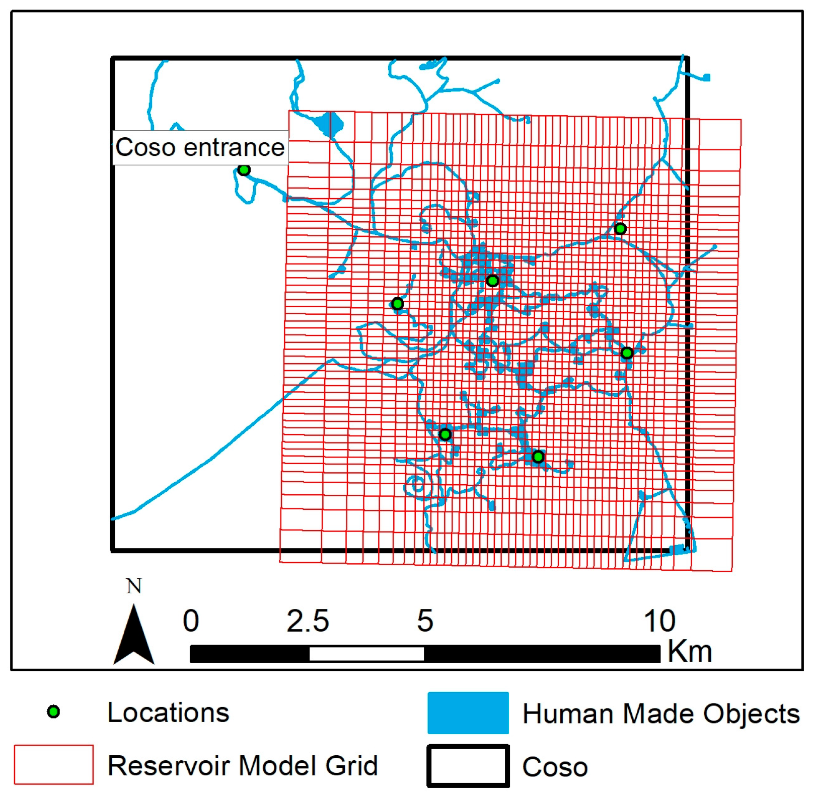
Reservoir model data have voxels with variable sizes. The grid direction and the coordinate system of the reservoir model do not match the data structure we used in this study. We matched reservoir model data to the surface data. We created a surface projection of the reservoir model structure, which consists of adjacent rectangles, as shown in Figure 5. The reservoir model projection does not align with the Coso area of interest (AOI) and appears to have a small rotation angle that needs adjustment. Also, the voxels are not square as expected. The voxel surface projection map helps to geolocate voxels and match them with the Coso AOI. We used the Coso AOI intersection and the voxel surface projection map. Non-intersecting sections of the voxel surface projection map are removed since they are out of the Coso AOI. The areas in the Coso AOI but not in the voxel surface projection map are assumed to be “Non-Geothermal” areas.
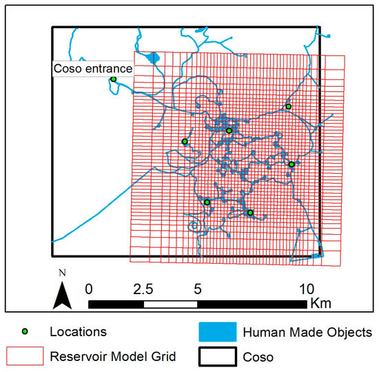
Figure 5.
Surface projection of reservoir model voxels.
2.3. Pattern Analysis
We conducted pattern analysis for each indicator using appropriate ML algorithms. Each indicator requires a different approach, explained in detail in the following subsections. LST pattern analysis mainly involves clustering analyses and interpolation. Fault pattern analyses consider every pixel’s distance to fault lines and to fault intersection points. Mineral marker pattern analyses are based on the fusion of various target detection algorithms to obtain an alteration mineral map intensity.
2.3.1. LST Pattern Analysis
The literature review indicates that geothermal resources exhibit distinct surface temperature patterns. Various clustering techniques, such as SOM and k-means clustering, have been employed in previous studies for time-series and clustering analyses of spatial data, demonstrating their effectiveness [10,21]. We employed the k-means clustering and SOM algorithm using LANDSAT images for CGF. In addition, we have applied kriging to the 2 m temperature probe data collected at CGF from 2017 to 2020.
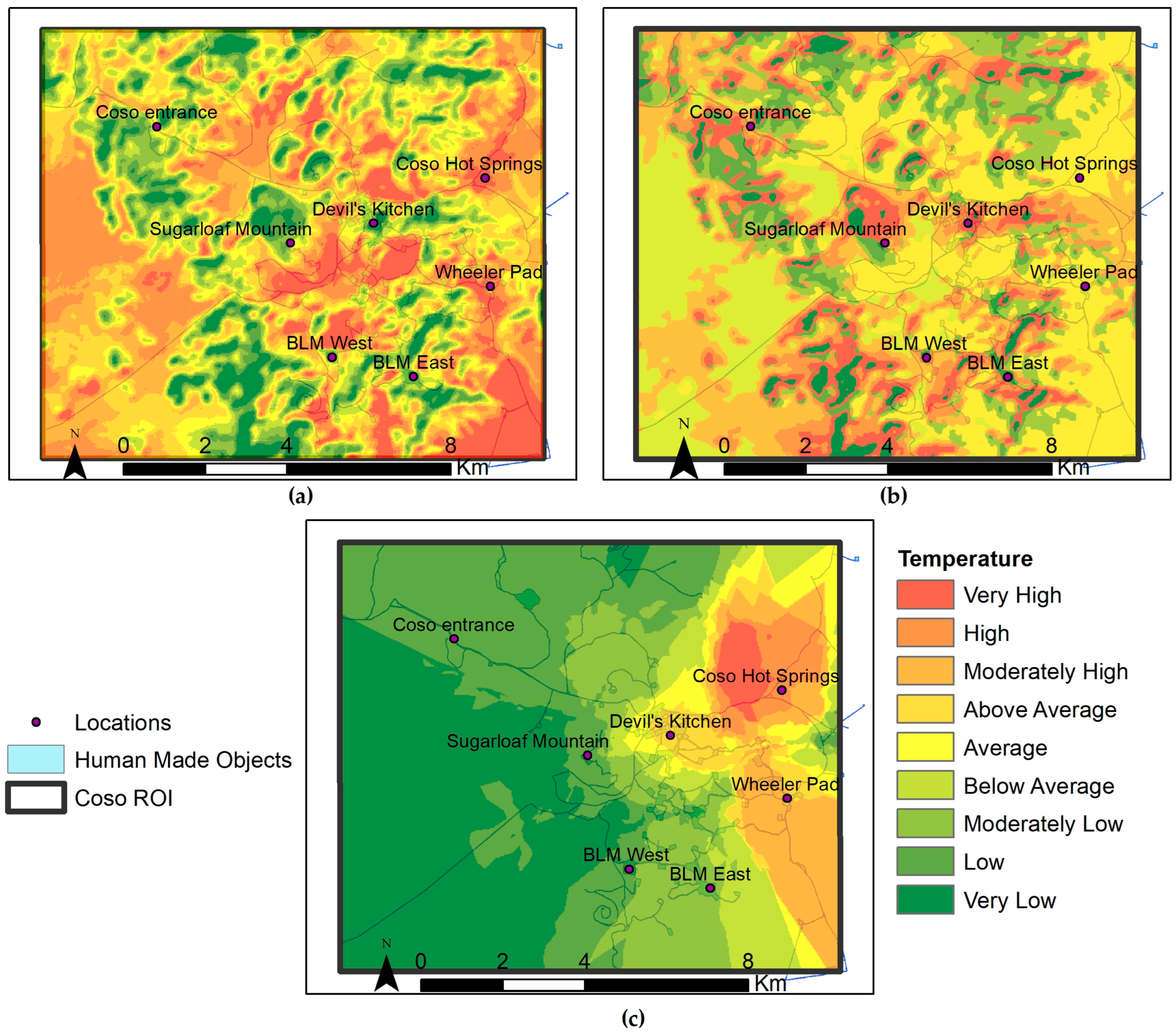
We applied several algorithms to test AI prediction, including SOM, kriging, nearest neighbor, and inverse distance weighted (IDW) algorithms. Finally, we used the k-means clustering algorithm on temperature data by comparing their accuracy. K-means clustering is a well-known unsupervised ML algorithm for spatial pattern extraction, which calculates centroids and assigns data points to the nearest centroid based on distance metrics. By applying k-means clustering, we identified persistently hot zones in the selected sites. Our dynamic analysis focuses on temporal anomalies and remains valid irrespective of climate, weather, or seasonality due to the persistent nature of hot zones. We have improved the k-means clustering method used by LST mapping utilizing a fixed (k = 5) k value [21]. We first apply the k-means clustering algorithm to all images with k values from 2 to 20, assuming each image has clusters of less than 20 separately. We have determined the best k value for each image using the elbow method [48]. Each image is clustered with the best k value. We generate k levels equally distributed to the lowest value equal to zero and the highest value equal to one. All cluster members (pixels) are mapped to a level value generated between zero and one. For example, for k = 5, if a pixel is in the cluster with the highest cluster center value, one is assigned to the pixel value; if a pixel is in the cluster with the second-highest cluster center value, 0.75 is assigned to the pixel value, and so on. Finally, we took an average of 85 images. Eventually, we have a normalized LST map. Figure 6a shows the k-means clustered temperature map. We have also applied SOM 3 × 3 analysis over the same set of images to compare the SOM results with variable k-means clustering results (Figure 6b). Besides, since we have 2 m temperature probe data, we created a temperature layer map using the kriging algorithm for these point data shown in Figure 6c.
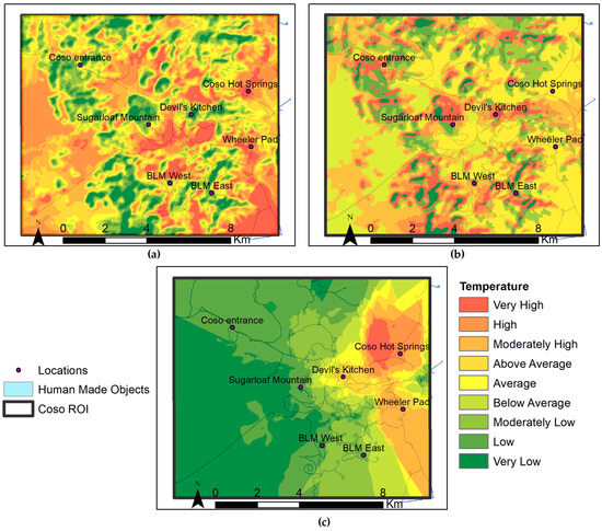
Figure 6.
Temperature maps: (a) K-means clustering; (b) 3 × 3 SOM; (c) Kriging.
2.3.2. Fault Pattern Analysis
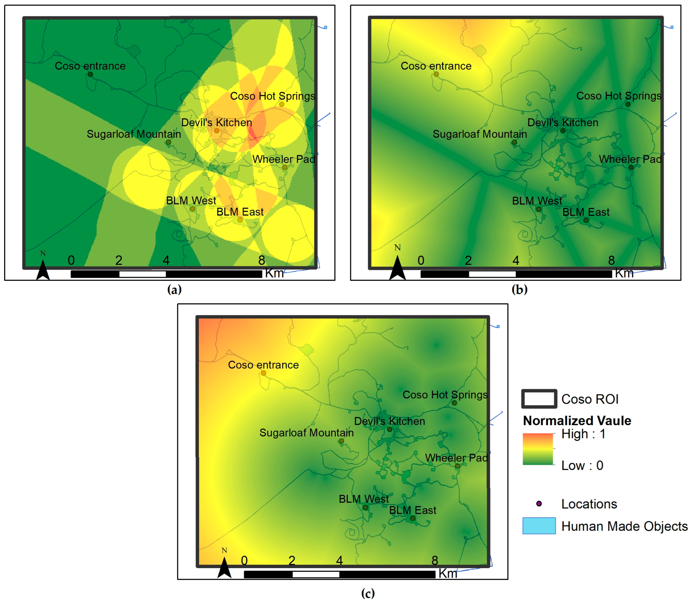
The layout and strength of the faults display distinctive attributes of geothermal resources. We acquired a fault map for CGF in shapefiles, depicting faults as linear features. We transformed fault lines into a density map (Figure 7a) to integrate the effect region of the faults into the geothermal AI system. In addition, alternative methods for analyzing faults have been studied. We have created the line distance fault map of CGF that calculates the minimum distance to fault lines (Figure 7b). We also determined the intersection points of fault lines, as shown in Figure 4. Then, we calculated the intersection point distance to the fault map of CGF, which calculates the minimum distance to the intersection points of fault lines. The point distance fault map is shown in Figure 7c. Comparison of these three results will be discussed in further sections.
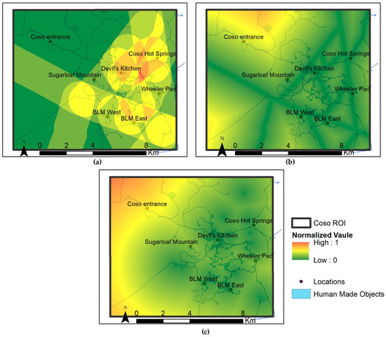
Figure 7.
Fault pattern maps: (a) Density; (b) Line distance; (c) Intersection point distance.
2.3.3. Mineral Markers Pattern Analysis
Alteration minerals are formed when minerals are exposed to water at high temperatures, often surfacing through faults, hot springs, and fumaroles. These minerals carry chemical signatures that reflect the characteristics of the underground system [49,50]. Geothermal fluid discharge on the surface can create deposits of various minerals like siliceous sinters, travertine [51], borates [52], sulfates, chlorides [53], calcite, and quartz, which form at temperatures ranging from 100 to over 300 degrees Celsius [54]. In some geothermal areas, the occurrence of minerals like kaolinite, calcite (tufa) [32,55], sinter deposits (opal-A, opal-CT, chalcedony, and quartz), hematite, epsomite, and gypsum has been documented [56]. These studies selected certain minerals indicating geothermal alteration based on their presence in the selected sites and the availability of their spectral signatures in the USGS Spectral Library. These include chalcedony, opal, kaolinite, hematite, and alunite. chalcedony, opal, kaolinite, and hematite spectra were used for spectral analysis to generate maps indicating the presence of these minerals. Hyperspectral satellite images were utilized, and the ENVI 5.7 software package was employed for target detection using eight algorithms. These algorithms include Adaptive Coherence Estimator (ACE), Constrained Energy Minimization (CEM), Matched Filtering (MF), Orthogonal Subspace Projection (OSP), Spectral Angle Mapper (SAM), Mixture Tuned Matched Filtering (MTMF), Target-Constrained Interference-Minimized Filter (TCIMF), and Mixture Tuned Target-Constrained Interference-Minimized Filter (MTTCIMF). The resulting mineral maps from each method were fused using a voting process to generate a consolidated “Mineral Markers” map indicating the presence of alteration minerals in the area [57].
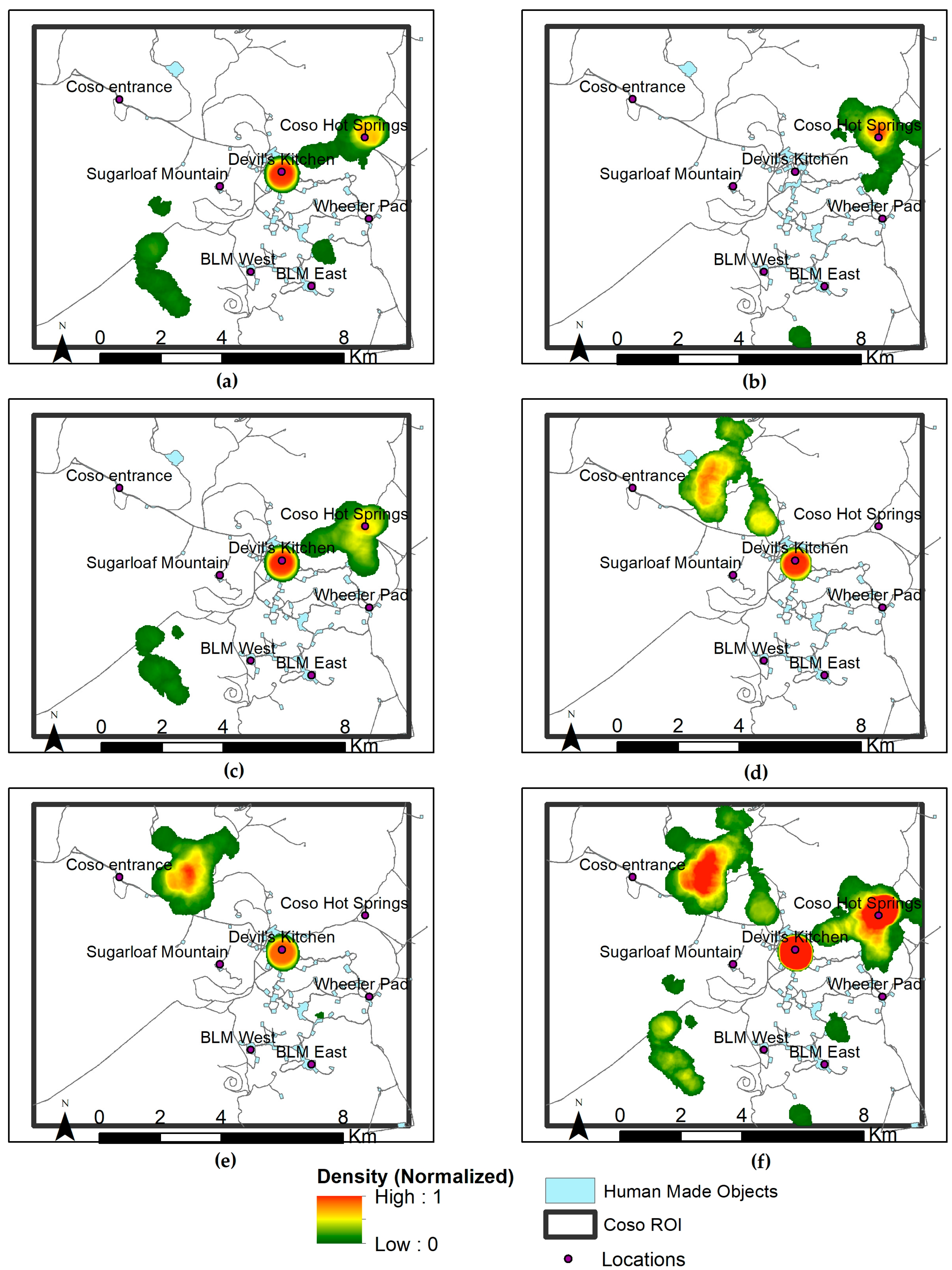
Laboratory measurements have been conducted to obtain the mineral content identification to ascertain the mineral composition of the samples. Using the geolocations of the samples and mineral occurrences, we measured the mineral maps’ accuracy by comparing each mineral’s occurrence for 97 samples and the mineral map values where samples are collected. The accuracy evaluation is also possible for mineral density maps. The advantage of using a density map is that accuracy can be increased by changing the density radius while creating a density map with an appropriate density radius. We analyzed each mineral alteration separately in eight different algorithms. We calculated the accuracy of each algorithm and the fusion of these algorithms. We concluded that the fusion of algorithms is better than using individuals. Therefore, we selected different numbers and types of mineral mapping algorithms concerning their accuracies for various minerals for fusion. Finally, since all these minerals are indicators of geothermal activity, we fused the fusion of these mineral maps as an input for geothermal AI (Figure 8).
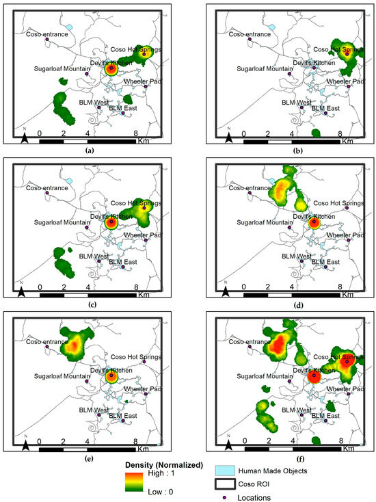
Figure 8.
Mineral density maps: (a) Alunite density map; (b) Hematite density map; (c) Kaolinite density map; (d) Chalcedony density map; (e) Opal density map; (f) Mineral density fusion map.
2.4. Labeling
Assigning labels to the geothermal system is challenging due to the uncertainty and professional analysis requirements. We started from the reservoir model to obtain the labels. The reservoir model has a 3-dimensional scheme. We took the footprint of this 3-dimensional scheme onto the surface level with the help of the surface projection of the reservoir model voxel structure map shown in Figure 5. Finally, we extended geothermal existence areas by injection and production well existence, so that all injection and production wells are covered within the “Geothermal” labeled zone. The result of the labeling algorithm used as the ground truth map is shown in Figure 9a. Brady and Desert Peak geothermal sites’ ground truth maps are shown in Figure 9b,c [21].
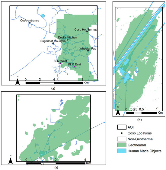
Figure 9.
Ground truth map of all fields: (a) Coso geothermal; (b) Brady geothermal; (c) Desert Peak geothermal.
All input (temperature, fault, and mineral) layers and the output ground truth layers for all sites (Brady, Coso, and Desert Peak) are resampled with a 3 × 3 m pixel size. The characteristics of Brady, Coso, and Desert Peak AOI datasets are listed in Table 3.

Table 3.
List of datasets.
2.5. Deep Learning Model (DLM)
In this study, we considered the AI model proposed by [21] since it has proven performance on the Brady and Desert Peak sites. However, we modified the proposed AI model as Coso has different data features and exhibits distinct geothermal features. We increased the convolution layer to 19 × 19 by adding 15 × 15, 17 × 17, and 19 × 19 convolution layers, while the AI model of Moraga et al. only has up to 13 × 13 convolution layers [21]. We also increased the input kernel size to 19 × 19 × 3, where the last dimension (×3) indicates the three layers: mineral, temperature, and fault, and 19 × 19 is the spatial distance that we focused on by setting the input data compatible with the internal design of the DLM architecture. The modified AI structure is shown in Figure 10.
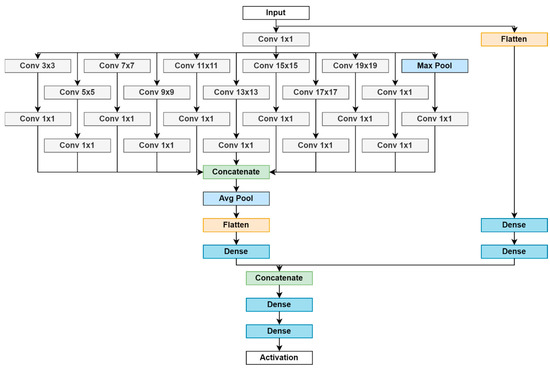
Figure 10.
Modified AI architecture.
Modified AI has layers that perform different functions described below.
Convolution Layer: The convolution layer implements a convolution operation that filters an image and matches the relevant image textures. Mathematically, the output of a convolution layer is calculated by Equation (1):
where is the input tensor, is the filter tensor, is the activation function, is the bias vector, and is the output tensor.
Dense Layer: A dense layer is a fully connected layer and can be mathematically interpreted as a matrix multiplication followed by a bias addition and activation function calculated by Equation (2).
where is the number of neurons in the dense layer, n is the number of input features, is the input vector, is the weight matrix, is the activation function, is the bias vector, and is the output tensor.
Max Pooling Layer: For each position in the output tensor, the max pooling operation computes the maximum value of the elements in the corresponding window of the input tensor.
Average Pooling Layer: For each position in the output tensor, the average pooling operation computes the average value of the elements in the corresponding window of the input tensor.
Flatten Layer: The flatten layer reduces the dimensionality of the inputs and turns them into a single-dimensional array.
Concatenate Layer: The Concatenate layer merges the input data into one single output.
Activation Layer: We used the SoftMax activation function at the final step since geothermal AI is a classification model.
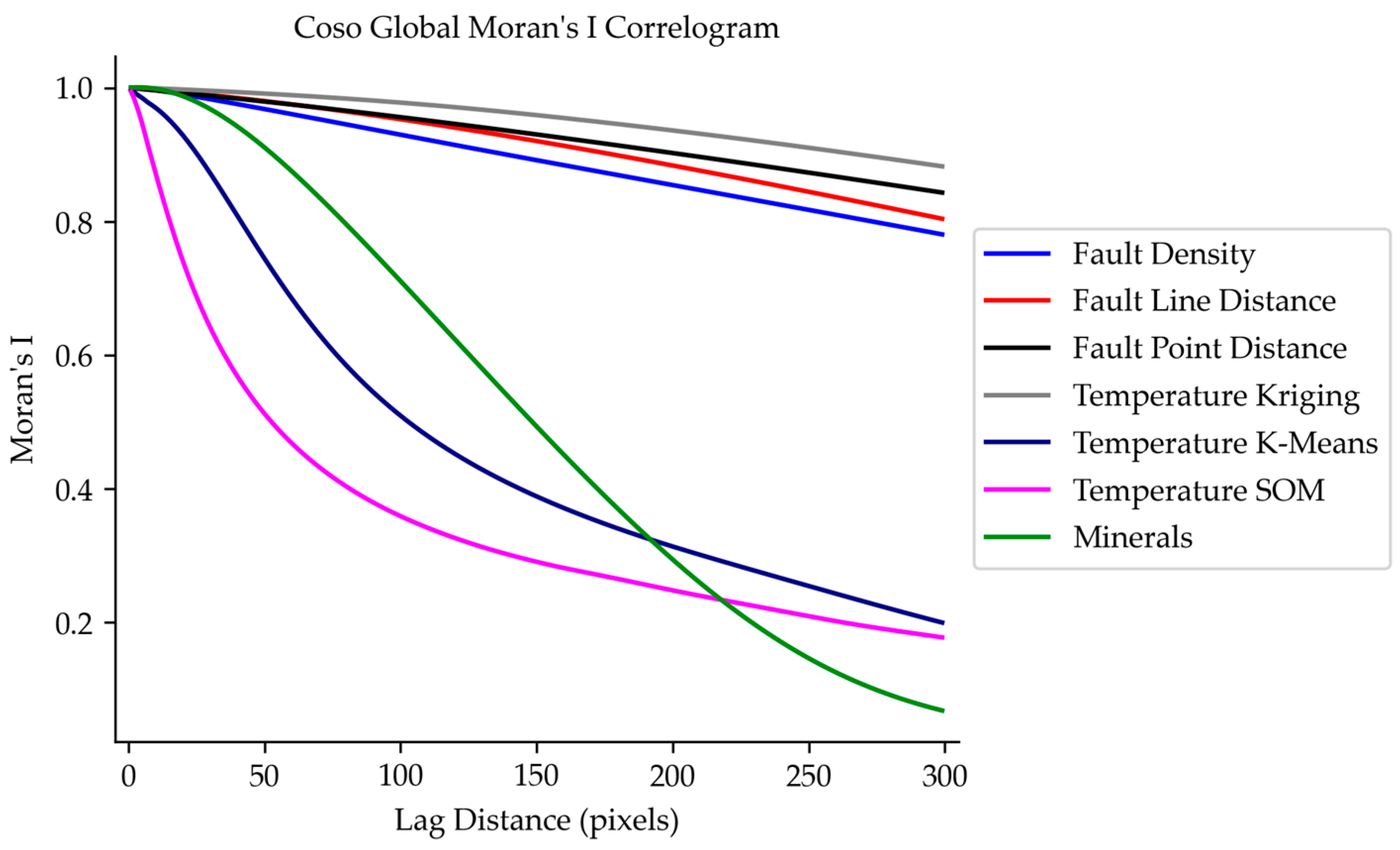
The increased convolutional layers are due to the increased spatial correlation with the addition of Coso data. Moran’s I is the typical measure of spatial correlation, and its values for different lag sizes in a correlogram for temperature, fault, and mineral layers of Coso are given in Figure 11. Each pixel in Figure 11 shows a positive connection with neighboring pixels within a lag of up to 13. Figure 11 shows that all indicators exhibit positive autocorrelation, which decreases with distance. The SOM and k-means temperature indicators sharply decrease by pixel 19, whereas the mineral marker indicators show an inflection point around pixel 50 in both sites. The result indicates that the autocorrelation is more pronounced up to a pixel between 19 and 50, which was incorporated into the modified AI architecture.
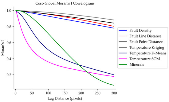
Figure 11.
Correlogram of geothermal indicators for Coso geothermal field.
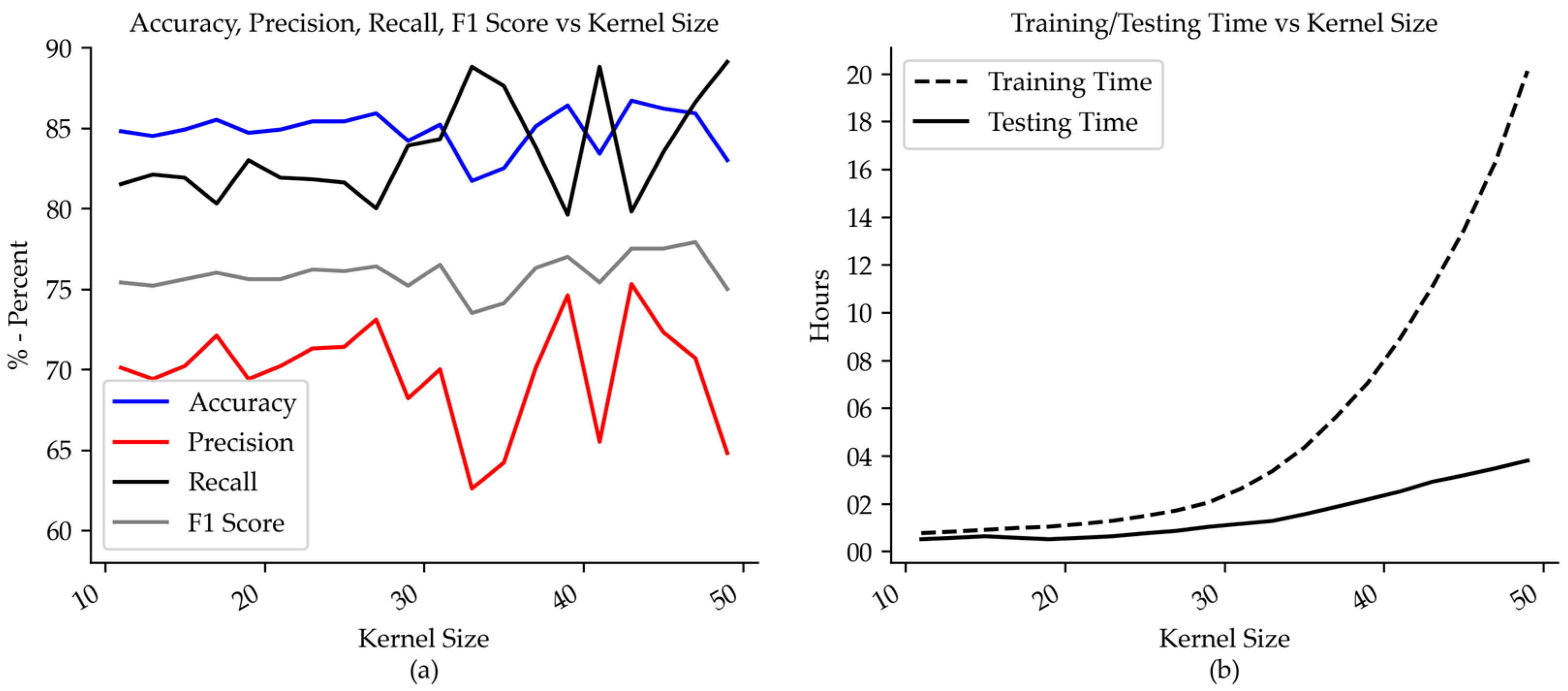
In addition to autocorrelation analysis, we trained the model with increasing kernel sizes to navigate the effects of kernel size on the results. Figure 12 shows the training set’s kernel size vs. accuracy, precision, recall, and F1 score. It is also interpreted from Figure 12 that training time increases exponentially, although no significant improvement has been observed in accuracy, recall, precision, and F1 score values. After the kernel size reached 19, a sudden jump in the training time was observed. Based on the analyses above, we can infer that the autocorrelation is stronger up to pixel 19, which was used as an input in the architecture design of the modified AI model.

Figure 12.
Effect of kernel size on training: (a) Accuracy, precision, recall, and F1 score vs. kernel size graph; (b) Training/testing time vs. kernel size graph.
We have used High-Performance Computing (HPC) resources of Colorado School of Mines, with two on-premise GPU workstations: 256 GB RAM and three NVIDIA RTX A 5000 GPUs, and 1024 GB RAM and two NVIDIA RTX 6000 Ada GPUs. Both workstations have the Ubuntu 20.04 operating system and the CUDA 12.2 Library.
3. Analysis and Discussion
We resampled all datasets of the three sites to a 3 × 3 m pixel size. Coso AOI has a total of 14,381,640 pixels; 10,270,255 of them are labeled as “Non-Geothermal”, and 4,111,385 of them are labeled as “Geothermal”. We have three options for the temperature layer created using kriging, k-means clustering, and SOM algorithms. Meanwhile, three fault layers were created using KDE, line distance, and line intersection point distance methods. We have a single mineral layer to use as input to DLM. These combinations yield nine datasets for training and testing AI models. The combinations of datasets are as follows:
Fault Density–Temperature Kriging (DK): This is the dataset where the fault density map is used as the fault layer, the temperature kriging map is used as the temperature layer, and the mineral map is used as the mineral layer.
Fault Density–Temperature K-means (DM): This is the dataset where the fault density map is used as the fault layer, the temperature k-means clustering map is used as the temperature layer, and the mineral map is used as the mineral layer.
Fault Density–Temperature SOM (DS): This is the dataset where the fault density map is used as the fault layer, the temperature SOM 3 × 3 map is used as the temperature layer, and the mineral map is used as the mineral layer.
Fault Line Distance–Temperature Kriging (LK): This is the dataset where the fault line distance map is used as the fault layer, the temperature kriging map is used as the temperature layer, and the mineral map is used as the mineral layer.
Fault Line Distance–Temperature K-means (LM): This is the dataset where the fault line distance map is used as the fault layer, the temperature k-means clustering map is used as the temperature layer, and the mineral map is used as the mineral layer.
Fault Line Distance–Temperature SOM (LS): This is the dataset where the fault line distance map is used as the fault layer, the temperature SOM 3 × 3 map is used as the temperature layer, and the mineral map is used as the mineral layer.
Fault Point Distance–Temperature Kriging (PK): This is the dataset where the fault intersection point distance map is used as the fault layer, the temperature kriging map is used as the temperature layer, and the mineral map is used as the mineral layer.
Fault Point Distance–Temperature K-means (PM): This is the dataset where the fault intersection point distance map is used as the fault layer, the temperature k-means clustering map is used as the temperature layer, and the mineral map is used as the mineral layer.
Fault Point Distance–Temperature SOM (PS): This is the dataset where the fault intersection point distance map is used as the fault layer, the temperature SOM 3 × 3 map is used as the temperature layer, and the mineral map is used as the mineral layer.
We have trained the models with 50,000 “Geothermal” labeled random samples, which is 1.2% of the “Geothermal” labeled set, and 50,000 “Non-Geothermal” labeled random samples, which is 0.5% of the “Non-Geothermal” labeled set, with a total of 100,000 samples from each dataset, which is 0.7% of the entire dataset. Finally, we conducted self-tests of these models over the Coso AOI; the accuracy results are shown in Table 4. The DK and PK models have the highest AUC values and accuracies, respectively.

Table 4.
DLM results of fault and temperature patterns of Coso geothermal field (bold values indicates best performing values).
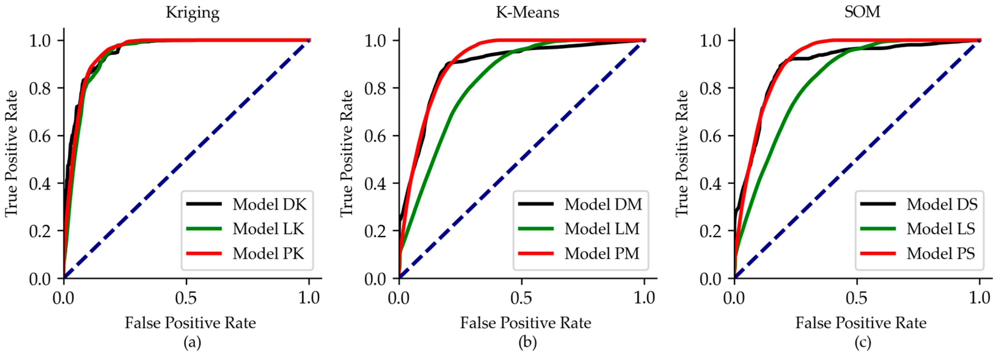
Another way of evaluating the performance of a binary classification model is the receiver operating characteristic (ROC) curve. An ROC curve is a graphical representation that illustrates the performance of a binary classification model across different discrimination thresholds. It is created by plotting the true positive rate (TPR) against the false positive rate (FPR) at various threshold settings. The area under the ROC Curve (AUC) indicates the model’s discrimination ability. Figure 13 shows the ROC curves, and Table 4 shows the corresponding AUC values of each model. By assessing the accuracies and AUC values together, both Fault Density–Temp. Kriging (DK) and Fault Point Dist.–Temp. Krig. (PK) perform best, where PK is slightly better in accuracy and DK is slightly better in AUC. We have selected Fault Density–Temp. Kriging (DK) as the best-performing dataset for the Coso AOI. The kriging temperature map and fault density map will be used as inputs for Coso in the next chapters of this study.
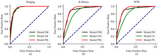
Figure 13.
ROC curves of Coso models; (a) Kriging; (b) K-means; (c) SOM.
3.1. Comparison of Three Geothermal Sites
We have compared three geothermal sites: Brady, Coso, and Desert Peak. The datasets of each geothermal site are listed in Table 3. We trained seven models to investigate the transferability of models.
Model B: The model trained with 50,000 (15.5%) “Geothermal” labeled random samples and 50,000 (22.7%) “Non-Geothermal” labeled random samples, with a total of 100,000 (16.9%) samples, from Brady.
Model C: The model trained with 50,000 (1.2%) “Geothermal” labeled random samples and 50,000 (0.5%) “Non-Geothermal” labeled random samples, with a total of 100,000 (0.7%) samples, from Coso.
Model D: The model trained with 50,000 (4.1%) “Geothermal” labeled random samples and 50,000 (3.8%) “Non-Geothermal” labeled random samples, with a total of 100,000 (3.9%) samples, from Desert Peak.
Model BC: The model trained with 50,000 (15.5%) “Geothermal” labeled random samples and 50,000 (22.7%) “Non-Geothermal” labeled random samples, with a total of 100,000 (16.9%) samples, from Brady, and 50,000 (1.2%) “Geothermal” labeled random samples and 50,000 (0.5%) “Non-Geothermal” labeled random samples, with a total of 100,000 (0.7%) samples, from Coso.
Model BD: The model trained with 50,000 (15.5%) “Geothermal” labeled random samples and 50,000 (22.7%) “Non-Geothermal” labeled random samples, with a total of 100,000 (16.9%) samples from Brady, and 50,000 (4.1%) “Geothermal” labeled random samples and 50,000 (3.8%) “Non-Geothermal” labeled random samples, with a total of 100,000 (3.9%) samples, from Desert Peak.
Model CD: The model trained with 50,000 (1.2%) “Geothermal” labeled random samples and 50,000 (0.5%) “Non-Geothermal” labeled random samples, with a total of 100,000 (0.7%) samples from Coso, and 50,000 (4.1%) “Geothermal” labeled random samples and 50,000 (3.8%) “Non-Geothermal” labeled random samples, with a total of 100,000 (3.9%) samples, from Desert Peak.
Model BCD: The model trained with 50,000 (15.5%) “Geothermal” labeled random samples and 50,000 (22.7%) “Non-Geothermal” labeled random samples, with a total of 100,000 (16.9%) samples from Brady, 50,000 (1.2%) “Geothermal” labeled random samples and 50,000 (0.5%) “Non-Geothermal” labeled random samples, with a total of 100,000 (0.7%) samples from Coso, and 50,000 (4.1%) “Geothermal” labeled random samples, and 50,000 (3.8%) “Non-Geothermal” labeled random samples, with a total of 100,000 (3.9%) samples, from Desert Peak.
The seven models described above are summarized in Table 5. We have tested these models on Brady, Coso, and Desert Peak geothermal sites. Twenty-one prediction results are evaluated. We have studied these results in three groups: self-testing, dependent testing, and independent testing. Self-testing means that a model is trained for a given site and is tested for the same site. Models B, C, and D are the self-tested models. The addition of external data in the training and testing of models is called dependent testing. Models are trained with samples from at least two sites. It reveals how the models change by adding data from another site to the training set. For example, for the test of the Brady geothermal site, model BD, model BC, and model BCD are the dependent models. The independent testing involves evaluating each model on sites trained for a different location. Model C, model D, and model CD are considered independent models for the independent test of the Brady geothermal site because they are not trained using any data from the Brady site.

Table 5.
The list of trained models used three geothermal fields.
3.1.1. Self-Testing
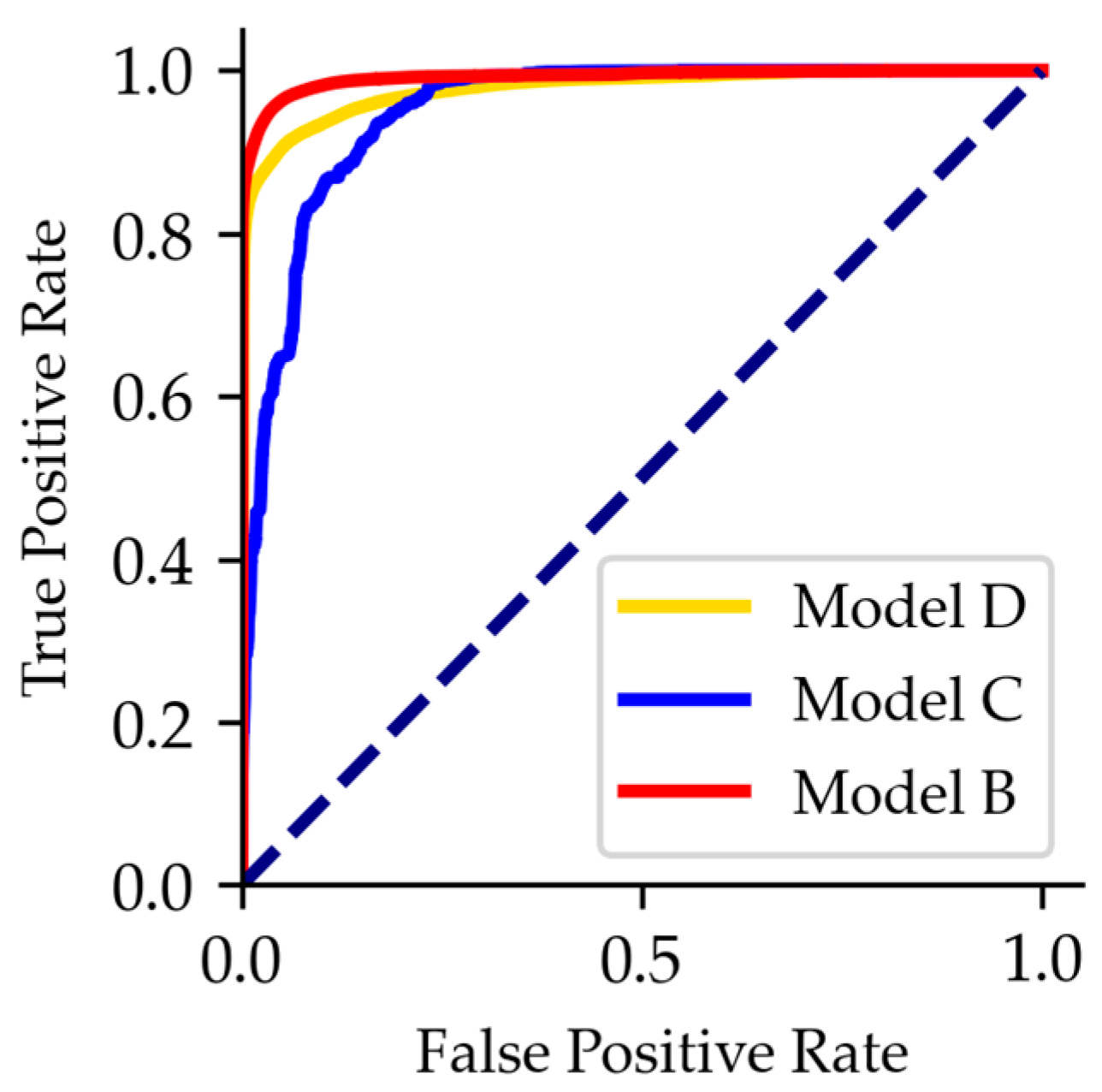
Since this is self-testing, the performance is expected to be higher than any other test site. The accuracy of model B is 96%, the accuracy of model C is 87%, and the accuracy of model D is 93%. Model C has a slightly lower precision, which indicates an increase in false negatives. The performance metrics of self-testing are given in Table 6. The ROC curves of self-testing are shown in Figure 14.

Table 6.
Performance of the modified AI for the selected sites for self-testing.

Figure 14.
ROC curves of self-testing.
Model C also has an AUC value of 0.951, which shows a significantly high discrimination ability. Model B has an AUC value almost equal to 0.991, which shows a perfect discrimination ability. Model D has an AUC value of 0.978, between the C and B AUC values.
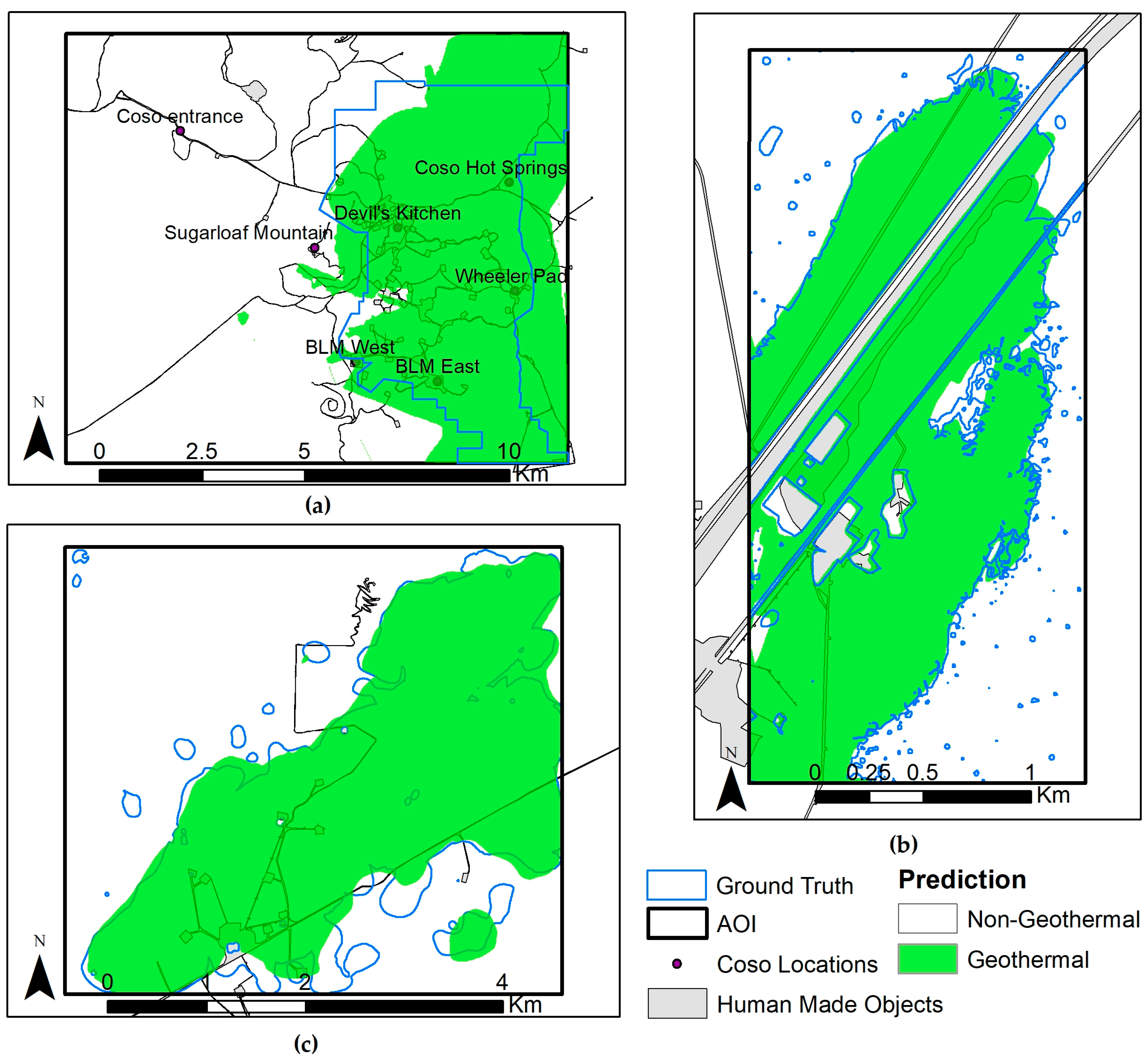
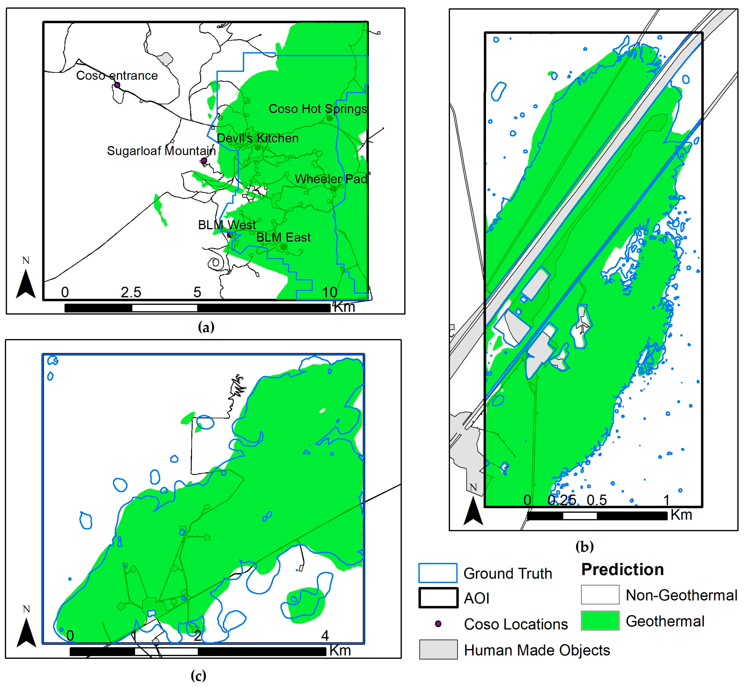
Figure 15 shows the prediction maps of model C, model B, and model D, respectively. The predicted geothermal fields overlap the operational geothermal areas in all three models. The quality metrics mentioned above and the visual representation of the maps ensure that the models for self-testing are working very well.
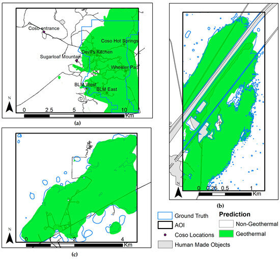
Figure 15.
Prediction maps of self-testing: (a) model C applied to Coso; (b) model B applied to Brady; (c) model D applied to Desert Peak.
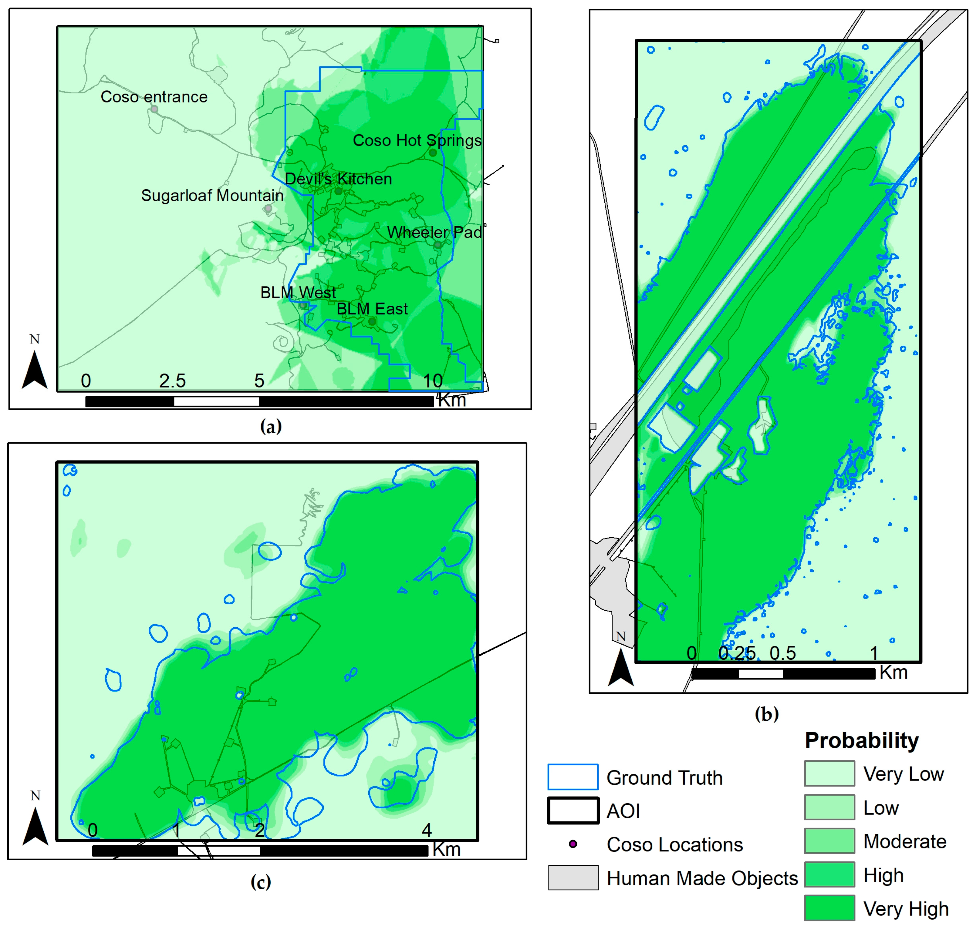
A probability map is another way of visualizing and evaluating the performance of test results. The probability maps verify how well models fit with the ground truths. Probability results are classified into five sets concerning the probability of being classified as “Geothermal”: namely, very high, high, moderate, low, and very low, with equal probability ranges. Probability maps provide the geographic locations that are about to be classified as “Geothermal” although they are classified as “Non-Geothermal”, or vice versa. They bring a powerful insight into the characteristics of the model. Figure 16 shows the probability maps of model C, model B, and model D, respectively. The prediction maps reveal the probability of the model being distributed over the entire area.

Figure 16.
Probability maps of self-testing: (a) model C applied to Coso; (b) model B applied to Brady; (c) model D applied to Desert Peak.
3.1.2. Dependent Testing
In this test, some external data is added to the test sets. Models are trained with samples from at least two sites. Model BD, model BC, and model BCD are the dependent models for the Brady geothermal site test. Similarly, model BC, model CD, and model BCD are dependent models of CGF, and model BD, model CD, and model BCD are dependent models of Desert Peak. Table 7 shows the performance of dependent tests based on AUC, accuracy, precision, and recall metrics. As expected for dependent testing, the accuracies are over 85% in all models. The results of the dependent models are also satisfactory, like the self-testing models.

Table 7.
Dependent test performance of geothermal AI (bold values indicates best performing values).
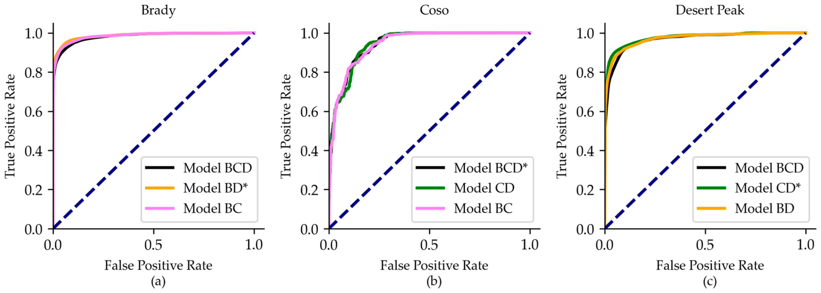
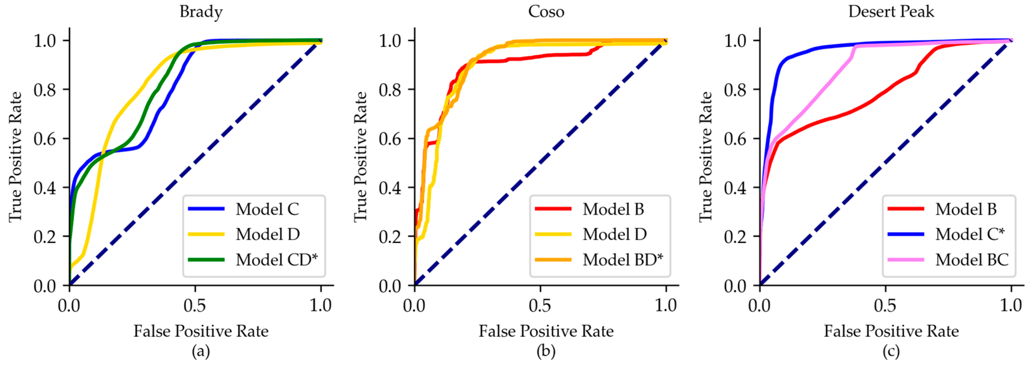
Figure 17 shows the ROC curves of dependent tests. Model BD applied to Brady, model CD applied to Coso, and model CD applied to Desert Peak are the best-performing dependent tests for the sites Brady, Coso, and Desert Peak, respectively.
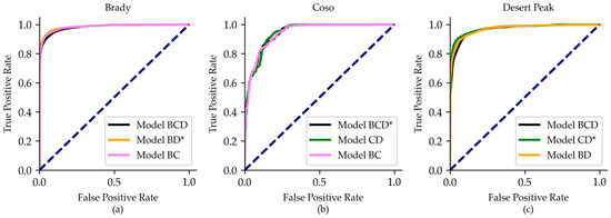
Figure 17.
ROC curves of dependent tests for (* indicates best-performing models): (a) Brady; (b) Coso; (c) Desert Peak.
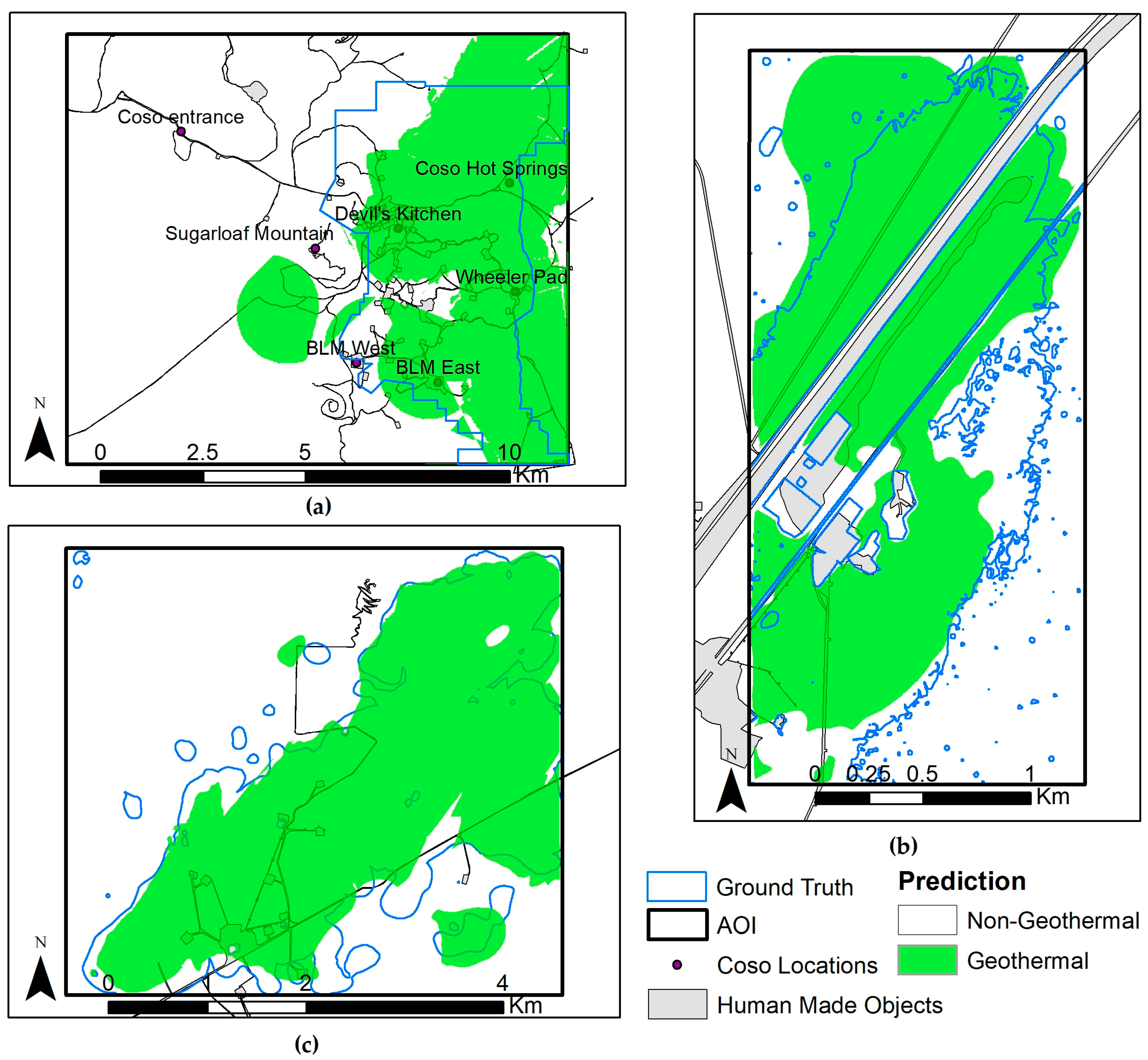
Prediction maps of the best-performing dependent tests are shown in Figure 18. Coso’s best-performing dependent prediction map predicts additional “Geothermal” areas north of Devil’s Kitchen and west of Wheeler Pad. It predicts additional “Non-Geothermal” areas south of Sugarloaf Mountain compared to Coso’s self-testing. The best performing dependent prediction maps of Brady and Desert Peak are almost in line with the self-testing of Brady and Desert Peak, respectively.
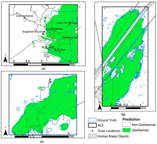
Figure 18.
Prediction maps of best-performing dependent tests: (a) model CD applied to Coso; (b) model BD applied to Brady; (c) model CD applied to Desert Peak.
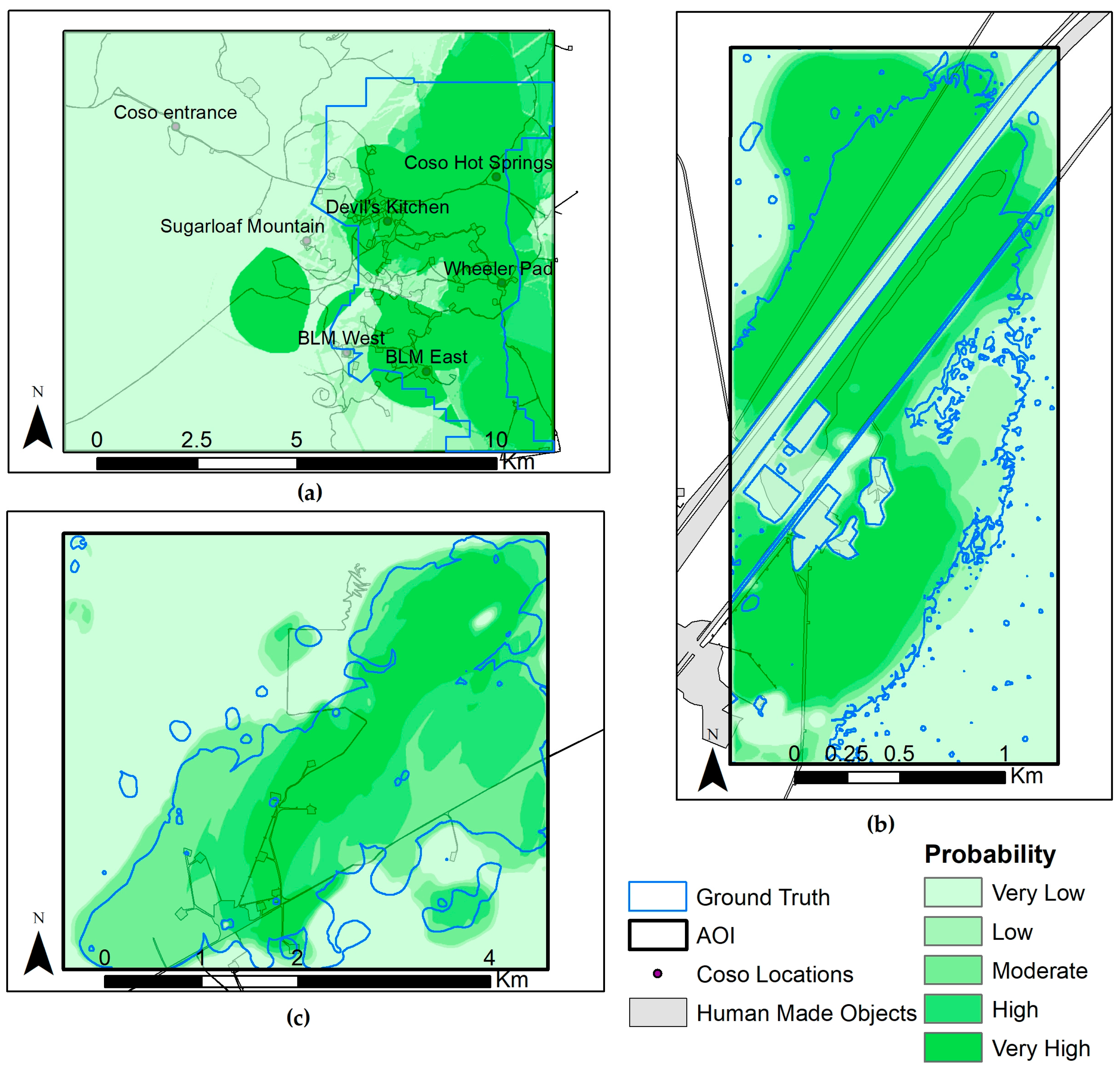
Figure 19 shows probability maps of the best-performing dependent tests. Devil’s Kitchen, Wheeler Pad, Coso Hot Springs, and BLM East are high-probability concentrated points in the best-performing dependent test of Coso. The best-performing dependent tests of Brady and Desert Peak overlap with the ground truths of these maps.
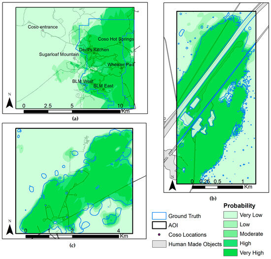
Figure 19.
Probability maps of best-performing dependent tests: (a) model CD applied to Coso; (b) model BD applied to Brady; (c) model CD applied to Desert Peak.
3.1.3. Independent Testing
In the independent testing, each model is tested on sites for which it was not trained. Model C, model D, and model CD are the independent models for the Brady geothermal site test. Similarly, model B, model D, and model BD are independent models for Coso, and model B, model C, and model BC are independent models for Desert Peak. Model D applied to Brady is the best-performing independent test for Brady according to accuracy (75%), and model CD applied to Brady is the best-performing independent test for Brady according to AUC (0.828). Model BD applied to Coso is the best-performing independent test for Coso, with 82% accuracy and 0.914 AUC values, respectively. Model C applied to Desert Peak is the best-performing independent test for Desert Peak, with 90% accuracy and 0.953 AUC values, respectively. Table 8 shows the performance of dependent tests based on AUC, accuracy, precision, and recall metrics.

Table 8.
Independent test performance of geothermal AI (bold values indicates best performing values for each geothermal site).
Five of six cross-tests (model B applied to Coso, model B applied to Desert Peak, model C applied to Brady, model C applied to Desert Peak, model D applied to Brady, and model D applied to Coso) have accuracies better than 70%, except that model C applied to Brady has 64% accuracy.
When we looked at the ROC performances of the independent tests (Figure 20), the ROCs of model C and model CD applied to Brady have similar characteristics. Although model D applied to Brady has distinct characteristics, the AUC values of all three tests are very close. Coso’s ROCs have identical characteristics with slight differences in AUC values. Desert Peak’s ROCs have different characteristics. Model C applied to Desert Peak is the best ROC for Desert Peak.
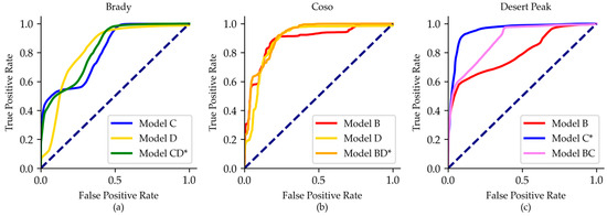
Figure 20.
ROC curves of independent tests for (* indicates best-performing models): (a) Brady; (b) Coso; (c) Desert Peak.
Prediction maps of the best-performing independent tests are shown in Figure 21. Coso’s best-performing independent prediction map predicts additional “Geothermal” areas southwest of Sugarloaf Mountain and northwest of BLM West and additional “Non-Geothermal” areas south of Devil’s Kitchen and north of BLM West and BLM East.

Figure 21.
Prediction maps of best-performing independent tests: (a) model BD applied to Coso; (b) model D applied to Brady; (c) model C applied to Desert Peak.
Probability maps of the best-performing independent tests are shown in Figure 22. An additional “Geothermal” area southwest of Sugarloaf Mountain and northwest of BLM West appears in the probability maps as a high-probability area.

Figure 22.
Probability maps of best-performing independent tests: (a) model BD applied to Coso; (b) model D applied to Brady; (c) model C applied to Desert Peak.
Pair tests are the two independent tests that are trained on one site and tested on the opposite site for any geothermal site pair. When accuracies of pair tests are higher than 80% and AUC values of pair tests are higher than 0.85, a geothermal site pair is called a cross-compatible site pair.
Brady and Coso pair tests (model C applied to Brady and model B applied to Coso) have 64% and 83% accuracies and have 0.811 and 0.888 AUC values, respectively, which are not high enough to evaluate them as cross-compatible.
Brady and Desert Peak pair tests (model D applied to Brady and model B applied to Desert Peak) have 75% and 72% accuracies and have 0.820 and 0.795 AUC values, respectively, which are not high enough to evaluate them as cross-compatible.
Coso and Desert Peak pair tests (model D applied to Coso and model C applied to Desert Peak) have 82% and 90% accuracies and have 0.889 and 0.953 AUC values, respectively, which are high enough to evaluate them as cross-compatible.
4. Conclusions
Our methodology combines RS, ML, and AI to forecast potential geothermal sites, applicable to both new explorations and the expansion of existing ones. By leveraging AI for predictive modeling and assessing cross-compatibility, our approach establishes a framework for globally applicable geothermal AI solutions.
Although geothermal indicators remain the same, pattern analysis of indicator data can enhance the efficiency and accuracy of the geothermal AI model. We have revealed that various patterns can be applied to geothermal indicators: mineral markers, temperature, and faults. Coso’s case study showed that local temperature probe data enhances the geothermal AI model, while LST from ASTER satellite data may not have been sufficient to delineate temperature indicator characteristics. Moreover, line and intersection point distances applied to fault data can be alternatives to KDE for fault indicator pattern analysis since corresponding geothermal AI models have comparable accuracies. Besides, using the fusion of mineral marker density maps is one of the novel aspects of this study, which shows the mineral marker pattern applied.
We explored the application of artificial intelligence (AI) models for geothermal site classification across three distinct geothermal fields: Brady, Coso, and Desert Peak. Our analysis focused on evaluating the performance of various models through self-testing, dependent testing, and independent testing phases, aiming to understand their predictive capabilities and cross-compatibility across different sites.
By leveraging known indicators such as mineral markers, surface temperature, and faults, our approach aims to overcome the limitations of site-specific AI applications. Through comprehensive testing across three distinct geothermal sites (Brady, Desert Peak, and Coso), we have demonstrated the feasibility of cross-compatibility between certain sites, enabling the transferability of AI models. This transferability of the proposed AI model is the most valuable finding of this study.
Models trained and tested on the same site demonstrated high accuracy and robust discrimination ability. Model B for Brady, model C for Coso, and model D for Desert Peak exhibited accuracy rates exceeding 87%, with area under the curve (AUC) values indicating excellent model discrimination.
Models trained with data from multiple sites maintained strong performance metrics, emphasizing their adaptability across geographically similar areas. Models BD and BC for Brady, models BD and D for Coso, and models C and CD for Desert Peak showcased accuracies above 85% and maintained competitive AUC values, reinforcing their reliability in varied geothermal contexts.
Evaluating models on sites for which they were not trained revealed nuanced performance. Model D for Brady, model BD for Coso, and model C for Desert Peak emerged as top performers, achieving accuracies ranging from 72% to 90% and demonstrating robust discrimination with AUC values above 0.8.
Visual representations (prediction and probability maps) of model predictions not only aligned closely with known geothermal features but also provided additional insights into model confidence levels. These maps validated the models’ efficacy in delineating geothermal and non-geothermal areas across the three sites, while also highlighting high-probability areas for geothermal presence and guiding further exploration efforts.
Pair tests evaluated cross-compatibility between sites based on model performance. While the Brady–Coso and Brady–Desert Peak pairs showed moderate performance in cross-site predictions, the Coso–Desert Peak pair demonstrated high cross-compatibility, suggesting the potential applicability of models trained on one site to predict geothermal features in another.
Our findings underscore that while certain geothermal sites (e.g., Desert Peak and Coso) share similar characteristics and thus have cross-compatible AI models, others (e.g., Brady) may not integrate as seamlessly. Understanding these nuances is crucial for the development and deployment of AI models in geothermal exploration.
By refining our methodology and expanding our research scope, we aim to further enhance the efficacy and global applicability of geothermal AI models. This study emphasizes the transformative potential of AI-driven approaches in advancing the exploration and sustainable exploitation of geothermal energy resources, contributing to a greener and more resilient energy future.
Furthermore, we will continue to develop AI models to understand the effect of each indicator. Moreover, we will study the impact of each pixel of each indicator to explain the patterns found in the proposed AI model.
Author Contributions
Conceptualization, E.D. and H.S.D.; methodology, E.D.; software, E.D. and M.C.; validation, E.D., H.S.D., Y.-T.Y. and M.C.; formal analysis, M.C. and H.S.D.; investigation, M.C., H.S.D., E.D. and Y.-T.Y.; resources, E.D., H.S.D., Y.-T.Y. and M.C.; data curation, M.C.; writing—original draft preparation, E.D.; writing—review and editing, E.D., M.C. and H.S.D.; visualization, E.D.; supervision, H.S.D.; project administration, H.S.D.; funding acquisition, H.S.D. All authors have read and agreed to the published version of the manuscript.
Funding
This research was funded by the US Department of Energy grant number DE-EE0008760, and the APC was funded by DE-EE0008760.
Data Availability Statement
Due to the presence of proprietary content, certain data and algorithms utilized in this research cannot be shared. However, the ones that are publicly available can be shared with others. Please reach out to the authors for any specific data or algorithm requirements.
Acknowledgments
We would like to thank NASA, USGS, the Navy Geothermal Program Office, and CSM for their support. We used high-performance computing (HPC) and other Colorado School of Mines facilities. We benefited from the availability of satellite data from NASA’s ASTER projects and USGS. Additionally, we would like to thank Coso Operating Company in California for their support and valuable feedback.
Conflicts of Interest
The authors declare no conflicts of interest. The funders had no role in the design of the study; in the collection, analyses, or interpretation of data; in the writing of the manuscript; or in the decision to publish the results.
References
- Messerli, P.; Murniningtyas, E.; Eloundou-Enyegue, P.; Foli, E.G.; Furman, E.; Glassman, A.; Licona, G.H.; Kim, E.M.; Lutz, W.; Moatti, J.-P.; et al. Global Sustainable Development Report 2019: The Future Is Now–Science for Achieving Sustainable Development; United Nations Department of Economic and Social Affairs: New York, NY, USA, 2019. [Google Scholar]
- Domra Kana, J.; Djongyang, N.; Raïdandi, D.; Njandjock Nouck, P.; Dadjé, A. A review of geophysical methods for geothermal exploration. Renew. Sustain. Energy Rev. 2015, 44, 87–95. [Google Scholar] [CrossRef]
- Warner, N.R.; Darrah, T.H.; Jackson, R.B.; Millot, R.; Kloppmann, W.; Vengosh, A. New Tracers Identify Hydraulic Fracturing Fluids and Accidental Releases from Oil and Gas Operations. Environ. Sci. Technol. 2014, 48, 12552–12560. [Google Scholar] [CrossRef] [PubMed]
- Lo, T.; Inderwiesen, P.L. Fundamentals of Seismic Tomography; Society of Exploration Geophysicists: Houston, TX, USA, 1994. [Google Scholar] [CrossRef]
- Yu, G.; Bryans, B.W.; Ju, C.; Liang, B.; Zhou, F. High-resolution crosswell seismic imaging in JiangSu Oilfield, China. In SEG Technical Program Expanded Abstracts 2003; Society of Exploration Geophysicists: Houston, TX, USA, 2005; pp. 2251–2254. [Google Scholar] [CrossRef]
- Lukawski, M.Z.; Silverman, R.L.; Tester, J.W. Uncertainty analysis of geothermal well drilling and completion costs. Geothermics 2016, 64, 382–391. [Google Scholar] [CrossRef]
- Reath, K.A.; Ramsey, M.S. Exploration of geothermal systems using hyperspectral thermal infrared remote sensing. J. Volcanol. Geotherm. Res. 2013, 265, 27–38. [Google Scholar] [CrossRef]
- Sekertekin, A.; Arslan, N. Monitoring thermal anomaly and radiative heat flux using thermal infrared satellite imagery—A case study at Tuzla geothermal region. Geothermics 2019, 78, 243–254. [Google Scholar] [CrossRef]
- Calvin, W.M.; Littlefield, E.F.; Kratt, C. Remote sensing of geothermal-related minerals for resource exploration in Nevada. Geothermics 2015, 53, 517–526. [Google Scholar] [CrossRef]
- Cavur, M.; Moraga, J.; Duzgun, H.S.; Soydan, H.; Jin, G. The DInSAR Analysis with Machine Learning for Delineating Geothermal Sites at the Brady Geothermal Field. In Proceedings of the 46th Workshop on Geothermal Reservoir Engineering, Stanford, CA, USA, 16–18 February 2021. [Google Scholar]
- Qin, Q.; Zhang, N.; Nan, P.; Chai, L. Geothermal area detection using Landsat ETM+ thermal infrared data and its mechanistic analysis—A case study in Tengchong, China. Int. J. Appl. Earth Obs. Geoinf. 2011, 13, 552–559. [Google Scholar] [CrossRef]
- Hodder, D.T. Application of remote sensing to geothermal prospecting. Geothermics 1970, 2, 368–380. [Google Scholar] [CrossRef]
- Sabins, F.F. Remote sensing for mineral exploration. Ore Geol. Rev. 1999, 14, 157–183. [Google Scholar] [CrossRef]
- Litynski, J.; Vikara, D.; Webster, M.; Srivastava, R.U.S. Department of Energy Efforts to Advance Remote Sensing Technologies for Monitoring Geologic Storage Operations. Energy Procedia 2013, 37, 4114–4127. [Google Scholar] [CrossRef][Green Version]
- He, J.; Zheng, B.; Li, W.; Yang, L.; Sun, H. Land Surface Temperature Retrieval of the Geothermal Area in Eastern Liaoning, China, Based on Thermal Infrared Remotely Sensed Data of MODIS. J. Indian Soc. Remote Sens. 2018, 46, 1023–1034. [Google Scholar] [CrossRef]
- van der Meer, F.D.; van der Werff, H.M.A.; van Ruitenbeek, F.J.A.; Hecker, C.A.; Bakker, W.H.; Noomen, M.F.; van der Meijde, M.; Carranza, E.J.M.; de Smeth, J.B.; Woldai, T. Multi- and hyperspectral geologic remote sensing: A review. Int. J. Appl. Earth Obs. Geoinf. 2012, 14, 112–128. [Google Scholar] [CrossRef]
- Vostokova, Y.A. Remote Sensing in the Study of Landscape Structure. Mapp. Sci. Remote Sens. 1985, 22, 136–140. [Google Scholar] [CrossRef]
- Olayinka, A.I.; Osinowo, O.O. Integrated Geophysical and Satellite Imagery Mapping for Groundwater Assessment in a Geological Transition Zone in Southwestern Nigeria. In Symposium on the Application of Geophysics to Engineering and Environmental Problems 2009; Society of Exploration Geophysicists: Houston, TX, USA, 2009; pp. 977–987. [Google Scholar] [CrossRef]
- Liu, S.; Ye, C.; Sun, Q.; Xu, M.; Duan, Z.; Sheng, H.; Wan, J. Detection of Geothermal Anomaly Areas With Spatio-Temporal Analysis Using Multitemporal Remote Sensing Data. IEEE J. Sel. Top. Appl. Earth Obs. Remote Sens. 2021, 14, 4866–4878. [Google Scholar] [CrossRef]
- Woodcock, C.E.; Loveland, T.R.; Herold, M.; Bauer, M.E. Transitioning from change detection to monitoring with remote sensing: A paradigm shift. Remote Sens. Environ. 2020, 238, 111558. [Google Scholar] [CrossRef]
- Moraga, J.; Duzgun, H.S.; Cavur, M.; Soydan, H. The Geothermal Artificial Intelligence for geothermal exploration. Renew. Energy 2022, 192, 134–149. [Google Scholar] [CrossRef]
- Alkhalifah, T.; Almomin, A.; Naamani, A. Machine-driven earth exploration: Artificial intelligence in oil and gas. Lead. Edge 2021, 40, 298–301. [Google Scholar] [CrossRef]
- Ben Aoun, M.A.; Madarász, T. Applying Machine Learning to Predict the Rate of Penetration for Geothermal Drilling Located in the Utah FORGE Site. Energies 2022, 15, 4288. [Google Scholar] [CrossRef]
- Mirfallah Lialestani, S.P.; Parcerisa, D.; Benomar, M.H.; Abbaszadeh Shahri, A. Generating 3D Geothermal Maps in Catalonia, Spain Using a Hybrid Adaptive Multitask Deep Learning Procedure. Energies 2022, 15, 4602. [Google Scholar] [CrossRef]
- Clemens, T.; Chiotoroiu, M.M.; Corso, A.; Zechner, M.; Kochenderfer, M.J. Artificial Intelligence-Centric Low-Enthalpy Geothermal Field Development Planning. Energies 2024, 17, 1887. [Google Scholar] [CrossRef]
- Noye, S.; Mulero Martinez, R.; Carnieletto, L.; De Carli, M.; Castelruiz Aguirre, A. A review of advanced ground source heat pump control: Artificial intelligence for autonomous and adaptive control. Renew. Sustain. Energy Rev. 2022, 153, 111685. [Google Scholar] [CrossRef]
- Ishitsuka, K.; Kobayashi, Y.; Watanabe, N.; Yamaya, Y.; Bjarkason, E.; Suzuki, A.; Mogi, T.; Asanuma, H.; Kajiwara, T.; Sugimoto, T.; et al. Bayesian and Neural Network Approaches to Estimate Deep Temperature Distribution for Assessing a Supercritical Geothermal System: Evaluation Using a Numerical Model. Nat. Resour. Res. 2021, 30, 3289–3314. [Google Scholar] [CrossRef]
- Faulds, J.E.; Coolbaugh, M.F.; Benoit, D.; Oppliger, G.; Perkins, M.; Moeck, I.; Drakos, P. Structural controls of geothermal activity in the northern Hot Springs Mountains, western Nevada: The tale of three geothermal systems (Brady’s, Desert Peak, and Desert Queen). Geotherm. Resour. Counc. Trans. 2010, 34, 675–683. [Google Scholar]
- Lechler, P.J.; Coolbaugh, M.F. Gaseous emissions from Steamboat Springs, Brady’s Hot Springs, and Desert Peak Geothermal Systems, Nevada. Geotherm. Resour. Council Trans. 2007, 31, 359–361. [Google Scholar]
- Faulds, J.E.; Moeck, I.; Drakos, P.; Zemach, E. Structural assessment and 3D geological modeling of the Brady’s geothermal area, Churchill county (Nevada, USA): A preliminary report. In Proceedings of the Thirty-Fifth Workshop on Geothermal Reservoir Engineering, Stanford, CA, USA, 1–3 February 2010; Stanford University: Stanford, CA, USA, 2010. [Google Scholar]
- Faulds, J.E.; Ramelli, A.R.; Coolbaugh, M.F.; Hinz, N.H.; Garside, L.J.; Queen, J.H. Preliminary Geologic Map of the Bradys Geothermal Area, Churchill County, Nevada; Open-File Report 2017; Nevada Bureau of Mines and Geology: Reno, NV, USA, 2017; pp. 14–17. [Google Scholar]
- Kratt, C.; Calvin, W.; Coolbaugh, M. Geothermal exploration with Hymap hyperspectral data at Brady–Desert Peak, Nevada. Remote Sens. Environ. 2006, 104, 313–324. [Google Scholar] [CrossRef]
- Roquemore, G. Structure, tectonics, and stress field of the Coso Range, Inyo County, California. J. Geophys. Res. Solid Earth 1980, 85, 2434–2440. [Google Scholar] [CrossRef]
- Brady Hot Springs Geothermal Area. 13 December 2016. Available online: https://openei.org/wiki/Brady_Hot_Springs_Geothermal_Area (accessed on 20 April 2024).
- Desert Peak Geothermal Area. 13 December 2016. Available online: https://openei.org/wiki/Desert_Peak_Geothermal_Area (accessed on 20 April 2024).
- Coso Geothermal Area. 27 October 2015. Available online: https://openei.org/wiki/Coso_Geothermal_Area (accessed on 20 April 2024).
- Blake, K.; Sabin, A.; Eneva, M.; Nale, S.; Lazaro, M.; Tiedeman, A.; Meade, D.; Huang, W.-C. Updated shallow temperature survey and resource evolution for the Coso geothermal field. In Proceedings of the World Geothermal Congress 2020, Reykjavik, Iceland, 26 April–2 May 2020. [Google Scholar]
- Zimmerman, J.; Blake, K.; Nale, S.; Sabin, A.; Huang, W.-C. Evaluation of 2-Meter Temperature Surveys from the Coso Geothermal Field, CA. Geotherm. Resour. Counc. Trans. 2023, 47, 1651–1670. [Google Scholar]
- Galbraith, R.M. Geological and Geophysical Analysis of Coso Geothermal Exploration Hole No. 1 (CGE#-l), Coso Hot Springs KGRA, California; Report No. DOE/ID/29392-5; The University of Utah, Research Institute: Salt Lake City, UT, USA, 1978. [Google Scholar]
- Hulen, J.B. Geology and Alteration of the COSO Geothermal Area, Inyo County, California; The University of Utah: Salt Lake City, UT, USA, 1978. [Google Scholar]
- Burgess, S.D.; Coble, M.A.; Vazquez, J.A. Zircon geochronology and geochemistry of Quaternary rhyolite domes of the Coso volcanic field, Inyo County, California. J. Volcanol. Geotherm. Res. 2021, 417, 107276. [Google Scholar] [CrossRef]
- Siler, D.L.; Blake, K.; Sabin, A.; Lazaro, M.; Meade, D.; Blankenship, D.; Kennedy, B.; McCulloch, J.; Deoreo, S.; Hickman, S.; et al. The Geologic Framework of the West Flank FORGE Site. GRC Trans. 2016, 40, 585–595. [Google Scholar]
- Wamalwa, A.M.; Mickus, K.L.; Serpa, L.F.; Doser, D.I. A joint geophysical analysis of the Coso geothermal field, south-eastern California. Phys. Earth Planet. Inter. 2013, 214, 25–34. [Google Scholar] [CrossRef]
- Kovac, K.M.; Moore, J.N.; Lutz, S.J. Geologic framework of the East Flank, Coso geothermal field: Implications for EGS Development. In Proceedings of the 30th Workshop on Geothermal Engineering, Stanford, CA, USA, 31 January–2 February 2005; Stanford University: Stanford, CA, USA, 2005. [Google Scholar]
- Sabin, A.; Blake, K.; Lazaro, M.; Meade, D.; Blankenship, D.; Kennedy, M.; McCulloch, J.; DeOreo, S.; Hickman, S.; Glen, J.; et al. Geologic setting of the West Flank, a FORGE site adjacent to the Coso geothermal field. In Proceedings of the 41st Workshop on Geothermal Reservoir Engineering, Stanford University, Stanford, CA, USA, 22–24 February 2016. [Google Scholar]
- Duffield, W.A.; Bacon, C.R. Preliminary Geologic Map of the Coso Rhyolite Domes and Adjacent Areas, Inyo County, California; USGS: Reston, VA, USA, 1976.
- Whitmarsh, R. Geologic Map of the Coso Range; The Geological Society of America: Boulder, CO, USA, 1998. [Google Scholar] [CrossRef]
- Madhulatha, T.S. An overview on clustering methods. arXiv 2012, arXiv:1205.1117. [Google Scholar] [CrossRef]
- Huntington, J.F. The role of remote sensing in finding hydrothermal mineral deposits on earth. In CIBA Foundation Symposia; John Wiley & Sons, Ltd.: Chichester, UK, 1996; pp. 214–235. [Google Scholar] [CrossRef]
- Lynne, B.Y.; Campbell, K.A. Diagenetic transformations (opal-A to quartz) of low- and mid-temperature microbial textures in siliceous hot-spring deposits, Taupo Volcanic Zone, New Zealand. Can. J. Earth Sci. 2003, 40, 1679–1696. [Google Scholar] [CrossRef]
- Kesler, S.E. Ore-Forming Fluids. Elements 2005, 1, 13–18. [Google Scholar] [CrossRef]
- Helvacı, C. Geological Features of Neogene Basins Hosting Borate Deposits: An Overview of Deposits and Future Forecast, Turkey. Bull. Miner. Res. Explor. 2015, 151, 169–215. [Google Scholar] [CrossRef]
- Pirajno, F. Subaerial hot springs and near-surface hydrothermal mineral systems past and present, and possible extraterrestrial analogues. Geosci. Front. 2020, 11, 1549–1569. [Google Scholar] [CrossRef]
- Henley, R.W.; Ellis, A.J. Geothermal Systems Ancient and Modern: A Geochemical Review. Earth-Sci. Rev. 1983, 19, 1–50. [Google Scholar] [CrossRef]
- Kratt, C.; Calvin, W.M.; Coolbaugh, M.F. Mineral mapping in the Pyramid Lake basin: Hydrothermal alteration, chemical precipitates and geothermal energy potential. Remote Sens. Environ. 2010, 114, 2297–2304. [Google Scholar] [CrossRef]
- Littlefield, E.F.; Calvin, W.M. Geothermal exploration using imaging spectrometer data over Fish Lake Valley, Nevada. Remote Sens. Environ. 2014, 140, 509–518. [Google Scholar] [CrossRef]
- Cavur, M.; Yu, Y.-T.; Demir, E.; Duzgun, S. Mapping Geothermal Indicator Minerals Using Fusion of Target Detection Algorithms. Remote Sens. 2024, 16, 1223. [Google Scholar] [CrossRef]
Disclaimer/Publisher’s Note: The statements, opinions and data contained in all publications are solely those of the individual author(s) and contributor(s) and not of MDPI and/or the editor(s). MDPI and/or the editor(s) disclaim responsibility for any injury to people or property resulting from any ideas, methods, instructions or products referred to in the content. |
© 2024 by the authors. Licensee MDPI, Basel, Switzerland. This article is an open access article distributed under the terms and conditions of the Creative Commons Attribution (CC BY) license (https://creativecommons.org/licenses/by/4.0/).

