Article

Testing the Nonlinear Long- and Short-Run Distributional Asymmetries Effects of Bitcoin Prices on Bitcoin Energy Consumption: New Insights through the QNARDL Model and XGBoost Machine-Learning Tool

1
Management Information Systems Department, Applied College, University of Ha’il, Hail City P.O. Box 2440, Saudi Arabia
2
Laboratoire de Recherche en Economie et Finance Appliquées, Carthage High Commercial Studies Institute, University of Carthage, Carthage 1054, Tunisia
3
Department of Computer & Network Engineering, College of Computer Science and Engineering, University of Jeddah, Jeddah 21959, Saudi Arabia
4
Department of Finance and Economics, College of Business, University of Jeddah, Jeddah 21959, Saudi Arabia
*
Author to whom correspondence should be addressed.
Energies 2024, 17(12), 2810; https://doi.org/10.3390/en17122810
Submission received: 5 April 2024 / Revised: 31 May 2024 / Accepted: 4 June 2024 / Published: 7 June 2024

Abstract

:
This study investigates the asymmetric impacts of Bitcoin prices on Bitcoin energy consumption. Two series are shown to be chaotic and non-linear using the BDS Independence test. To take into consideration this nonlinearity, we employed the QNARDL model as a traditional technique and Support Vector Machine (SVM) and eXtreme Gradient Boosting (XGBoost) as non-conventional approaches to study the link between Bitcoin energy usage and Bitcoin prices. Referring to QNARDL estimates, results show that the relationship between Bitcoin energy use and prices is asymmetric. Additionally, results demonstrate that changes in Bitcoin prices have a considerable effect, both short- and long-run, on energy consumption. As a result, any upsurge in the price of Bitcoin leads to an immediate boost in energy use. Furthermore, the short-term drop in Bitcoin values causes an increase in energy use. However, higher Bitcoin prices reduce energy use in the long run. Otherwise, every decline in Bitcoin prices leads to a long-term reduction in energy use. In addition, the performance metrics and convergence of the cost function provide evidence that the XGBoost model dominates the SVM model in terms of Bitcoin energy consumption forecasting. In addition, we analyze the effectiveness of several modeling approaches and discover that the XGBoost model (MSE: 0.52%; RMSE: 0.72 and R2: 96%) outperforms SVM (MSE: 4.89; RMSE: 2.21 and R2: 75%) in predicting. Results indicate that the forecast of Bitcoin energy consumption is more influenced by positive shocks to Bitcoin prices than negative shocks. This study gives insights into the policies that should be implemented, such as increasing the sustainable capacity, efficiency, and flexibility of mining operations, which would allow for the reduction of the negative impacts of Bitcoin price shocks on energy consumption.

1. Introduction

Since its appearance in 2009, the cryptocurrency market has assumed increasing importance in financial and economic systems. The authors of [1] indicated that the creation of virtual currencies was considered the first step in the digitalization of the financial and economic system. They similarly illustrated that the magnitude of the digital economy is expected to reach a value of 23 trillion USD in 2025. In addition, [2] added that there are various cryptocurrencies, of which the most popular is Bitcoin. The authors of [3] also showed that the attraction of investors, financial authorities, and researchers to Bitcoin assets is due to the rapid increase of the price from zero in 2009 to USD 57,668 in 2021. However, they affirmed that this huge fluctuation in Bitcoin price increases concerns amongst policymakers about this asset and illustrates the different risks that can be generated by Bitcoin trading [3,4]. First, the fluctuation of the Bitcoin price can destabilize economies and augment uncertainty about the stability of financial and economic systems in the future. Concretely, financial authorities in these countries consider that Bitcoin has no physical presence, and its movement cannot be supervised in worldwide markets because Bitcoins are transferred between individuals and institutions through the Internet using an encrypted database that allows investors to quickly and securely transfer funds outside the conventional central payment system, hence it is not subject to the supervision of central banks and governments. Second, trading in Bitcoin in an illegal manner and outside the control of government contravenes the most important function of monetary authorities, namely money creation, which is based on the analysis of economic growth trends and inflation, and which should rely on a balance of gold, foreign currencies, and financial instruments. Third, Bitcoin is unable to play an important role at the international level as traditional currencies do, because it lacks basic functions as an intermediary for transactions, which are unit of account and store of value. To avoid this limitation, it must have a set of elements that allow it to perform these functions reasonably, the most important of which is the degree of confidence in the economic and political stability of the issuing country of this virtual currency. This is not currently achieved in virtual currencies. In addition to these studies that focused on the different risks of Bitcoin, other studies have tried to investigate different dimensions of Bitcoin, such as return volatility [5,6,7,8,9,10,11]. Due to the importance of Bitcoin, whether from a negative or positive perspective, recent studies have appeared that are concerned with the relationship between Bitcoin prices (BP), mining, and energy consumption (BEC) [12,13,14,15]. These studies have shown that Bitcoin mining centers use sophisticated computing hardware and an enormous amount of energy to create and validate new coins. At the beginning of 2017, Bitcoin was using 6.6 terawatt-hours (TWh) of energy annually. In October 2020, it reached 67 TWh. And in the year 2021, the number has almost doubled to 121 TWh. The authors of [14] noted that the cost of electricity per Bitcoin mining and the price of Bitcoin has a direct impact on the profitability of miners. When the cost of electricity per Bitcoin is lower than Bitcoin prices, miners will make a profit; but when the cost of electricity per Bitcoin mining goes up, energy consumption is higher, and miners will make losses. This strong relationship between BP, energy usage, and the evolution of mining costs may add to growing worries about the energy demand of Bitcoin mining and its growing influence on climate change. In addition to this, the existence of unknowns in the mining process, such as the type of mining hardware employed and the time taken, causes considerable deviations in Bitcoin energy consumption (hereafter BEC) estimates.
In this paper, we attempt to find out how BEC and BP interact. To do this, we opt for the quantile nonlinear autoregressive distributed lags (hereafter QNARDL) model proposed by [16] to consider chaotic and non-linear anomalies in data. Afterward, we will apply machine learning methods like the Support Vector Machine (SVM) and eXtreme Gradient Boosting (XGBoost) to estimate BEC. Much attention has been paid to Bitcoin’s environmental effect, especially regarding its energy consumption, because of its growing popularity. It is essential to comprehend the connection between energy consumption and Bitcoin pricing to make well-informed decisions on the sustainability of cryptocurrency operations. As a result, the fundamental objective of this study is to look at the nonlinear, long- and short-run distributional asymmetries of Bitcoin prices on Bitcoin energy usage. Our objective is to give new perspectives on this complex connection by combining classic econometric approaches with cutting-edge machine learning features.
This study’s primary goal is to investigate the asymmetric effects of Bitcoin prices on Bitcoin energy usage using sophisticated approaches. Specifically, we want to use the non-conventional XGBoost machine learning technology in conjunction with the classic Quantile Nonlinear Autoregressive Distributed Lag (QNARDL) model. Through this approach, we want to illuminate the complex relationships between energy use and Bitcoin prices, highlighting disparities in distribution as well as short- and long-term impacts. We hope that our study will add to the current debate on sustainable Bitcoin usage and provide useful information to stakeholders and policymakers.
This study’s original element is the use of the QNARDL model and the XGBoost machine learning technology to examine the link between Bitcoin prices and energy use. Although nonlinear effects and distributional asymmetries may be explored using the QNARDL model, the addition of XGBoost improves our analysis’s prediction power. By combining established and innovative approaches, we may get new perspectives on the intricate relationship between energy use and Bitcoin pricing, which may help us better understand how the proliferation of cryptocurrencies will affect the environment.
In many aspects, the current work is different from the preceding literature. First, we attach a new feature to the cryptocurrency energy consumption literature by investigating the short- and long-run asymmetric relationship between BEC and BP. To the best of our knowledge, no research has looked at the dynamic spillover of BEC and BP from a short- and long-run asymmetric point of view. Second, we employ the QNARDL model proposed by [16] and the nonlinear causality test advanced by [17]. These methods, which have never been considered before in this context, allow us to study the interaction between BEC and BP over several quantiles. Third, this paper is the pioneer in investigating the forecasting power of negative and positive changes to BP on the BEC by using machine learning methods: Support Vector Machine (SVM) and eXtreme Gradient Boosting (XGBoost). The remainder of this paper is organized as follows. Section 2 presents the literature review. Data and methodology are reported in Section 3. Section 4 shows the model estimation and results, and Section 5 concludes.
2. Literature Review

The financial sector has experienced considerable waves of innovation over the previous decades. While financial innovation is recognized to be beneficial in terms of efficiency and capital cost, several studies highlighted the role of financial innovation in risk-taking behavior on the part of banks, financial corporations, and investors, inducing episodes of financial system instability, high financial turbulence, and crises as well as energy consumption. An International Monetary Fund working paper [18] supported this point of view as it indicated that the 2007-08 subprime crisis was partly due to financial innovation and the introduction of new financial instruments. In the aftermath of the 2007-08 subprime crisis, financial innovation entered a new era marked by the rapid expansion of cryptocurrencies. Indeed, the earliest Bitcoin deal was accomplished in January 2009 by [19] the presumed pseudonymous person who invented Bitcoin. Bitcoin and the other cryptocurrencies (altcoins) that emerged afterward were initially regarded as virtual money used to conduct electronic transactions. However, due to the high-level returns earned from cryptocurrencies, they were later considered as financial assets. In November 2021, the market capitalization of Bitcoin exceeded USD one trillion, while Ethereum, the second-largest cryptocurrency, had a market capitalization of about USD one-half trillion during the same year. The value of the Bitcoin against the US dollar has exponentially increased over time to reach more than USD 65,000 per Bitcoin in November 2021, while it was just 0.0008 in January 2009. Investors, financial market authorities, policymakers, and scholars have been increasingly interested in cryptocurrencies as a new investment asset class and their substantial effects on stock markets. In recent years, cryptocurrency has sparked widespread attention from both investors and policymakers. An extensive research effort on the potential effects of cryptocurrencies on stock markets and energy consumption markets has been made. In November 2021, the cryptocurrency market reached its highest market capitalization since coming into existence, with a value of more than USD 3 trillion. Nevertheless, little is known about the potential effects of cryptocurrencies on energy markets. Recently, a survey of the available literature focused on Bitcoin mining. Researchers, scientists, and decision-makers have given special attention to energy consumption and Bitcoin. The authors of [20] pointed out that the multiple uses of Bitcoin in finance and retail contributed significantly to narrowing the gap between Bitcoin and traditional assets. However, the rising demand for this cryptocurrency, coinciding with the rise of the market, contributed to miners relying on advanced computers so that they could compete and complete their digital transactions as quickly as possible. The authors of [21], using a VaR model, analyzed the potential loss that occurs at a 5% probability level. The results indicate that a VaR exposure of 4.4% implies that there is 95% confidence that the highest level of loss will not go beyond 4.4% of the investment value. Recently, referring to a complex meta-model and SQL analytical functions, [22] assessed the relationship between Bitcoin transactions and carbon emissions and energy consumption. The results show that investors should be aware of energy prices, such as electricity and renewable energy consumption. The author of [12] explored the nexus between the BP and BEC. This relationship is estimated using discrete threshold regression. This approach permits detection of the nonlinear connection between BEC and BP and identifies the regimes of fluctuations for BP movements. From the findings, it is revealed that the relationship between the variables is chaotic and nonlinear where the highest impact of BEC on BP is localized in the 4th and 6th regimes. The authors of [23] used an Ensemble Learning Method (ELM) to estimate the BPs in different market conditions. The findings reported a significant forecast precision during the distress period characterized by a perturbation in the Bitcoin market.
In the same vein, ref. [24] examines the causality between Bitcoin trading volume, energy consumption, and fossil fuels. Using the Markov switching Granger test, the results indicated that while there is a positive bidirectional connection between energy consumption and Bitcoin trading volume, there is no remarkable impact of Bitcoin trading volume on fossil fuel consumption, especially during periods of extreme energy expenditure. This is evidence that, compared to fossil fuel consumption, Bitcoin trading volume is further dependent on renewable energy during extreme periods of energy abuse, demonstrating that Bitcoin’s trading volume can markedly forecast energy consumption. As environmental awareness and climate change problems are considered a global issue, empirical investigation of the nexus between Bitcoin trading and energy consumption as well as CO2 emissions has received greater attention.
Recently, ref. [25] analyzed the nexus between Bitcoin trading and a set of variables, namely energy use, carbon dioxide emissions, and economic growth in most emerging market economies. According to the authors, this relationship comes from the fact that Bitcoin mining involves enormous energy use that is harmful to climate and environmental sustainability. Based on different co-integration and causality tests, the findings exhibit that there is a reciprocal association between Bitcoin and carbon emissions implying that Bitcoin trading induces more carbon emissions. These results corroborate those of [26]. The high crowdedness of modern technology, emergence of new problems linked to climate change, abusive use of fossil fuels and its impact on environmental sustainability as well as the appearance of cryptocurrencies and their exponential trading activity growth drive the recent wave of empirical investigation into the relationship between energy consumption and crypto-trading activities. According to [26], by using panel unit root and co-integration methods, the empirical results exhibited a long-run relationship between carbon emissions, crypto-trading volume, economic growth, and energy usage. In the same vein, ref. [27] analyzed the dynamic relationship between the Bitcoin market and energy consumption. The paper investigates the dynamic spillover effects among energy consumption, electricity claims, and the Bitcoin market using the quantile connectedness method, noting that analyzing the dynamic spillover linkages can detect the trend and intensity of the risk transmission between the considered markets at various time points. The study’s findings show that the Bitcoin market and energy consumption present a strong related risk. Also, the electricity demand and hash rate cause systematic risk in the Bitcoin market as their spillover level remains high in the Bitcoin network. Interestingly, during extreme events, an extreme degree of risk related to the network is perceived. It is worth noting that these findings are relevant for investors to assess the linkage between Bitcoin, which is considered a financial asset, energy consumption, and other related factors when making an investment decision.
More recently, based on the NARDL method as well as the Granger causality test, ref. [28] assesses whether global energy prices and climate policy uncertainty affect BP. The results reported in this study demonstrate the asymmetric effect of energy prices and climate policy uncertainty on BP. Precisely, the BP is positively affected, both in the short and long term, by the reverse variation of the climate uncertainty index and energy price index. While the causality findings report that causality turns from the global price of energy index to Bitcoin in a unidirectional interconnection, a bidirectional nonlinear causality between Bitcoin and climate policy uncertainty variation is uncovered, demonstrating the asymmetric effect of both energy prices and climate policy uncertainty on BP. This result will be considerably helpful for investors who should take into consideration these factors, their market analysis, and their movements with Bitcoin when making investment decisions.

3. Methodology

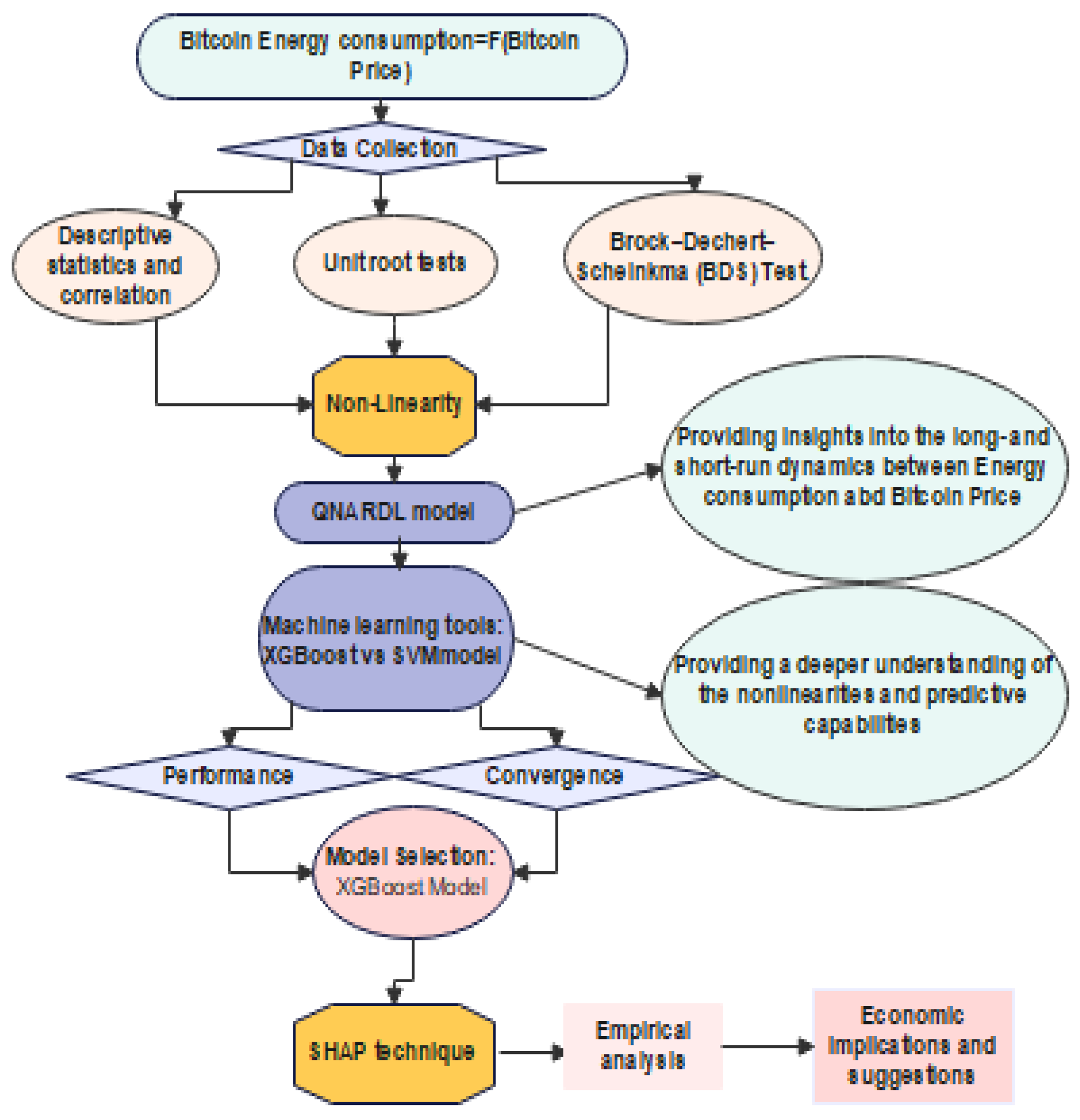
This study will employ a hybrid methodology that combines QNARDL and ML approaches to provide a more thorough examination of the correlation between consumption of energy and Bitcoin prices. While XGBoost and SVM techniques give a deeper grasp of the nonlinearities and prediction capabilities, QNARDL offers insights into the long- and short-term dynamics. Figure 1 shows how the QNARDL and ML models complement each other. First, the QNARDL model is useful for capturing nonlinear interactions between variables. By incorporating ML approaches, notably XGBoost and SVM tools, which excel at capturing complicated nonlinear patterns, the model may better reflect the intricate dynamics of Bitcoin prices and energy use. Second, ML approaches such as XGBoost and SVM models can improve forecasting accuracy by finding patterns and trends that standard econometric models may not detect alone. By combining QNARDL with XGBoost and SVM models, the model can make more accurate forecasts about Bitcoin energy use based on price variations. Furthermore, ML approaches are frequently more resistant to data fluctuations and can adapt to shifting market conditions. By merging QNARDL and ML techniques, the model can better handle the inherent volatility and unpredictability of Bitcoin values and consumption patterns. Third, policymakers and other stakeholders in the energy and cryptocurrency industries can receive improved decision assistance by combining QNARDL with ML approaches. It is possible to make well-informed decisions about infrastructure construction, resource allocation, and policy formulation to reduce the environmental effect of Bitcoin mining by properly forecasting energy usage based on fluctuations in the price of the cryptocurrency.

3.1. Econometrical Methods

To test both the long- and short-run effects of BP on BEC, we first apply the QARDL model proposed by [29]. Compared to the linear model, QARDL allows for asymmetrical localizations in which the parameter relies on the dependent variable locations with their conditional distributions. Besides, the QARDL model simultaneously reports a long-term relationship between variables over the whole quantile scale and short-term dynamics with the conditional distributions of BEC and BP. However, secondly, to test the negative and the positive effect of the BP on the BEC in the given quantiles we apply the nonlinear QARDL which is a transformed form of the QARDL technique. Following [30], we specify the following asymmetric long-run equation of BEC:
l e n c t = α 0 + α 1 l b p t + + α 2 l b p t + ϵ t
where l e n c t refers to the natural logarithm of the Bitcoin energy consumption index, l b p t denotes the Bitcoin price, l b p t + = i = 1 t Δ l b p t + = i = 1 t m a x Δ l b p t , 0 and l b p t = i = 1 t Δ l b p t = i = 1 t m i n Δ l b p t , 0 are the partial sums of both increases and decreases in l b p t · α = α 0 , α 1   a n d   α 2 are the long run parameters to be estimated. Specifically, α 1 and α 2 capture the positive and the negative shocks between Bitcoin price and Bitcoin energy consumption in the long run. Based on information in Equation (1), the quantile ARDL form can be written as follows:
Q Δ l e n c = α 1 ρ l e n c t 1 + α 2 ρ l b p t 1 + + α 3 ρ l b p t 1 + i = 1 p 1 ϕ 1 ρ Δ l e n c t 1 + + i = 1 p 2 ϕ 2 ρ Δ l b p t 1 + + i = 1 p 3 ϕ 3 ρ Δ l b p t 1 + + μ t
where Δ donates the first difference, p = (p1, p2, p3) are the lag orders. α 1 ρ represents the lagged dependent variable parameter. α 2 ρ and α 3 ρ are the parameters of lagged partial sums. β 1 = ϕ 2 ρ α 2 ρ and β 2 = ϕ 3 ρ α 3 ρ represent the long-run impact of the Bitcoin price changes on Bitcoin energy consumption. i = 1 p 2 ϕ 2 ρ and i = 1 p 3 ϕ 3 ρ donate the short positive and effects of the Bitcoin price on Bitcoin energy consumption. μ t is the error term. ρ = 0.1 ; 0.2 ; 0.3 ; 0.4 ; 0.5 ; 0.6 ; 0.7 ; 0.8 ; 0.9 ; 0.95 represents the quantiles. The econometric approach is based on three steps. In the first one, the stationarity of each variable is examined by performing two unit roots tests, namely, the Augmented Dickey-Fuller (ADF) test and the Phillips-Perron test (PP). If the variables have several orders of integration I (0) and I (1), we use quantile regression to predict Equation (2), and the lag duration is chosen in a second phase based on the information criteria AIC or general-to-specific. In the final stage, we perform the Wald test to ensure that the parameters remain constant.

3.2. Machine Learning Methods

Without investigating the extrapolative potential of the BP shocks on BEC, research into the explanatory power of the variables remains restricted. We will employ unusual approaches, mostly machine learning, to accomplish this issue.

3.2.1. Support Vector Machine (SVM or SVR)

The author of [31] created SVM, an organized organization approach that may also be utilized for regression applying the structural risk minimization (SRM) concept for classification and regression. For training data, the SVM approach adopts that, { x i , y i } i = 1 n where x i R L is a vector of L input features, y i R L is the output target, and (n) is the total number of data patterns. The goal of SVM is to create a function f(x) that expects the output value whose variation from the chosen output y i is smaller than the insensible loss parameter ( ε ) for all the training data while being as flat as feasible [32]. In low-dimensional space, the linear regression function is theoretically defined as follows:
f x = w x i + b
where x is the normal to the hyperplane weight vector and b is the hyperplane bias. As seen below, the regression issue is turned into an optimization problem:
minimize 1 2 ω 2 + C i = 1 n ξ i
subjected
to   y i ω x i b ε + ξ i ω x i + b y i ε + ξ i * ξ i , ξ i * 0
ξ i , ξ i * R are the slack variables, while C denotes the punishment coefficient. To solve the optimization issue, the Lagrange multiplier is added, and the regression function has the following form:
f ( x ) = i = 1 l α i α i k x i , x i + b
where α i , α i denotes the Lagrange multiplier, k x i , x i represents the kernel function, and b is computed using the Karush Kuhn-Tucker (KKT) conditions [32].

3.2.2. eXtreme Gradient Boosting (XGBoost) Method

The authors of [33] created XGBoost, an ML approach that may be utilized for regression and classification tasks. This technique has been used in a variety of fields, including healthcare [34] and the metals market [35]. It produces a weak learner at each step and accumulates them in the overall model based on the gradient direction of the loss function. An objective function is regularized to avoid overfitting and to accelerate the studying process. The following is the model output function:
Y ^ i T = k = 1 T f k x i = y ^ i T 1 + f T x i
If y ^ i T 1 denotes the generated tree, f T x i embodies the freshly constructed tree model, and T presents the entire number of tree models. Furthermore, ref. [36] said that XGBoost is resilient in terms of modeling nonlinear correlations between the variables. It is extremely capable of classification. As a result, numerous academics have said that ML is an effective approach for predicting time-series data. Nevertheless, classical econometrics does not offer interpretable findings. The authors of [37] presented a Shapley additive clarification approach (SHAP) to grasp the estimation of ML methods based on game theory pioneered by [38] to enhance the performance of XGBoost. By assessing the influence of each feature on prediction, we may use the SHAP technique to expound the forecast of a given input (X). The main assumption of SHAP is to run the Shapley values for all features of the sample to be understood, where each Shapley value computes the impact that the associated feature has on the prediction. Furthermore, ML models typically have many features, each of which is a discrete or continuous variable, making it computationally very difficult to compute the Shapley values for each occurrence of each feature, and the SHAP procedure is better suited to splitting with the concern at hand.
The estimated Shapley value is calculated as follows:
ϕ ^ j = 1 K k = 1 K g ^ x + j m g ^ x j m
where g ^ x + j m is the prediction for x, but with a random number of feature values.
We utilize two metrics to evaluate the prediction performance of the various models, the RMSE and R2, which are obtained as follows:
R o o t   M e a n   S q u a r e   E r r o r   ( R M S E )   = 1 N V t = 1 N v y t y ^ t 2
c o e f f i c i e n t   o f   d e t e r m i n a t i o n   ( R 2 )   = 1 t = 1 N ( y t y ^ t ) 2 t = 1 N ( y t y t ¯ ) 2
M e a n   s q u a r e d   e r r o r   ( M S E )   = 1 N V t = 1 N v ( y t y ^ t ) 2
where y ^ t is the predicted BEC, y t is the t th current BEC, y t ¯ represents the mean BEC, and N v represents the number of observations served throughout the forecasting validation phase.

4. Model Estimation and Results

4.1. Data Analysis

In this study, the variables are the estimated energy consumption (LENC) for mining Bitcoin daily in Terawatt–Hours (TWh) and USD market prices of Bitcoin (LBP) collected from https://digiconomist.net/ and www.bitcoinity.org/, accessed on 1 January 2023, respectively. All variables are expressed in natural logarithm which can reduce both the heteroscedasticity intensity and volatility excess. The spanning period is from 1 July 2010 to 1 December 2022, while the frequency of the observations is monthly. In addition to this, several symbols and notations are used in our study; they are included in Table 1. Table 2 donates the descriptive statistics. The Jarque–Bera test declines the null of normality for BEC and BP, hence, the quantile regression is appropriate. Moreover, our variables seem to move together in the long run given the high correlation result of 0.7799. Figure 2 illustrates the dynamic pattern of BP and the BEC index since 2010.
Figure 3 shows a substantial rise in both BP and energy consumption from 2018. Moreover, there was an intersection between the two curves in the sixth month of 2018, showing the acceleration of energy consumption after a clear and continuous rise in the price of Bitcoin, which went from USD 8000 in January 2017 to USD 20,000 in December of the same year. Table 3 displays the results of the unit roots tests from which it can be recorded that the default hypothesis of the unit root is accepted for LENC at 5% of significance level and rejected for LBP. Otherwise, in the first difference, all unit root tests decline the default hypothesis at the 1% significance level.
To detect the nonlinear link between BEC and BP, we apply the nonlinearity Brock–Dechert–Scheinkma test proposed by [12]. The authors indicated that when the null hypothesis is rejected, chaotic and nonlinear dependencies are present in the time series. Results from Table 4 indicate that the null hypothesis of the BDS test was denied at a 1% level of significance under different dimensions m = (2, 3, 4 and 6) for all series. Like [39], our findings showed the rejection of the hypothesis that the series comes from the white noise i.i.d processes. Also, ref. [12] showed that the behavior of the two series is chaotic and non-linear when using the BDS test. This means that the nonlinear model is more appropriate to examine the relationship between BEC and BP than the linear model. Regarding co-integration, both time series unit root tests confirm that all variables are in a mixed order of integration (I (0), I (1)), and no I (2) variables are involved. Table 5 reports the results of the co-integration F-statistics at a 5% level of significance. The calculated F-statistic is greater than the upper bound for all the quantiles except ρ = 0.2 and ρ = 0.3, which confirm co-integration among variables.

4.2. Empirical Results and Discussions

4.2.1. Econometrical Results

The findings from the QNARDL estimation are stated in Table 5. R-4.4.0 software is used to achieve all estimations. The outputs indicate that in the short run, BP is positively related to the BEC overall quantiles. This means that any increase in BP leads to a rise in energy consumption. In addition, in the long run, results show that BP increases energy consumption only in the first and the last quantiles. Overall, the higher the value of Bitcoin, the more attractive the activity. Indeed, Bitcoin is based on blockchain technology which is a decentralized digital ledger that records all trade made with cryptocurrency. To guarantee the security, integrity, and decentralization of this ledger, cryptocurrencies use a process called “proof of work” (PoW) to validate transactions and add new blocks to the chain. The proof-of-work process involves miners solving complex mathematical problems. To solve these problems, miners must perform complex, energy-intensive calculations, using the computing power of their computers. The first miner to resolve the problem correctly is rewarded with new cryptocurrency units and the right to add a new block to the blockchain. However, due to the growing complexity of the mathematical problems to be solved and the competition between miners, the computing power required to mine new units of cryptocurrency has increased considerably over time. This has led to a significant expansion in the energy consumption associated with mining cryptocurrencies like Bitcoin. Moreover, Wald test results exhibited in Table 6 indicate that the null hypothesis of symmetry is rejected in both the short and long term. This implies that the connection between the BEC and the BP is asymmetric.
From the QNARDL results mentioned in Table 7, we can observe that in the short-run, coefficients of lbp+ and lbp are positive and significant at a 1% significance level in the high quantiles. Hence, a one percent increase in BP increases BEC by 6% in the ρ95 quantiles. Further, estimation results report that a one percent decrease in BP raises energy consumption by 12% in the ρ9 quantiles. Our results are like the findings of [27] which showed that the Bitcoin market and energy consumption presented a strong risk.
Thus, the Bitcoin money market value continues to increase due to speculation; therefore, the more its money price increases, the more its electricity consumption soars. Indeed, this cryptocurrency is based on a decentralized system. This means that each transaction made must go through different computers in the large cryptocurrency network. Bitcoin needs great computing power to do this. Moreover, total computing power is suitable for the reward at stake. In the short term, therefore, the hash rate is correlated to the price of Bitcoin. When the price goes up, computing power gradually increases. When it goes down, the opposite happens: some miners give up and stop their activity because they are no longer profitable. Thus, the monstrous consumption of electricity is linked to the speculation behind Bitcoin: Bitcoin is for the moment very overvalued compared to its real utility.
Otherwise, the asymmetric long-term connection between BEC and BP remains negatively significant for the ρ95 quantiles. Results indicate that a one percent increase in BP decreases BEC by 42%. However, a one percent decrease in lbp decreases LENC by almost 88%. Thus, in the longer term, the reward will also be influenced by the number of Bitcoins issued by the protocol: it decreases regularly. This drop in reward will also influence mining: in this way, even if the price peaks, it is very likely that the energy expended stabilizes over time, relying more and more on the fees paid by users. Table 8 summarizes the Wald tests of the QNARDL model. Findings indicate that the null hypothesis is accepted for the long-run parameters and rejected for the short-run parameters. Acceptance of the null hypothesis indicates the constancy of the long-run parameters between the increase and the decrease of the BP across the quantiles. Hence, the link between BP and BEC is linear in the long term. However, in the short run, the Bitcoin price–energy consumption nexus is nonlinear.

4.2.2. Machine Learning Results

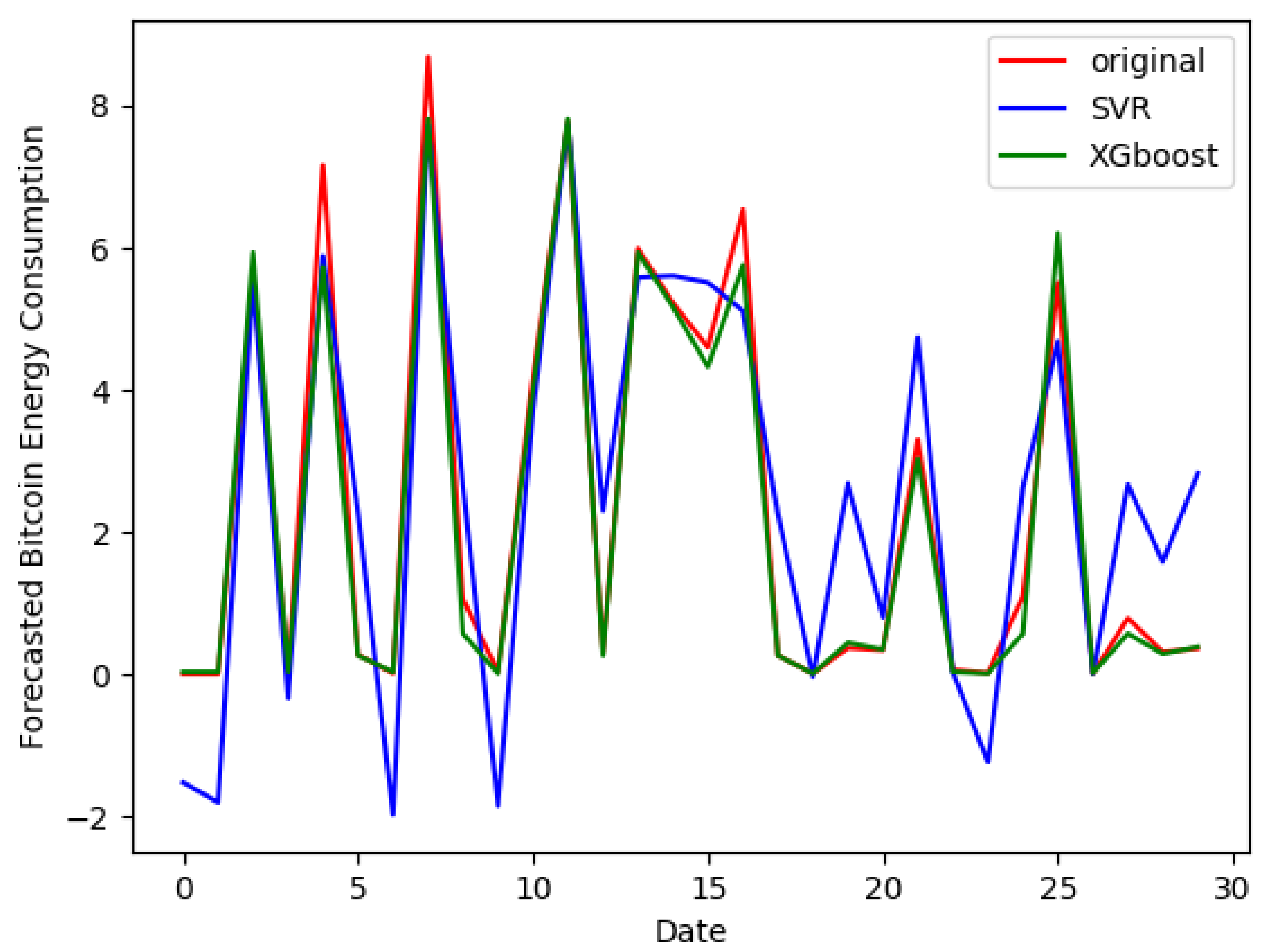
Now, we discuss the findings of the machine learning tools. We investigate the simultaneous effect of positive and negative shocks of BP on the BEC. This enables a deeper comprehension of how several shocks interact to affect BEC. Figure 3 plots the forecasted and observed values of BEC by comparing the SVR model against the XGBoost model on a validation sample. The plot indicates that the curve of the predicted series generated by the XGBoost model (green curve) closely aligns with the actual values (red curves), demonstrating its effectiveness in capturing the underlying patterns in BEC data. We highlight that the curve generated by the SVR model (blue curve) adopts a very different behavior compared to the curve of the actual values of BEC. This suggests that the XGBoost model outperforms the SVR model in terms of BEC forecasting accuracy. In addition, we report the ability of the XGBoost model as a machine learning tool to determine a good forecast of BEC, better than the SVR model. To summarize, our study shows that the XGBoost model outperforms the SVR model in terms of BEC prediction. This emphasizes how crucial it is to use cutting-edge machine learning techniques to raise the precision and dependability of energy consumption predictions within the Bitcoin ecosystem.
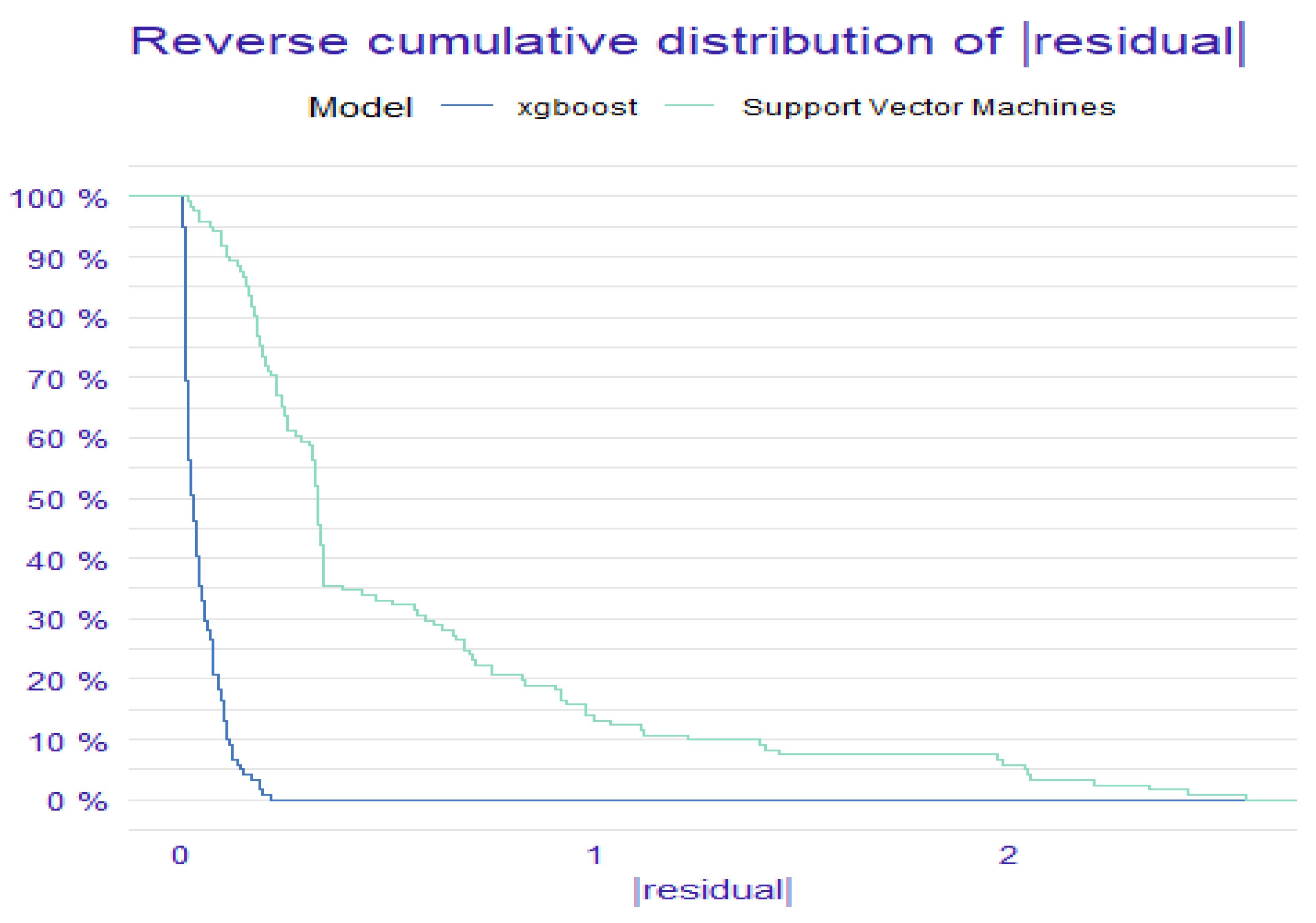
In terms of performance, the findings in Table 9 confirm the outperformance and dominance of the XGBoost model when compared to the SVR model. Empirical evidence exhibits that the assessments of performance metrics generated by the XGBoost model (RMSE = 0.72; MAE = 0.52) are smaller compared to those of the SVR model. In addition, the value of R2 of the XGBoost model is higher than that generated by the SVR model. Furthermore, Figure 4 plots the convergence of ML tools. It depicts the behavior of the “RMSE” cost function. We find that the XGBoost model achieves good root mean square error (RMSE) convergence compared to the SVR model. This means that the XGBoost model allows the cost function to quickly converge to the optimal solution. We also see that the RMSE convergence is more pronounced in the case of the XGBoost model than in the SVR model. This implies that, in terms of convergence, the XGBoost model is more efficient than the SVM model. We complement the analysis by focusing on the features of the XGBoost forecasting tool. The SVR model is discarded from the feature assessment since it is less effective and good compared to the XGBoost model.
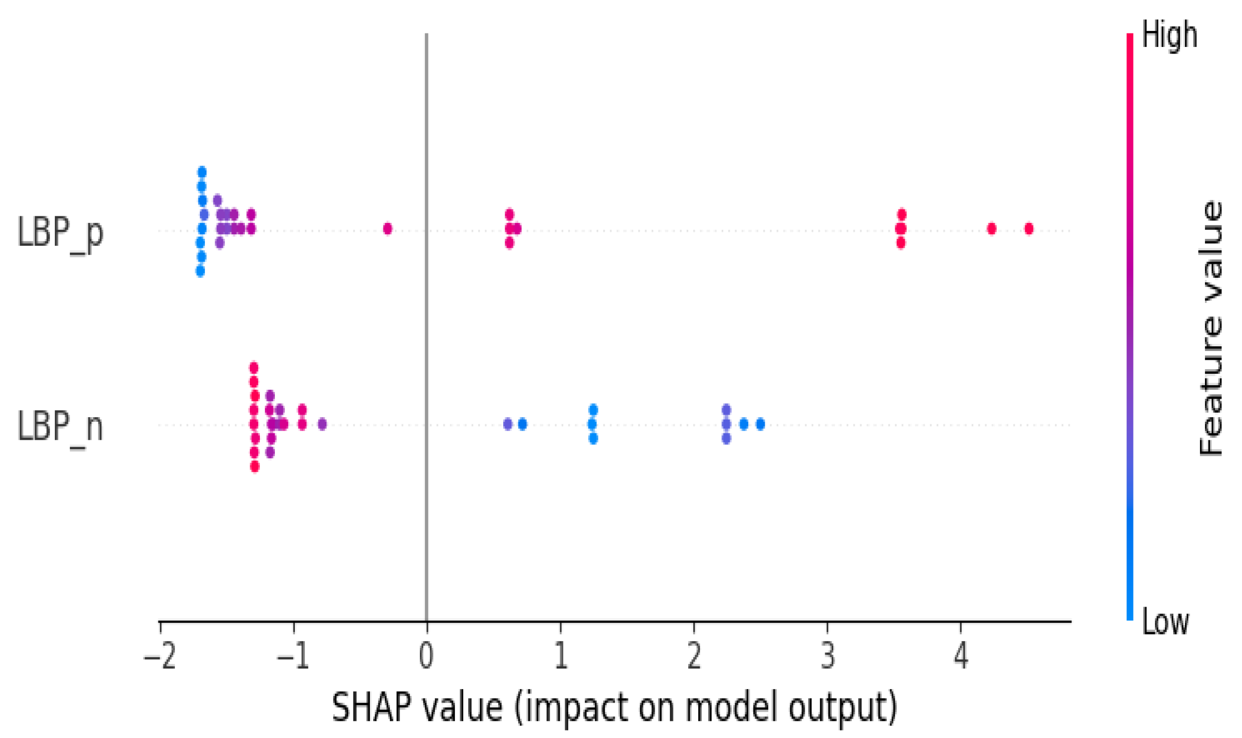
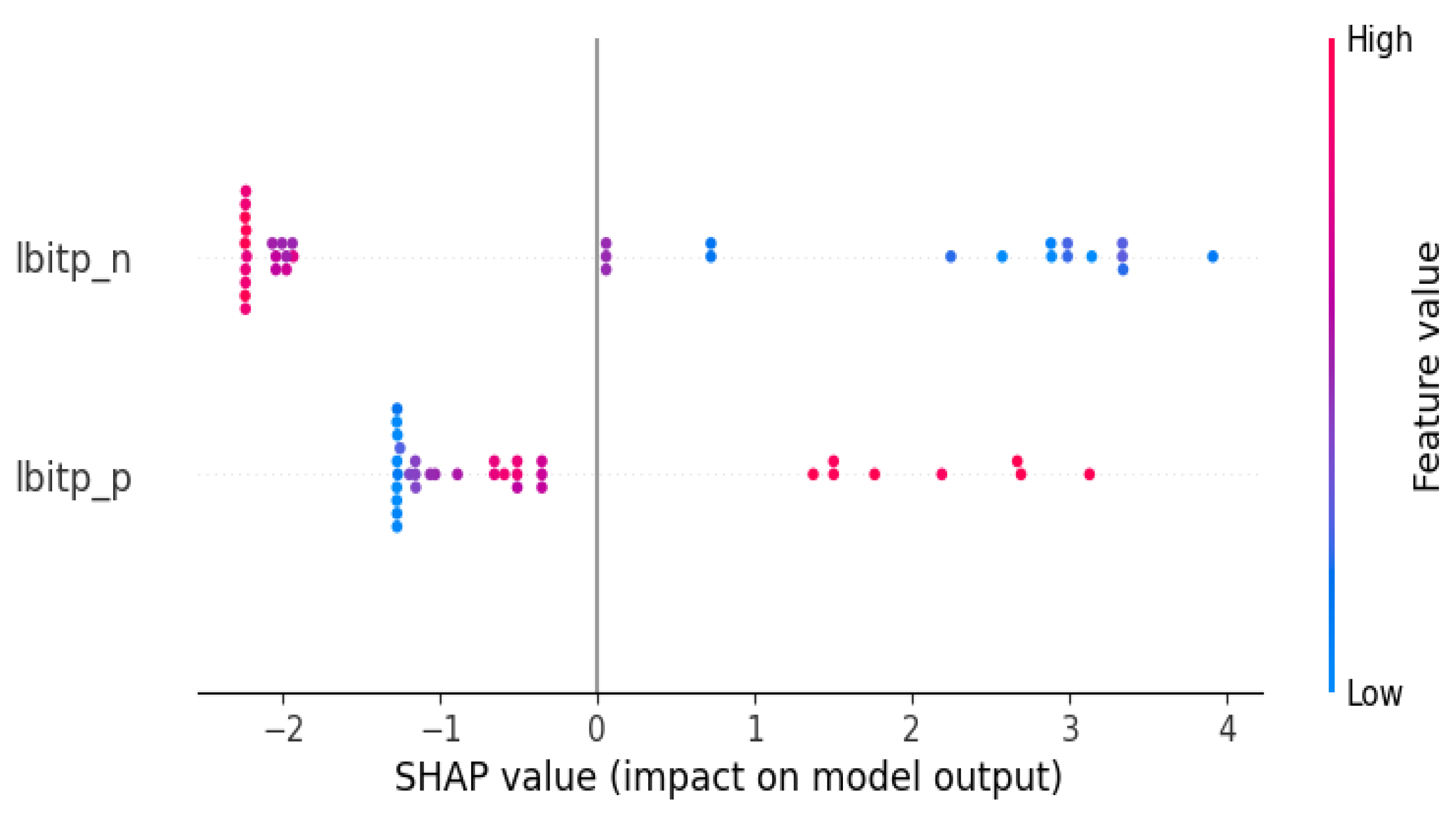
The above-mentioned analysis indicates that the performance metrics and convergence of the “RMSE” cost function show that XGBoost appears dominant over the SVR model in terms of convergence and performance, supporting the quality of the prediction when using the XGBoost tool. However, the analysis is not able to show the contribution or the importance of each feature on the prediction of the model. In other words, the previous analysis does not show the participation of positive and negative shocks of BP for the forecasting of BEC. To complement this, the next step is to determine the significance or contribution of the features to the overall dataset. The bee swarm plot is thus adopted as an option. Regarding this method, the features are likewise organized by their influence on prediction. Also, we can observe how higher and lower feature values affect the prediction. The results of this method are plotted in Figure 5. We see that the positive shock to the BP has a positive impact when its values are high and a negative contribution when its values are low. However, high levels of positive shock to BP have a positive contribution to the forecast, and low values have a negative impact. This indicates that the positive shock to the BP dominates the negative shock to the BP in terms of contribution to the forecast of BEC. In addition to this, we illustrate that positive shock to the BP is an important source for BEC forecasting. By illustrating the importance of positive shocks to the Bitcoin price as a key source for forecasting energy consumption, our analysis provides valuable insights for understanding the dynamics between Bitcoin price movements and energy usage in the network. It highlights the need to consider not only the direction but also the magnitude of price shocks when predicting energy consumption in the Bitcoin ecosystem.

5. Robustness Analysis

The entire purpose of this section is to evaluate how reliable our preliminary findings are. Our contribution to this stage is to consider the most recent market data using the same machine-learning methods. Due to the extreme volatility that typifies the cryptocurrency market and the shift in data speed within it, these data have been integrated into the study. To reflect the current situation more correctly, our analysis may take into account upgrading the data to the most recent time, given that it aligns with several geopolitical occurrences, including the conflict between Russia and Ukraine. Accordingly, we re-examine the predictive power of positive and negative shocks of Bitcoin prices for Bitcoin energy consumption by applying the Support Vector Machine (SVM) and eXtreme Gradient Boosting (XGBoost) on monthly data that span from 1 July 2010 to 1 May 2024.
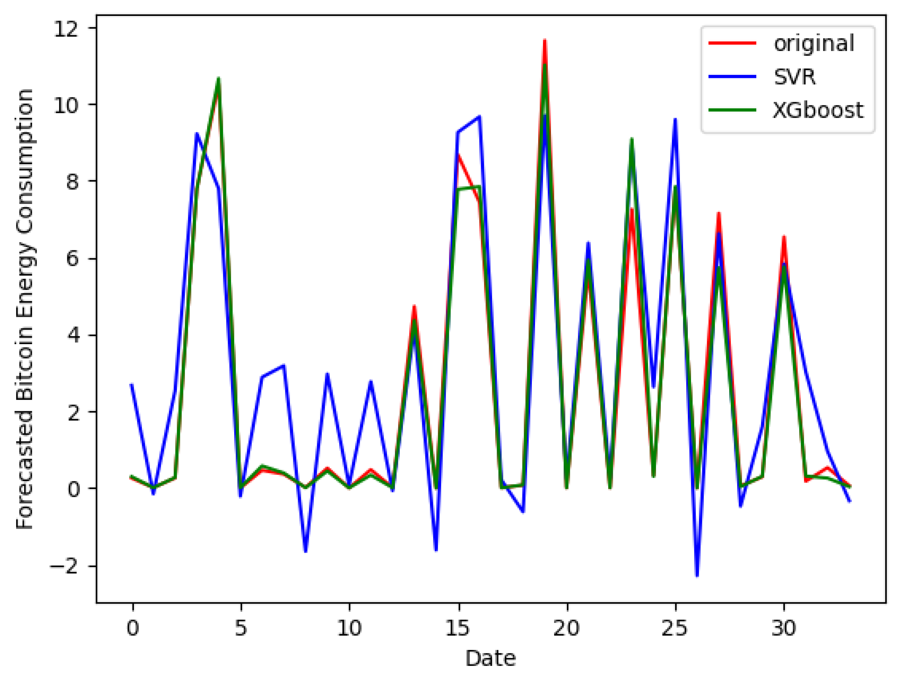
Significant results from the robustness analysis were obtained. First, Figure 6 compares the SVR model with the XGBoost model on a validation sample, plotting the predicted and observed values of BEC. We demonstrate that almost aligned with the red curves (actual values) is the predicted series curve generated by the XGBoost model. It should be noted, however, that the SVR model’s generated curve behaves much differently from the curve representing actual BEC values. This suggests that when it comes to BEC predicting, the XGBoost model outperforms the SVR model. Furthermore, we find that the XGBoost model outperforms the SVR model as a machine learning method in determining an accurate BEC forecast. Table 10’s performance results validate the superiority and domination of the XGBoost model over the SVR model. Based on empirical data, the performance metrics evaluated by the XGBoost model (RMSE = 0.00057; MSE = 0.000033) are lower when compared to the SVR model. Furthermore, the XGBoost model’s R2 value is greater than that of the SVR model. Just like in the primary study, we enrich the analysis by focusing on the characteristics of the XGBoost forecasting tool. The SVR model is excluded from the feature evaluation since it is less effective and excellent than the XGBoost model. However, we see that the performance metrics generated by XGBoost in the robustness portion are significantly improved when compared to the values generated in the main section. This suggests that the XGBoost tool is more successful at predicting when the database will grow in volatile tendency.
The importance or contribution of every feature to the entire dataset must next be ascertained. It is decided to go with the bee swarm plot as a possibility. Concerning this methodology, the features are also arranged according to their impact on forecasting. Furthermore, we can see how higher and lower feature values influence the prediction [40,41]. The outcomes of this approach are shown in Figure 7. The negative shock to BP contributes positively to prediction of BEC when its levels are low and negatively when they are high. This implies that there is a positive influence on BEC forecasts during periods of notable drops in Bitcoin value, which may indicate more energy use during market downturns.
However, large levels of positive shock to BP contribute positively to the forecasting, whereas low levels have a negative influence in forecasting the BEC. It may be inferred from this that notable spikes in Bitcoin values have a favorable impact on BEC prediction, possibly due to increased energy-intensive mining activities during value booms. This suggests that the negative shock to the BP outweighs the positive shock in terms of contribution to the BEC projection. In addition, we show that negative shocks to the BP are a major source of BEC forecasting, suggesting that periods of price decline significantly influence energy consumption patterns. In comparison to the main research, the impact of both positive and negative shocks to BP for BEC projection is more pronounced when taking the most recent period into account. This suggests that energy consumption estimates are more sensitive to recent fluctuations in Bitcoin values, underscoring the need for real-time data in predictive modeling.

6. Conclusions and Implications

This study used the QNARDL model to investigate the asymmetric long- and short-term relationships between BEC and BP. The results show that the relationship between BEC and BP is asymmetric. Furthermore, our findings demonstrate that fluctuations in BP have important short- and long-term effects on BEC. As a result, every increase in the BP raises energy usage in the near term. In addition, a short-term decline in Bitcoin value increases energy usage. However, rising BP in the long term decreases energy consumption. Otherwise, any drop in the BP decreases energy consumption in the long run. When considering machine learning tools, results showed that, in terms of its contribution to the BEC prediction, the positive shock to the price of Bitcoin outweighs the negative shock. Furthermore, we show that a positive shock to the price of Bitcoin serves as a valuable source of information for BEC predictions. These results are in line with the QNARDL model. In addition to this, the use of the XGBoost machine learning tool provides evidence that the positive shock to the BP outweighs the negative shock in terms of contributing to BEC’s prediction. Also, we show that a positive shock to the BP is a major source of BEC forecasts.
Our results suggest many implications. First, the identification of the asymmetric impacts of Bitcoin prices on energy usage is one of the main practical consequences of our research. Through a knowledge of how fluctuations in Bitcoin values affect energy use, interested parties may design focused interventions to maximize energy efficiency and minimize use when the market is volatile. Second, our study also emphasizes the necessity of dynamic energy management plans that can adjust energy usage in reaction to changes in Bitcoin pricing. Mining companies may improve energy use to reduce their environmental impact and increase profitability by utilizing real-time data and predictive analytics. Third, the environmental effects of Bitcoin energy consumption may be lessened by promoting the use of renewable energy sources for cryptocurrency mining. Subsidies, tax breaks, and partnerships with renewable energy suppliers can be used by stakeholders to encourage miners to switch to renewable energy sources. Fourth, to encourage environmentally sustainable practices in the Bitcoin business, regulators can also impose regulatory measures like energy usage limitations, carbon pricing systems, or emissions trading programs. Miners might be encouraged to emphasize energy efficiency and lessen their carbon impact by authorities establishing clear criteria and incentives. Five, mining activities could be expanded to cover additional cryptocurrencies or blockchain projects with varying energy needs and pricing dynamics. Utilizing possibilities in other markets can help disperse risk and lessen the impact of Bitcoin price shocks on energy use. Finally, demand response initiatives that encourage energy users—including Bitcoin miners—to modify their electricity usage in reaction to market fluctuations could be implemented. In addition to possibly earning prizes or incentives, miners may help maintain grid stability by voluntarily consuming less energy during periods of high demand or low energy costs. Implementing these measures allows participants in the cryptocurrency ecosystem to better control the effects of Bitcoin price shocks on energy usage while also boosting sustainability, efficiency, and resilience in mining operations.
This article has some shortcomings, even though it offers numerous significant findings and policy implications. The study of Bitcoin’s energy consumption only reflects part of the problem. Other cryptocurrencies are in even greater demand than Bitcoin, such as Ethereum, and also consume energy and need to be explored. In addition, the world of machine learning offers several interesting methods, mainly those based on deep learning, which we plan to explore in future research projects. In particular, Multi-agent deep reinforcement learning (MARDL) extends the principle of deep learning to environments where several agents interact [42,43].

Author Contributions

Conceptualization, K.T., T.Z. and S.B.; Data curation, M.T.; Formal analysis, K.T. and M.T.; Funding acquisition, K.T.; Investigation, T.Z. and B.H.; Methodology, T.Z. and B.H.; Project administration, K.T.; Software, T.Z.; Supervision, B.H.; Validation, K.T.; Visualization, S.B.; Writing—original draft, T.Z. and S.B.; Writing—review & editing, K.T. and T.Z. All authors have read and agreed to the published version of the manuscript.

Funding

This research has been funded by Scientific Research Deanship at the University of Ha’il–Saudi Arabia through project number RG-21 156.

Data Availability Statement

Data are contained within the article.

Conflicts of Interest

The authors declare no conflicts of interest.

References

  1. Mudassir, M.; Bennbaia, S.; Unal, D.; Hammoudeh, M. Time-series forecasting of Bitcoin prices using high-dimensional features: A machine learning approach. Neural Comput. Appl. 2020, 1–5. [Google Scholar] [CrossRef]
  2. Jana, R.K.; Ghosh, I.; Wallin, M.W. Taming energy and electronic waste generation in Bitcoin mining: Insights from Facebook prophet and deep neural network. Technol. Forecast. Soc. Chang. 2022, 178, 121584. [Google Scholar] [CrossRef]
  3. Atsalakis, G.S.; Atsalaki, I.G.; Pasiouras, F.; Zopounidis, C. Bitcoin price forecasting with neuro-fuzzy techniques. Eur. J. Oper. Res. 2019, 276, 770–780. [Google Scholar] [CrossRef]
  4. Chen, C.; Liu, L.; Zhao, N. Fear sentiment, uncertainty, and Bitcoin price dynamics: The case of COVID-19. In Research on Pandemics; Routledge: London, UK, 2021; pp. 166–177. [Google Scholar]
  5. Tissaoui, K.; Zaghdoudi, T.; issa Alfreahat, K. Can intraday public information explain Bitcoin Returns and Volatility? A PGARCH-Based Approach. Econ. Bull. 2020, 40, 2085–2092. [Google Scholar]
  6. Bouri, E.; Gupta, R.; Tiwari, A.K.; Roubaud, D. Does Bitcoin hedge global uncertainty? Evidence from wavelet-based quantile-in-quantile regressions. Fin. Res. Lett. 2017, 23, 87–95. [Google Scholar] [CrossRef]
  7. Katsiampa, P. Volatility estimation for Bitcoin: A comparison of GARCH models. Econ. Lett. 2017, 158, 3–6. [Google Scholar] [CrossRef]
  8. Cheah, E.T.; Fry, J. Speculative bubbles in Bitcoin markets? An empirical investigation into the fundamental value of Bitcoin. Econ. Lett. 2015, 130, 32–36. [Google Scholar] [CrossRef]
  9. Tiwari, A.K.; Jana, R.K.; Das, D.; Roubaud, D. Informational efficiency of Bitcoin—An extension. Econ. Lett. 2018, 163, 106–109. [Google Scholar] [CrossRef]
  10. Baur, D.G.; Dimpfl, T. Price discovery in Bitcoin spot or futures? J. Futures Mark. 2019, 39, 803–817. [Google Scholar] [CrossRef]
  11. Yao, W.; Xu, K.; Li, Q. Exploring the influence of news articles on Bitcoin price with machine learning. In Proceedings of the 2019 IEEE Symposium on Computers and Communications (ISCC) 2019, Barcelona, Spain, 29 June–3 July 2019; pp. 1–6. [Google Scholar]
  12. Maiti, M. Dynamics of Bitcoin prices and energy consumption. Chaos Solitons Fractals X 2022, 9, 100086. [Google Scholar] [CrossRef]
  13. Das, D.; Dutta, A. Bitcoin’s energy consumption: Is it the Achilles heel to miner’s revenue? Econ. Lett. 2020, 186, 108530. [Google Scholar] [CrossRef]
  14. Küfeoglu, S.; Özkuran, M. Energy Consumption of Bitcoin Mining; Faculty of Economics, University of Cambridge: Cambridge, UK, 2019. [Google Scholar]
  15. Li, J.; Li, N.; Peng, J.; Cui, H.; Wu, Z. Energy consumption of cryptocurrency mining: A study of electricity consumption in mining cryptocurrencies. Energy 2019, 168, 160–168. [Google Scholar] [CrossRef]
  16. Greenwood-Nimmo, M.; Kim, T.H.; Shin, Y.; Van Treeck, T. Fundamental Asymmetries in US Monetary Policymaking: Evidence from a Nonlinear Autoregressive Distributed Lag Quantile Regression Model; Leeds University Business School: Leeds, UK, 2011. [Google Scholar]
  17. Diks, C.; Panchenko, V. A new statistic and practical guidelines for nonparametric Granger causality testing. J. Econ. Dyn. Control. 2006, 30, 1647–1669. [Google Scholar] [CrossRef]
  18. Boz, E.; Mendoza, E.G. Financial innovation, the discovery of risk, and the US credit crisis. J. Monet. Econ. 2014, 62, 1–22. [Google Scholar] [CrossRef]
  19. Nakamoto, S. Bitcoin P2P e-Cash Paper. The Cryptography Mailing List; Nakamoto Institute: Austin, TX, USA, 2008. [Google Scholar]
  20. Sarkodie, S.A.; Ahmed, M.Y.; Leirvik, T. Trade volume affects Bitcoin energy consumption and carbon footprint. Fin. Res. Lett. 2022, 48, 102977. [Google Scholar] [CrossRef]
  21. Oprea, S.V.; Georgescu, I.A.; Bâra, A. Is Bitcoin ready to be a widespread payment method? Using price volatility and setting strategies for merchants. Electron. Commer. Res. 2024, 1–39. [Google Scholar] [CrossRef]
  22. Bâra, A.; Oprea, S.V.; Panait, M. Insights into Bitcoin and energy nexus. A Bitcoin price prediction in bull and bear markets using a complex meta model and SQL analytical functions. Appl. Intell. 2024, 1–29. [Google Scholar] [CrossRef]
  23. Bâra, A.; Oprea, S.V. An ensemble learning method for Bitcoin price prediction based on volatility indicators and trend. Eng. Appl. Artif. Intell. 2024, 133, 107991. [Google Scholar] [CrossRef]
  24. Chitkasame, T.; Rakpho, P.; Khiewngamdee, C. Analyzing structural change and causality between energy consumption and bitcoin’s activity. Energy Rep. 2022, 8, 736–743. [Google Scholar] [CrossRef]
  25. Hong, H.; Zhang, C. Bitcoin trading, economic growth, energy use, and CO2 emissions: An advanced panel study of emerging market economies. Int. Rev. Econ. Finance 2023, 87, 519–531. [Google Scholar] [CrossRef]
  26. Mohsin, M.; Naseem, S.; Zia-ur-Rehman, M.; Baig, S.A.; Salamat, S. The crypto-trade volume, GDP, energy use, and environmental degradation sustainability: An analysis of the top 20 crypto-trader countries. Int. J. Financ. Econ. 2023, 28, 651–667. [Google Scholar] [CrossRef]
  27. Yan, L.; Mirza, N.; Umar, M. The cryptocurrency uncertainties and investment transitions: Evidence from high and low carbon energy funds in China. Technol. Forecast. Soc. Chang. 2022, 175, 121326. [Google Scholar] [CrossRef]
  28. Sarker, P.K.; Lau, C.K.; Pradhan, A.K. Asymmetric effects of climate policy uncertainty and energy prices on Bitcoin prices. Innov. Green Dev. 2023, 2, 100048. [Google Scholar] [CrossRef]
  29. Cho, J.S.; Kim, T.H.; Shin, Y. Quantile cointegration in the autoregressive distributed-lag modeling framework. J. Econ. 2015, 188, 281–300. [Google Scholar] [CrossRef]
  30. Shin, Y.; Yu, B.; Greenwood-Nimmo, M. Modelling asymmetric cointegration and dynamic multipliers in a nonlinear ARDL framework. In Festschrift in Honor of Peter Schmidt: Econometric Methods and Applications; Springer: New York, NY, USA, 2014; pp. 281–314. [Google Scholar]
  31. Vapnik, V.N. The Support Vector Method. In Proceedings of the International Conference on Artificial Neural Networks, Lausanne, Switzerland, 12 June 1997; Springer: Berlin/Heidelberg, Germany, 1997; pp. 261–271. [Google Scholar]
  32. Smola, A.J.; Schölkopf, B. A tutorial on support vector regression. Stat. Comput. 2004, 14, 199–222. [Google Scholar] [CrossRef]
  33. Ostrowski, K.; Birman, K. Extensible web services architecture for notification in large-scale systems. In Proceedings of the 2006 IEEE International Conference on Web Services (ICWS’06), Chicago, IL, USA, 18–22 September 2006; pp. 383–392. [Google Scholar]
  34. Singh, N.; Singh, P.; Bhagat, D. A rule extraction approach from support vector machines for diagnosing hypertension among diabetics. Expert Syst. Appl. 2019, 130, 188–205. [Google Scholar] [CrossRef]
  35. Jabeur, S.B.; Khalfaoui, R.; Arfi, W.B. The effect of green energy, global environmental indexes, and stock markets in predicting oil price crashes: Evidence from explainable machine learning. J. Environ. Manag. 2021, 298, 113511. [Google Scholar] [CrossRef] [PubMed]
  36. Ma, B.; Meng, F.; Yan, G.; Yan, H.; Chai, B.; Song, F. Diagnostic classification of cancers using extreme gradient boosting algorithm and multiomics data. Comput. Biol. Med. 2020, 121, 103761. [Google Scholar] [CrossRef] [PubMed]
  37. Lundberg, S.M.; Lee, S.I. A unified approach to interpreting model predictions. In Proceedings of the Advances in Neural Information Processing Systems, Long Beach, CA, USA, 4–9 December 2017; pp. 4765–4774. [Google Scholar]
  38. Shapley, L.S. A value for n-person games. In Contributions to the Theory of Games; Princeton University Press: Princeton, NJ, USA, 1953; pp. 307–317. [Google Scholar]
  39. Günay, S. Chaotic structure of the BRIC countries and Turkey’s stock market. Int. J. Econ. Financ. Issues 2015, 5, 515–522. [Google Scholar]
  40. Zaghdoudi, T.; Tissaoui, K.; Hakimi, A.; Ben Amor, L. Dirty versus renewable energy consumption in China: A comparative analysis between conventional and non-conventional approaches. Ann. Oper. Res. 2024, 334, 601–622. [Google Scholar] [CrossRef]
  41. Tissaoui, K.; Zaghdoudi, T.; Hakimi, A.; Nsaibi, M. Do gas price and uncertainty indices forecast crude oil prices? Fresh evidence through XGBoost modeling. Comput. Econ. 2023, 62, 663–687. [Google Scholar] [CrossRef] [PubMed]
  42. Yang, L.; Li, X.; Sun, M.; Sun, C. Hybrid policy-based reinforcement learning of adaptive energy management for the Energy transmission-constrained island group. IEEE Trans. Ind. Inform. 2023, 19, 10751–10762. [Google Scholar] [CrossRef]
  43. Yan, Z.; Xu, Y. A multi-agent deep reinforcement learning method for cooperative load frequency control of a multi-area power system. IEEE Trans. Power Syst. 2020, 35, 4599–4608. [Google Scholar] [CrossRef]
Figure 1. Integration of QARDL and ML: Process Flow Diagram.
Energies 17 02810 g001
Figure 2. Bitcoin price and Bitcoin energy consumption index trends.
Energies 17 02810 g002
Figure 3. Plot of forecasted Bitcoin energy consumption.
Energies 17 02810 g003
Figure 4. Plot of residual convergence.
Energies 17 02810 g004
Figure 5. Plot of feature importance.
Energies 17 02810 g005
Figure 6. Plot of BEC forecast when considering recent market data.
Energies 17 02810 g006
Figure 7. Plot of feature importance when considering recent market data.
Energies 17 02810 g007
Table 1. List of Notations.
SymbolMeaning
QNARDLQuantile nonlinear autoregressive distributed lags model
XGBoosteXtreme Gradient Boosting
SVM or SVRSupport Vector Machine
SHAPShapley additive clarification approach
MLMachine learning
BECBitcoin energy consumption
BPBitcoin price
LENCThe logarithm of Bitcoin Energy Consumption
LBPThe logarithm of Bitcoin Price
ADFAugmented Dickey-Fuller test
PPPhillips–Perron test
RMSERoot Mean Square Error
MSEMean squared error
R2Coefficient of determination
Notes: The symbols used in this table are consistent with their representation throughout the manuscript.
Table 2. Descriptive statistics and correlation.
LBPLENC
Mean3.73331.6058
Maximum4.28991.864045
Minimum2.97190.968053
Std. Dev.0.28970.294868
Jarque-Bera133.5838160.7121
Probability0.0000 ***0.0000 ***
Correlation0.7799
Observations1024
Notes: *** donates the statistical significance at 1%.
Table 3. Unit root tests.
ADFPP
VariablesAt LevelFirst DifferenceAt LevelFirst Difference
LENC−3.322298 **−9.623965 ***−2.654289 *−23.48186 ***
LBP−2.527610−31.78289 ***−2.509067−31.82790 ***
Notes: ***, **, * donate the statistical significance at 1%, 5%, and 10%, respectively.
Table 4. Brock–Dechert–Scheinkma (BDS) Test.
DimensionBDS-Stat
LBPLENC
20.1986 ***0.2093 ***
30.3380 ***0.3557 ***
40.4350 ***0.4579 ***
50.5019 ***0.5292 ***
60.5477 ***0.5789 ***
Notes: *** donates statistical significance at 1%.
Table 5. QARDL estimation results.
ρ0.10.20.30.40.50.70.80.90.95
Short-Run
Cons−0.036 ***−0.0270 *−0.0262−0.0300 *−0.0359 *−0.0274−0.0204−0.00880.0358
LENC_10.7980 ***0.9107 ***0.9569 ***0.9790 ***1.0079 ***1.0491 ***1.0618 ***1.1039 ***1.1445 ***
L.LBP0.0138 ***0.0112 *0.0135 *0.0214 ***0.0265 ***0.0237 **0.02610.0271 *0.0199
D.LBP0.01150.04590.0330−0.0039−0.0283−0.03130.05620.0758−0.0322
L.D.LBP0.1065 ***0.0794 *0.1089 **0.1587 ***0.2366 ***0.3237 ***0.3652 ***0.3444 ***0.3488 ***
Long-Run
L.LBP0.0683 *0.12510.31281.0189−3.3753−0.4832−0.4214−0.2605 *−0.1380 *
D.LBP0.05710.5136 ***0.7656 *−0.18773.60930.6379−0.909 ***−0.729 ***0.222 ***
L.D.LBP0.5269 ***0.8896 ***2.5293 ***7.5441 ***−30.13 ***−6.588 ***−5.905 ***−3.313 ***−2.413 ***
Notes: ***, **, * donate the statistical significance at 1%, 5% and 10%, respectively.
Table 6. Wald Test for the constancy of parameters (QARDL).
W s r ϕ W l r β W s r γ
LENC_1L.LBPD.LBP
3249.5856.675432106.4556
Table 7. QNARDL estimation results.
ρ0.10.20.30.40.50.70.80.90.95
Short-Run
Const−0.039 **−0.0737 *−0.0418−0.0364−0.077 **−0.0981 *−0.0924−0.0895−0.0602
LENC_10.879 ***0.921 ***0.954 ***0.980 ***1.006 ***1.028 ***1.046 ***1.086 ***1.144 ***
L.LBP_n−0.02040.0236−0.0144−0.00610.0210−0.0275−0.0427−0.03980.127 ***
L.LBP_p0.00540.0298 *0.00760.00940.02540.01400.01290.01460.060 ***
D.LBP_n0.486 ***0.3937 **−0.0982−0.300 **−0.56 ***−0.4701 *−0.5481−0.614 **0.0986
D.LBP_p−0.00890.00390.03990.02810.09670.14520.17600.20250.1130
L.D.LBP_n4.058 ***3.319 ***1.707 ***0.826 ***0.5404 **0.34990.5622 *0.44650.1377
L.D.LBP_p0.0692 *0.07720.05700.07150.1533 *0.3057 **0.2609 *0.2289 *0.8448 ***
Long-Run
L.LBP_n−0.16880.2990−0.3199−0.3099−3.26840.98200.92850.4588−0.882 **
L.LBP_p0.04500.37850.16790.4793−3.9526−0.5002−0.2813−0.1677−0.421 **
D.LBP_n4.031 ***4.99 ***−2.1779−15.38 **87.90 ***16.80 ***11.91 ***7.07 ***−0.6828 *
D.LBP_p−0.07350.04910.88441.4369−15.0269−5.192 **−3.82 ***−2.33 ***−0.78 ***
L.D.LBP_n33.64 ***42.09 ***37.85 ***42.25 ***−84.0 ***−12.51 **−12.2 ***−5.14 ***−0.95 **
L.D.LBP_p0.573 ***0.9793 *1.26303.6559−23.83 **−10.9 ***−5.67 ***−2.63 ***−5.85 ***
Notes: ***, **, * donate the statistical significance at 1%, 5% and 10%, respectively.
Table 8. Wald Test for the constancy of parameters (QNARDL).
W s r ϕ W l r β W s r γ
LENC_1L.LBP_nL.LBP_pD.LBP_nL.LBP_n
606.83147.359815 **4.8471 ***638.2791100.536
Notes: ***, ** donate the statistical significance at 1% and 5%, respectively.
Table 9. Prediction assessment of the candidate models.
ModelsRMSEMSER2
SVM2.214.8975%
XGBoost0.720.5296%
Notes: RMSE, MSE, and R2 represent the Root Mean Square Error, the Mean squared error, and the coefficient of determination, respectively.
Table 10. Prediction assessment of the candidate models.
ModelsRMSEMSER2
SVM1.9589813.8778%
XGBoost0.00570.00003399%
Notes: RMSE, MSE, and R2 represent the Root Mean Square Error, the Mean squared error, and the coefficient of determination, respectively.
Disclaimer/Publisher’s Note: The statements, opinions and data contained in all publications are solely those of the individual author(s) and contributor(s) and not of MDPI and/or the editor(s). MDPI and/or the editor(s) disclaim responsibility for any injury to people or property resulting from any ideas, methods, instructions or products referred to in the content.