UAV Path Planning Based on Random Obstacle Training and Linear Soft Update of DRL in Dense Urban Environment

Abstract

The three-dimensional (3D) path planning problem of an Unmanned Aerial Vehicle (UAV) considering the effect of environmental wind in a dense city is investigated in this paper. The mission of the UAV is to fly from its initial position to its destination while ensuring safe flight. The dense obstacle avoidance and the energy consumption in 3D space need to be considered during the mission, which are often ignored in common studies. To solve these problems, an improved Deep Reinforcement Learning (DRL) path planning algorithm based on Double Deep Q-Network (DDQN) is proposed in this paper. Among the algorithms, the random obstacle training method is first proposed to make the algorithm consider various flight scenarios more globally and comprehensively and improve the algorithm’s robustness and adaptability. Then, the linear soft update strategy is employed to realize the smooth neural network parameter update, which enhances the stability and convergence of the training. In addition, the wind disturbances are integrated into the energy consumption model and reward function, which can effectively describe the wind disturbances during the UAV mission to achieve the minimum drag flight. To prevent the neural network from interfering with training failures, the meritocracy mechanism is proposed to enhance the algorithm’s stability. The effectiveness and applicability of the proposed method are verified through simulation analysis and comparative studies. The UAV based on this algorithm has good autonomy and adaptability, which provides a new way to solve the UAV path planning problem in dense urban scenes.

1. Introduction

The unmanned aerial vehicle (UAV) has attracted much attention due to its characteristics such as interoperability, survivability, autonomy, and economic value [1,2], which have driven its many applications, including military and civil domains [3,4]. However, the widespread presence of obstacles poses a challenge to path planning and endangers the safety of UAVs. Safe path planning for UAVs becomes critical in complex environments that require autonomous obstacle avoidance and optimal trajectories. This intricate challenge intertwines dynamic environments, obstacle distribution, UAV dynamics, and endurance constraints. Considering the limited energy capacity of UAVs [5], optimizing the trajectories for energy efficiency is crucial.

Various effective solutions for the path planning problem have emerged, mainly categorized into two major groups: traditional methods and intelligent methods. Traditional methods mainly include the Rapidly-exploring Random Trees (RRT) algorithm [6], the A* algorithm [7,8], the Artificial Potential Field (APF) method [9,10], and the Dijkstra algorithm [11]. These methods have been proven to be effective in low-obstacle, two-dimensional environments. However, these traditional methods have some non-negligible limitations, such as long computation times, poor real-time performance, and the tendency to fall into local minima [12,13]. Intelligent methods show more potential for path planning in large state spaces and complex environments. The typical intelligent methods include genetic algorithm (GA) [14,15] ant colony algorithm (ACO) [16], particle swarm optimization (PSO) [17,18], and simulated annealing algorithm (SA) [19]. Nevertheless, the common shortcomings of these intelligent methods are that they require extensive human experience or training data [20].

To overcome the above problems, modern methods such as Deep Reinforcement Learning (DRL) have gradually attracted the attention of researchers in recent years [21,22]. DRL integrates deep learning techniques with reinforcement learning frameworks for autonomous UAV learning and decision-making, enabling adaptive strategies in complex environments by extracting features from raw data and ensuring safe and efficient flights [23].

Many researchers have worked on solving path-planning problems through DRL. Liu et al. [24] proposed a reinforcement learning-based path planning scheme for Internet of Things (IoT) UAVs. However, obstacle avoidance is not considered in the scenario. Lu et al. [25] designed the action space and reward function of the RL algorithm by modeling the imaging process of the UAV. The results demonstrate that the method can accomplish various search area convergence tasks. Nevertheless, the flight space of the UAV in this scenario is only two-dimensional, and the environment and action space are relatively simple. Li, Aghvami, and Dong [26] proposed a DRL based on a quantum-inspired experience replay framework solution to help the UAV find the optimal flight direction within each time slot to generate a designed trajectory to the destination. Although energy consumption was considered in this paper, obstacle avoidance was not involved.

A DRL-based path planning method for the autonomous UAV was proposed by Theile et al. [27] for various mission scenarios by fusing mission-specific objectives and navigation constraints into the reward function. However, the energy consumption function of the method is relatively simple, and only the action steps are considered. Li et al. [28] constructed an environment with static obstacles by connecting region and threat function concepts and applying them to reward shaping. However, the reward function in this approach did not fully consider the effects of environmental wind and wind resistance on the UAV in practical applications. Notably, current studies of dense urban environments tend to ignore the impact of ambient winds. Therefore, by constructing the 3D environments of dense cities and attempting to generalize them to different scenarios by introducing the random obstacle training method, the energy consumption problem due to various factors, including environmental wind disturbance, is comprehensively considered in this paper. Meanwhile, a comprehensive reward function is set in this paper, which requires the UAV to avoid obstacles in searching for the target.

Given the dense and complex urban environments covered in this paper, the large task size and long training time pose a challenge for DRL training. Xie et al. [29] proposed a novel DRL to solve the UAV path planning problem in complex, dynamic environments. Chu et al. [30] presented an improved Double Deep Q-Network (DDQN) to solve the path planning problem for the underdriven AUV under ocean current perturbation and unknown global environmental information. The connection-aware 3D path planning problem for cellular-connected UAVs was investigated by Xie et al. [31], realizing a trade-off between flight time and expected disruption duration. For the problem of providing optimal quality of service (QoS) in UAV-assisted cellular networks, Zhu et al. [32] introduced a DRL-based algorithm to instruct UAVs to select locations with superior channel states. Peng, Liu, and Zhang [33] investigated the problem of intelligent path planning for UAV-assisted edge computing networks by applying DRL to develop an online path planning algorithm based on DDQN. In the above study, although they successfully planned the path, the update methods of the target network parameters in their algorithms are periodic replacements. This update method is unsuitable for DRL in complex environments and is prone to cause instability in the training process or even lead to training failure. The soft update strategy is applied to the neural network parameters to improve the learning efficiency and robustness of the algorithms [34,35,36,37]. For this reason, a linear soft update method is introduced in this paper to improve the algorithm’s performance and learning efficiency in dense urban scenarios.

Additionally, large-scale tasks and complex environments may cause DRL to become unstable during training. Yang et al. [20] proposed an n-step prioritized DDQN path planning algorithm that effectively realizes obstacle avoidance in complex environments for underwater robots. However, the algorithm exhibits severe instability during training, especially in the Dyn4-Speed1 scenario, showing unstable fluctuations and oscillations in the first 10,000 episodes. Similarly, Zhai et al. [38] applied the DQN algorithm to USV path planning but encountered extreme reward instability, converging only near the end of training. Zhang and Zhang [39] proposed a hierarchical control framework to solve the local minima problem in DRL-based robot navigation. The iteration profile of the simulation peaked near the end, more than four times higher than the normal iteration results; it returned to the initial level at the end of the iteration. This suggests that the parameters of the trained neural network are not efficiently preserved, and the subsequent iterations adversely affect the network performance, ultimately degrading the results compared to the peak performance. To avoid the above situation and improve stability, this paper endeavors to introduce the meritocracy mechanism to maintain an improved neural network state.

For all the above reasons, an improved DRL path planning algorithm is proposed in this paper, which introduces the random obstacle training method, employs the linear soft update, and applies the meritocracy mechanism. The main contributions of this paper are as follows:

• The random obstacle training method is introduced to enhance the algorithm’s path-planning performance in complex environments. During each training iteration, the environment in which the UAV is located exhibits variability, making the algorithm more reliable for practical applications, and allowing for a more comprehensive and global consideration of various flight scenarios to improve the robustness and adaptability of the algorithm.
• A linear soft update strategy suitable for dense urban environments is proposed to address issues with traditional DRL’s target network parameter updates. During the training process, the soft update rate gradually decreases in a linear pattern, which enhances the performance and accelerates the convergence speed.
• The wind disturbances are integrated into the energy consumption model and reward function, which can effectively describe the wind disturbances while the UAV is performing its mission, thus realizing the flight with minimum drag.
• Considering the complexity and randomness of the training environment, intricate scenarios hinder the UAV from reaching the target, leading to training failure and impacting the optimization of neural network parameters. The meritocracy mechanism is introduced to ensure that the neural network parameters are not affected by the training failure situation, enhancing stability and robustness.

The remainder of the paper is organized as follows: Section 2 describes the dynamics and energy consumption models of the UAV in its operational environment. Section 3 elucidates the basic concepts of DRL and details the algorithmic framework proposed in this study. Various obstacle avoidance experiments are conducted by establishing multiple dense urban environments, and the experimental results and analyses are provided in Section 4. Finally, Section 5 summarizes the research results of this paper and prospects for future research directions.

2. Mathematical Model

2.1. Dynamic Model

To realize the precise calculation and control of the path of the UAV by considering the dynamic characteristics of the UAV, this paper takes the quadrotor UAV and discusses its dynamic model in depth. As shown in Figure 1, the motion and force are described in the study by establishing the navigation coordinate system and carrier coordinate system of the quadrotor UAV. Specifically, the pitch angle $\theta$ describes the angle of rotation of the carrier coordinate system concerning the y-axis of the navigation coordinate system. The roll angle $\varphi$ describes the rotation of the carrier coordinate system for the x-axis of the navigation coordinate system. In addition, the yaw angle $\psi$ indicates the rotation angle of the carrier coordinate system to the z-axis of the navigation coordinate system.

The 3D path planning problem is a Markov decision process (MDP) that can be conveniently solved using DRL. Assume that the 3D motion space of the UAV is divided into a series of neighboring grid points spaced in $d$ as shown in Figure 2. When the UAV is located at a specific grid point, 27 possible discrete actions exist, including keeping it stationary.

In path planning, the acceleration and deceleration times in the flat motion phase are short and can often be ignored in planning. Therefore, the forces on the UAV can be categorized into three types: horizontal motion, vertical motion, and oblique motion.

In the force analysis of the UAV, the acceleration of gravity is $g$, and the weight of the UAV itself is $m$. If the UAV flies in a uniform straight line, the angle between the lift force on the UAV and positive z-axis is $\theta$, and the upward lift of the UAV is recorded as $F_f$, and the air resistance on the body in the horizontal direction is $Q_f$, and the ambient wind force is $F_w$. When the UAV undergoes uniform linear motion during flight (as shown in action ① in Figure 2), at this time, the combined external force of the whole body is zero, and the mathematical expression for the UAV in the process of uniform linear motion can be calculated by using the force analysis in Figure 3a as shown below:

$$G=mg$$

(1)

$$G=F_f\cos \theta$$

(2)

$$Q_f\cos \varphi =F_f\sin \theta \sin (\varphi +\psi )$$

(3)

$$Q_f\sin \varphi =F_w+F_f\sin \theta \cos (\varphi +\psi )$$

(4)

Assuming that the UAV can hover in the air when the rotational speed of the four rotors is $N$ r/min, the lift provided by the rotors and the gravity of the UAV are in balance. When the rotational speed of the four rotors increases or decreases at the same time, the lift provided by the rotors will increase or decrease, and then the UAV will make a vertical upward or downward movement (as shown in action ② in Figure 2), and the force analysis is in Figure 3b. When the UAV moves in an oblique direction (as shown in action ③ in Figure 2), the force analysis is shown in Figure 3c. The forces are analyzed as follows:

$$F_f\cos \theta >G+Q_f\cos {\theta }^{\prime }$$

(5)

$$F_f\sin \theta \sin (\varphi +\psi )>Q_f\cos \varphi$$

(6)

$$F_f\sin \theta \sin (\varphi +\psi )+F_w>Q_f\sin {\theta }^{\prime }\cos \varphi$$

(7)

where ${\theta }^{\prime }$ is the angle between the direction of motion of the UAV and the direction of the positive z-axis in the navigation coordinate system.

In the subsequent energy model and later simulation experiments, the UAV will cover these three different force situations and three diverse states of motion.

2.2. Energy Consumption Model

The flight cost is mainly affected by the power consumption of the UAV, so energy consumption is the key index of the simulation experiment. The UAV is affected by three main forces, namely, its gravity, air resistance, and ambient wind, during the flight. The force analysis shows that energy consumption is mainly composed of three parts: foundation energy consumption, wind influence energy consumption, and lifting energy consumption.

$$\mathrm{cost}=c_{1}p\_bt+c_2{F}_w(\sin {\theta }_1-\cos {\theta }_1)+c_{3}dz$$

(8)

where $p\_bt$ is the base energy consumption of the UAV for each action it performs with the displacement $d$ and $c_1$ is a factor. If the UAV keeps stationary, then $c_1=0$; if the displacement is $d$, then $c_1=1$; if the displacement is $\sqrt{2}d$, then $c_1=\sqrt{2}$; if the displacement is $\sqrt{3}d$, then $c_1=\sqrt{3}$. The angle ${\theta }_1$ is the angle between the UAV flight direction and the wind direction, $F_w$ is the wind magnitude, $dz$ is the displacement of the UAV in the vertical direction after taking action $a$, $c_2$ and $c_3$ are the weighting factors.

In a mission, the base energy consumption is the fundamental energy required by the UAV for flight, independent of external factors. Wind-influenced energy consumption varies with wind speed and flight direction. Lift energy consumption involves vertical movements, like ascending and descending, which must overcome gravity and air resistance. These factors collectively influence the duration and efficiency of UAV flights. Optimizing flight costs guides the UAV to make energy-efficient decisions. Training it to adapt actions and paths under different conditions enhances overall performance by minimizing energy consumption and achieving mission goals.

3. Algorithm

3.1. Double Deep Q-Network

When the size of the state or action space is large, evaluating the value of each action becomes complicated. Deep neural networks are introduced to address these challenges and approximate the action value function. Deep Q-Network (DQN) provides the solution as a key algorithm for DRL. DQN mitigates data interdependence through experience replay, employs a delayed update strategy to approximate the target value, and introduces two neural networks, the evaluation network, and the target network to improve the effectiveness of the algorithm significantly.

During the training of the network, the evaluation network parameters $\omega$ are updated by the temporal difference error (TD-error) $\delta$ and loss function $L(\omega )$. The target $Q$ values $Q_{\mathrm{target}}$, $\delta$ and $L(\omega )$ are denoted as

$$Q_{\mathrm{target}}=R+\gamma \underset{a^{\prime }}{\max }Q(s^{\prime },a^{\prime },{\omega }^{\prime })$$

(9)

$$\delta =R+\gamma \underset{a^{\prime }}{\max }Q(s^{\prime },a^{\prime },{\omega }^{\prime })-Q(s,a,\omega )$$

(10)

$$L(\omega )={\delta }^2$$

(11)

where ${\omega }^{\prime }$ denotes the target neural network parameters, $R$ is the immediate reward received by the agent for executing the action $a$ in state $s$, and $\gamma$ is the discount factor.

The purpose of DDQN is to solve the problem of overestimation of the Q-value in traditional DQN. The calculated Q-value in the DQN relies on the maximum estimated Q-value of the next state $s^{\prime }$ to approach the optimization objective quickly. However, this approach often results in the challenge of overestimation. The DDQN solves this problem by decoupling the action selection for the next state $s^{\prime }$ and the calculation of the action Q-value. This is briefly represented as follows:

$$a_{s^{\prime }}^{\max }=\underset{a^{\prime }}{\arg \max }Q(s^{\prime },a,\omega )$$

(12)

$$Q_{\mathrm{target}}=R+\gamma Q(s^{\prime },a_{s^{\prime }}^{\max },{\omega }^{\prime })$$

(13)

where $a_{s^{\prime }}^{\max }$ is the optimal action predicted by the evaluation network, and $Q(s^{\prime },a_{s^{\prime }}^{\max },{\omega }^{\prime })$ is the Q-value obtained by using the target network to predict the execution $a_{s^{\prime }}^{\max }$ of the agent in state $s^{\prime }$.

3.2. Random Obstacle Training

In path planning, the robustness and adaptivity of the algorithm are crucial. To enhance the algorithm’s ability to plan paths in different scenarios, the random obstacle training method is introduced. During DRL training, each episode presents a unique environment for the UAV, with obstacle distribution randomized while maintaining a certain difficulty level. Start and target points are varied and moved within a certain range to avoid overlapping with obstacles. Obstacle positions remain fixed throughout training iterations, allowing continuous UAV interaction to train the neural network. Learning concludes when the UAV reaches the terminal state, advancing to the next iteration in a new environment.

A dense urban 3D environment covering an area of 1000 m × 1000 m × 220 m is established in the study to be closer to the real urban environment, which provides a compatible environmental background for practical applications. The distribution of obstacle locations is as follows:

$$\begin{array}{l}\left\{(x_1,y_1,l_1,w_1,h_1),\cdots ,(x_i,y_i,l_i,w_i,h_i)\right\},\\ x_j=\mathrm{randint}(100,900),y_j=\mathrm{randint}(100,900),\\ l_1=\mathrm{randint}(10,80),w_i=\mathrm{randint}(10,80),h_i=220,j=1,2,\cdots i\end{array}$$

(14)

where $x_j,y_j$ are the horizontal and vertical coordinates of the center point of the obstacles, and $l_j,w_j,h_j$ are the length, width, and height of the obstacles. $i$ is the number of obstacles, which needs to be set according to the difficulty levels of the environment. When $level<10$, obstacles are relatively sparse. Conversely, the distribution of obstacles is dense. The heights of the obstacles are all set to 220 m to improve the difficulty of the environment, meaning that the UAV cannot fly over the obstacles or a collision will occur.

The coordinates of the UAV start and target point locations are as follows:

$$\begin{array}{l}(x_o,y_o,z_o),(x_t,y_t,z_t),\\ x_o=\mathrm{randint}(0,200),y_o=\mathrm{randint}(0,200),z_o=30,\\ x_t=\mathrm{randint}(600,990),y_t=\mathrm{randint}(600,990),z_t=200\end{array}$$

(15)

where $x_o,y_o,z_o$ are the horizontal, vertical, and altitude coordinates of the UAV start point, and $x_t,y_t,z_t$ are the horizontal, vertical, and altitude coordinates of the UAV target point, respectively.

The algorithm improves its adaptability and generalization by training with random obstacle, enabling flexible decision-making across various difficulty levels. This enhances the algorithm’s robustness, ensuring effective path planning in diverse scenarios, including high-density urban areas and simpler environments. By preventing overfitting and adapting to different flight conditions, it maintains performance in real-world environments. Overall, the random obstacle training method enhances the reliability and applicability of the DRL algorithm, enhancing path planning in complex environments.

3.3. Linear Soft Update

Periodic replacement is a common method for updating target network parameters in DRL, saving computational resources and making it suitable for simpler tasks or unstable cases. In contrast, a soft update is an incremental approach where target network parameters are adjusted gradually towards evaluation network parameters. This process adheres to the following update rule [34]:

$${\omega }^{\prime }=\tau \omega +(1-\tau ){\omega }^{\prime }$$

(16)

where ${\omega }^{\prime }$ is a parameter of the target network, $\omega$ is a parameter of the evaluation network, and $\tau$ is the soft update rate. Given this rule, the target network’s parameters incrementally converge with the evaluation network’s parameters, thus realizing smooth parameter updating and helping to improve the stability and convergence of training. This method outperforms others in strength and convergence, making it ideal for large-scale tasks, extended training periods, and DRL in complex environments.

The soft update strategy is ideal for dense urban scenarios with complex obstacle distributions and long training times. A smaller value of $\tau$ ensures smoother updates but may slow convergence, while a larger value may speed up convergence at the cost of stability. A linear transformation soft update strategy is proposed in this paper, linearly reducing the soft update rate as training progresses. Initially focusing on convergence speed, it later emphasizes stability for improved adaptability and performance in complex path-planning environments.

3.4. Meritocracy Mechanism

Introducing random obstacle training enhances algorithm path planning ability, but its randomness and complexity pose challenges in stabilizing training, especially in difficult environments. Training failures due to inappropriate actions can affect the network parameters, leading to increased network optimization difficulties and instability. To address this problem, the meritocracy mechanism for the case of training failure is introduced. This strategy continuously preserves successful network parameters to replace failed ones, ensuring stability and preventing them from falling into a local optimum solution prematurely. By steering the search space toward better solutions, it accelerates convergence and maintains exploration. Preserving valuable information improves convergence speed and facilitates finding optimal global solutions.

Notably, the meritocracy mechanism is deployed after sufficient iterative learning by the agent. It optimizes trajectory based on successful planning in simpler environments and prevents neural network deterioration from training failures in overly complex environments. Overall, it addresses local optima by preserving excellent network parameters, guiding search space, and accelerating convergence. Beyond increasing reward values by excluding failed training, it focuses on the stability and long-term benefits of the neural network parameters, crucial for superior training results.

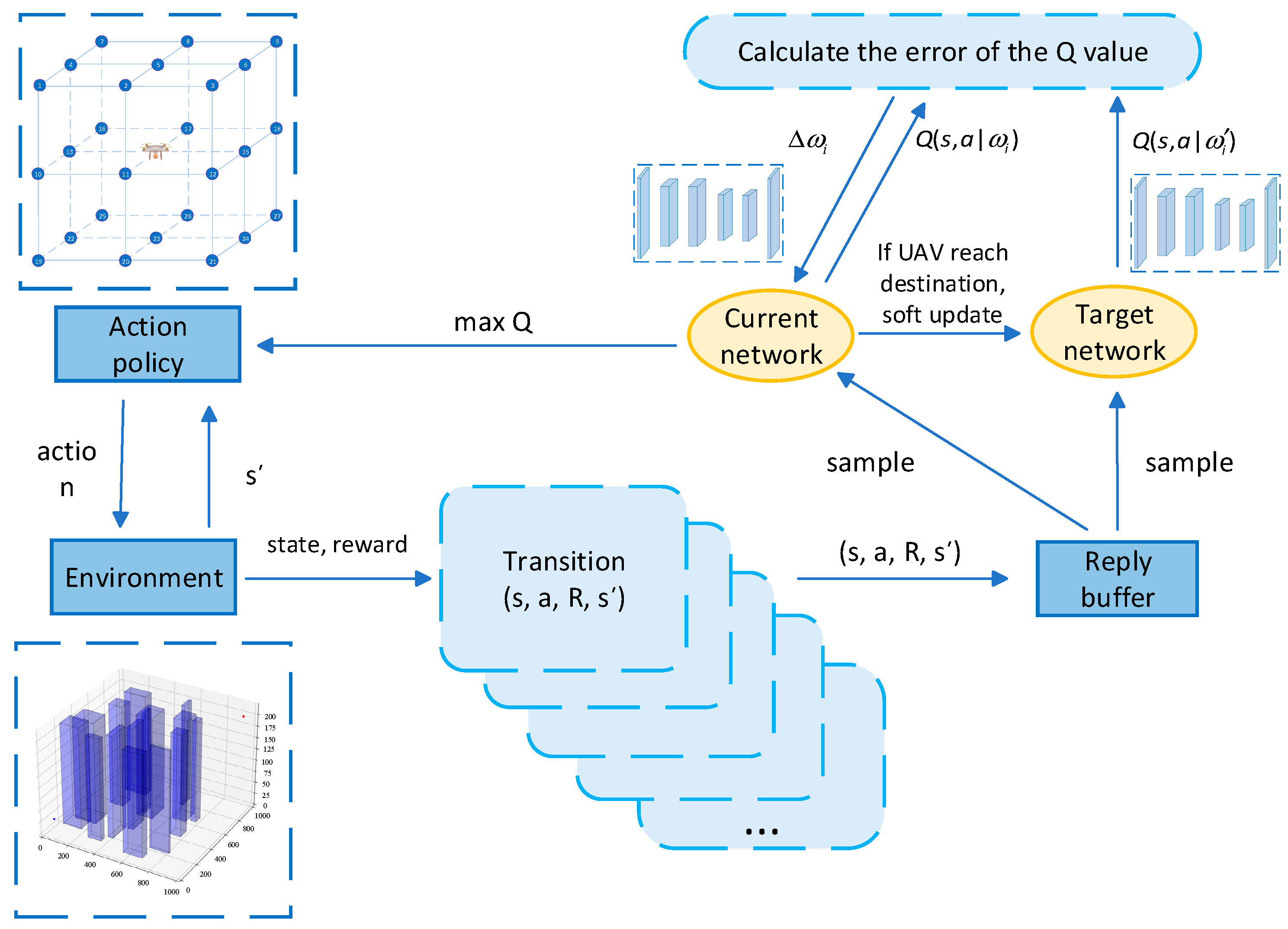
In this study, the Random Obstacle Training Linear Soft Update Meritocracy Double DQN (ROLSM-DDQN) algorithm described above is employed, and the current position of the UAV, the flight direction, the situation of the neighboring grids of obstacles, and the distance to the target point are used as the input states. The algorithm plans the path of the UAV. The algorithm’s framework and neural network architecture in this paper are shown in Figure 4 and Figure 5.

3.5. Reward Function

Within this algorithmic framework, the reward function plays a pivotal role in gauging the correctness of the UA’s actions. Positive rewards are assigned when the UAV executes actions to help it reach the target. In contrast, negative rewards are assigned if the UAV deviates from the target, encounters obstacles, or exceeds the specified steps. A composite reward function is introduced to address the challenges posed by dense urban environments and the resistance posed by wind during flight.

Each action executed by the UAV corresponds to a step. The steps are set to a negative reward to incentivize the UAV to get as close as possible to the target. In contrast, the difference in the distance between the start and target points and the length of the current position from the target point is set to a positive reward. The goal is to make the rewards higher when the UAV is close to the target, thus prompting it to take fewer steps out and earn higher rewards. The design of this composite reward function helps to optimize the flight path of the UAV so that it can perform better in complex urban environments. The $R_1$ is given by:

$$R_1=k_1(d_o-d_t)-k_2\mathrm{steps}$$

(17)

where $d_o$ denotes the distance from the start point to the target point, and $d_t$ denotes the distance from the current position to the target point. $k_1$ and $k_2$ are the parameters to balance the step reward and distance reward.

Considering the effect of ambient winds, it may be less labor-intensive to fly in the wind direction. The reward function also introduces the angle between the direction of the flight and the wind direction; the smaller the angle, i.e., the closer the direction of the flight is to the wind direction, the higher the reward. This can be quantified by the cosine and sine functions, which optimize flight movement for higher rewards when flying. The $R_2$ is given by:

$$R_2=k_3{F}_w(\cos {\theta }_1-\sin {\theta }_1)$$

(18)

where ${\theta }_1$ is the angle between the UAV flight direction and the wind direction, and $F_w$ is the wind magnitude, the same as in Equation (8), and $k_3$ is the weighting factor. Additionally, in the vertical direction, the rewards for ascending and descending differ due to the effects of the UA’s gravity. The ascending of the UAV requires it to overcome gravity and therefore a negative reward is needed. While the descendent of the UAV needs a positive reward due to the relative effort savings. The $R_3$ is given by:

$$R_3=-k_{4}dz$$

(19)

where $dz$ is the displacement of the UAV in the vertical direction after taking action $a$, the same as that of Equation (8), and $k_4$ is the weighting factor. In addition, when the UAV is stationary, a larger penalty is used to prevent the UAV from stalling for a long time. The $R_4$ is given by:

$$R_4=\left\{\begin{array}{ll}-100& \mathrm{if}\mathrm{standstill}\\ 0& \mathrm{if}\mathrm{not}\mathrm{standstill}\end{array}\right.$$

(20)

The UAV also receives a large penalty when it exceeds its maximum steps, thus directing it to explore a more reasonable path, and the episode will end. The $R_5$ is given by:

$$R_5=\left\{\begin{array}{ll}-200& \mathrm{Exceeding}\mathrm{the}\mathrm{maximum}\mathrm{steps}\\ 0& \mathrm{No}\mathrm{Exceeding}\end{array}\right.$$

(21)

A large penalty is assessed when the UAV collides and the current training episode is ends. The $R_6$ is given by:

$$R_6=\left\{\begin{array}{ll}-200& \mathrm{if}\mathrm{collision}\\ 0& \mathrm{if}\mathrm{not}\mathrm{collision}\end{array}\right.$$

(22)

A generous positive reward will be awarded when the UAV target point is reached, which will also mark the completion of the mission, and the episode will end. The $R_7$ is given by:

$$R_7=200$$

(23)

The composite reward function has three cases since the UAV has three terminal states. They are denoted as

$$R=\left\{\begin{array}{ll}-200& \mathrm{Exceeding}\mathrm{the}\mathrm{maximum}\mathrm{steps}\mathrm{or}\mathrm{collision}\\ R_1+R_2+R_3+R_4& \mathrm{No}\mathrm{Exceeding}\mathrm{or}\mathrm{not}\mathrm{collosion}\end{array}\right.$$

(24)

$$R=\left\{\begin{array}{ll}200& \mathrm{if}\mathrm{done}\\ R_1+R_2+R_3+R_4& \mathrm{if}\mathrm{not}\mathrm{done}\end{array}\right.$$

(25)

In summary, this composite reward function considers multiple factors, including distance, wind direction, vertical motion, steps, and collision, to provide explicit incentives and constraints for the UA’s behavior in a DRL algorithm for more optimal flight path planning. Algorithm 1 gives a pseudo-code for ROLSM-DDQN in wind-disturbed and urban-dense environments.

Algorithm 1: ROLSM-DDQN for UAV path planning

Input: the number of episodes $T$, UAV action space set $A$, the discount factor $\gamma$, learning rate $\alpha$, the exploration probability $\epsilon$, evaluation network parameters $\omega$, target network parameters ${\omega }^{\prime }$, buffer capacity $D$, batch size $N$, the replay of experience size $M$, soft update rate $\tau$, steps $n$; Initialization: empty buffer capacity $D$, evaluation network parameters $\omega$, target network parameters ${\omega }^{\prime }$, the replay of experience size $M=0$;

Output: network parameters $\omega$; For $i=1:T$ do

$n=0$, reset the environment;

While $True$ do

$n=n+1,M=M+1$

Select action $a_t\in A$ according to $\epsilon -\mathrm{greedy}$ policy;

Execute $a_t$ and transfer to next stats $s_{n+1}$;

Obtain reward $R_n$;

$D\leftarrow \left\{s_n,a_n,R_n,s_{n+1}\right\}$

If UAVs reach terminal states, then Break

End if

If $M\ge N$ and $n\%5=0$, then

Sample $N$ data from buffer capacity $D$

For $j=1:N$ do

$y_j=R_n+\gamma Q^{\prime }(s_{n+1},\arg {\max }_{a^{\prime }}Q(s_{n+1},a_n,\omega ),{\omega }^{\prime })$

End for

$L(\omega )=\frac{1}{N}{\displaystyle \sum _{j=1}^N(y_j}-Q(s_n,a_n,\omega ){)}^2$

${\omega }^{\prime }=\omega -\alpha \frac{dL}{d\omega }$

End if

If  $i\le \frac{T}{2}$, then

${\omega }^{\prime }=\tau \omega +(1-\tau ){\omega }^{\prime }$

Else

If UAV did not reach destination, then

Maintain the last episode’s ${\omega }^{\prime }$

Else

${\omega }^{\prime }=\tau \omega +(1-\tau ){\omega }^{\prime }$

End if

End if End while

$i=i+1$

End for

4. Simulation and Comparison Studies

In this section, several dense urban 3D environments are established, and various obstacle avoidance experiments are conducted. To be closer to the real urban environment, a 3D space of 1000 m × 1000 m × 220 m is established in this paper. As shown in Figure 6, the blue and red points represent the start and the target points, respectively, and the blue translucent rectangles represent the buildings. The buildings are distributed in a moderately dense manner, corresponding to practical application scenarios. The wind direction of the whole environment is on the positive x-axis, and the wind is fixed. The algorithm proposed in Section 3 is utilized in this paper to train the agent, which receives information about the agent’s current position, the neighboring grid obstacle situation, and the wind direction. To enhance the agent’s exploratory ability, especially in the early stages, an ε-greedy strategy is used, denoted as:

$$\pi (a|s)=\left\{\begin{array}{ll}uniform,& \mathrm{with}\mathrm{probability}\epsilon ;\\ \underset{a\in A}{\arg \max }Q(s,a|\theta ),& \mathrm{with}\mathrm{probability}1-\epsilon ;\end{array}\right.$$

(26)

where $\epsilon$ is a probability value. The probability that strategy $\pi$ selects an action value to maximize is $1-\epsilon$, while the probability that strategy $\pi$ selects another action is $\epsilon$, and the probability of selecting all other actions is equal. As training progresses, $\epsilon$ needs to be gradually reduced to decrease the agent’s exploration capability and balance the agent’s exploitation and exploration. The simulation parameters are summarized in

Table 1. Training parameters of the simulation.

Parameters	Value
The episodes of training	20,000
$\mathrm{Learning}\mathrm{rate}\alpha$	0.0005
$\mathrm{Minimal}\mathrm{Greedy}\epsilon$	0.01
$\mathrm{buffer}\mathrm{capacity}D$	100,000
$\mathrm{Batch}\mathrm{size}N$	1280
Maximum number of steps per episode	1450
$\mathrm{the}\mathrm{discount}\mathrm{factor}\gamma$	0.2

. The probability $\epsilon$ is minimized when episodes reach 5000, following which $\epsilon$ remains fixed at 0.01 in subsequent episodes.

4.1. Comparative Simulation of Different Random Obstacle Densities Training

To investigate the effect of different random obstacle densities on the algorithm’s training performance, four different random obstacle densities are compared and analyzed in this experiment. The difficulty levels of the environment are set to be $level=5$, $level=12$, $level=20$, $level=28$ in this experiment, respectively. During the training process, the number of obstacles is determined by these levels.

Each algorithm with a different level has been trained to conduct path planning for the illustrated scenarios in Figure 6, and the results are shown in

Table 2. Comparison results of different random obstacle densities training.

Comparisons	Score	Steps	Cost (Wh)	Path Length (m)
$\mathrm{ROLS}-\mathrm{DDQN}\mathrm{with}level=5$	3012.5115	1120	1132	152.9292
$\mathrm{ROLS}-\mathrm{DDQN}\mathrm{with}level=12$	3125.6443	1050	1046	141.6620
ROLS-DDQN with $level=20$	2921.0920	1160	1180	156.3899
$\mathrm{ROLS}-\mathrm{DDQN}\mathrm{with}level=28$	2844.0848	1210	1228	161.6268

. Since the scenario is relatively simple when the ROLS-DDQN with $level=5$ is trained, the path planning falls into a locally optimal solution when a slightly complex environment is encountered. In contrast, the ROLS-DDQN with $level=20$ fails to reach the target due to the overly complex obstacle environment, resulting in training failure. It negatively affects the neural network, lacks stability, and performs even worse than the ROLS-DDQN with $level=5$. The same goes for ROLS-DDQN with $level=28$. However, the ROLS-DDQN with $level=12$ has moderate environmental obstacles, which can match the difficulty of the environment shown in Figure 6. Therefore, this algorithm performs best in this experiment.

Compared to the ROLS-DDQN with $level=5$, the steps, the cost, and the path length of the ROLS-DDQN with $level=12$ are reduced respectively by 6.67%, 8.22%, and 7.95%. Meanwhile, compared to the ROLS-DDQN with $level=20$, they are still reduced by 9.48%, 12.81%, and 10.40%, respectively. Compared to the ROLS-DDQN with $level=28$, they are reduced by 9.48%, 12.81%, and 10.40%, respectively. Therefore, $level=12$ is suitable for this obstacle density and will be used for the subsequent simulation experiment training.

4.2. Comparative Simulation of Different Types of Soft Update Methods

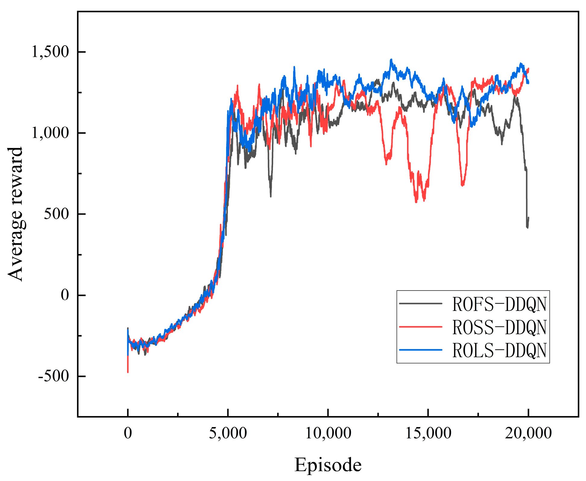
To examine the utility of the linear transformation soft update parameter in DRL, comparative experiments with three algorithms, Random Obstacle Fixed Soft Update DDQN (ROFS-DDQN), Random Obstacle Segmented Soft Update DDQN (ROSS-DDQN), and Random Obstacle Linear Soft Update DDQN (ROLS-DDQN), are conducted in this section. Their specific values are detailed in

Table 3. Different types of soft update rates and values.

Name	Value
$\mathrm{Linear}\mathrm{soft}\mathrm{update}\mathrm{rate}\tau$	$\tau$ $=0.008-i\_episode$ $*3*10*(-7)(i\_episode$ is the number of DRL training sessions)
$\mathrm{Segmented}\mathrm{soft}\mathrm{update}\mathrm{rate}\tau$	$\tau$ $=0.008(i\_episode$$<\mathrm{10,000});\tau$ $=0.002(i\_episode$ ≥ 10,000)
$\mathrm{Fixed}\mathrm{soft}\mathrm{update}\mathrm{rate}\tau$	$\tau$ = 0.005

. The average reward variations in iterations are shown in Figure 7.

Among these algorithms, the average reward of the ROLS-DDQN converges the smoothest. In comparison, the average reward of the ROFS-DDQN undergoes a sharp drop around 18,000 episodes and fails to converge before 20,000 episodes. The average reward of the ROSS-DDQN achieves ultimate convergence but encounters severe fluctuations between 12,500 and 17,500 episodes.

In this simulation, the soft update rate $\tau$ is critical. Since setting the value of the soft update rate to 0.005 achieves a desirable effect in this experiment, the simulation experiment is carried out with τ = 0.005. The adjustment of the latter half of the ROSS-DDQN’s $\tau$ is out of sync with the training dynamics, leading to instability and inefficiency. The ROFS-DDQN’s fixed $\tau$ worsens the performance and leads to unreasonable convergence. Conversely, the ROLS-DDQN dynamically adapts $\tau$ throughout the training process and continuously reduces it. This adaptive improvement maintains the algorithm’s stability and leads to reasonable convergence results.

Examining the overall performance, ROLS-DDQN is the best performer, followed by ROSS-DDQN, while ROFS-DDQN performs the worst. The outcome validates the significance of the linear transformations on the soft update rate.

4.3. Comparative Simulation of the Meritocracy Mechanism

To demonstrate the impact of the meritocracy mechanism and the advantages of DDQN, Random Obstacle Linear Soft Update Meritocracy DDQN (ROLSM-DDQN), ROLS-DQN, and ROLS-DDQN are compared in this section.

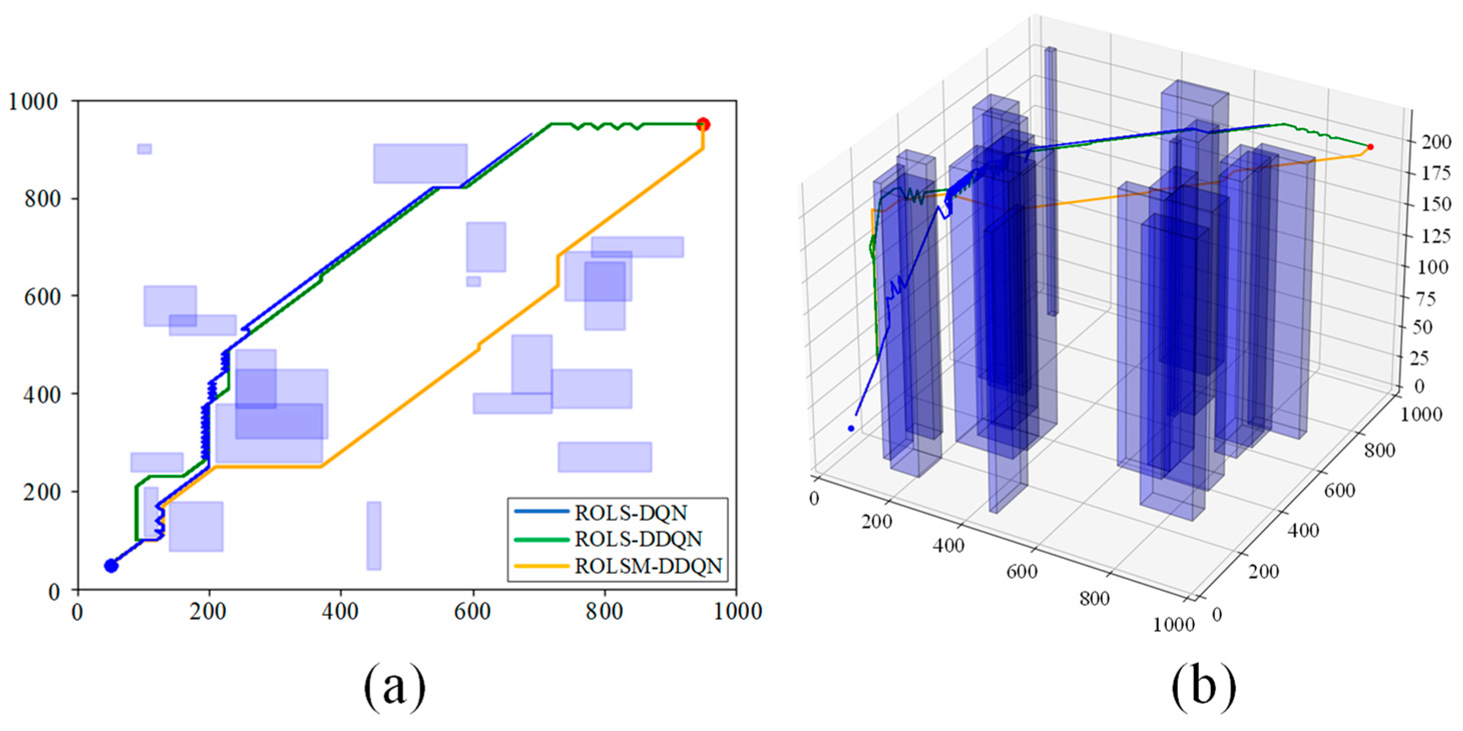
The visual representations in Figure 8 depict the aerial and 3D trajectories of the respective algorithms, respectively. The trajectories of the ROLS-DQN show excessive turns and exceed the step limit, causing the metrics of the ROLS-DQN to be meaningless. Conversely, the ROLS-DDQN and ROLSM-DDQN show more reasonable trajectories. The overestimation problem of the ROLS-DQN affects its training effectiveness, whereas the ROLS-DDQN and ROLSM-DDQN mitigate this issue by improving decision-making, convergence, and replay utilization. These benefits improve the stability and efficiency of training, yielding desirable results. The ROLS-DDQN encounters multiple obstacles and reaches the target, but its performance can be improved. The ROLSM-DDQN outperforms the ROLS-DDQN by selecting a direct path with fewer obstacles. In this context, the meritocracy mechanism plays an essential role. It removes training failures while maintaining the integrity of previous neural network parameters. Consequently, during unsuccessful UAV training, the neural network parameters are not affected by change, and during successful training, the mechanism continually optimizes the trajectory.

The comprehensive path planning details are presented in

Table 4. Comparison results of the meritocracy mechanism.

Comparisons	Score	Steps	Cost (Wh)	Path Length (m)
ROLS-DQN	—	—	—	—
ROLS-DDQN	2921.0920	1160	1180	156.3899
ROLSM-DDQN	3125.6443	1050	1046	141.6620

. The ROLSM-DDQN establishes significant advantages in steps, cost, and path length metrics. Compared with the ROLS-DDQN, they are reduced by 9.77%, 12.58%, and 13.68% in the ROLSM-DDQN. These results validate the effectiveness of the meritocracy mechanisms in optimizing path planning, reducing unnecessary actions, and improving overall effectiveness.

4.4. Comparative Simulation of the ROLSM-DDQN and the Traditional Algorithms

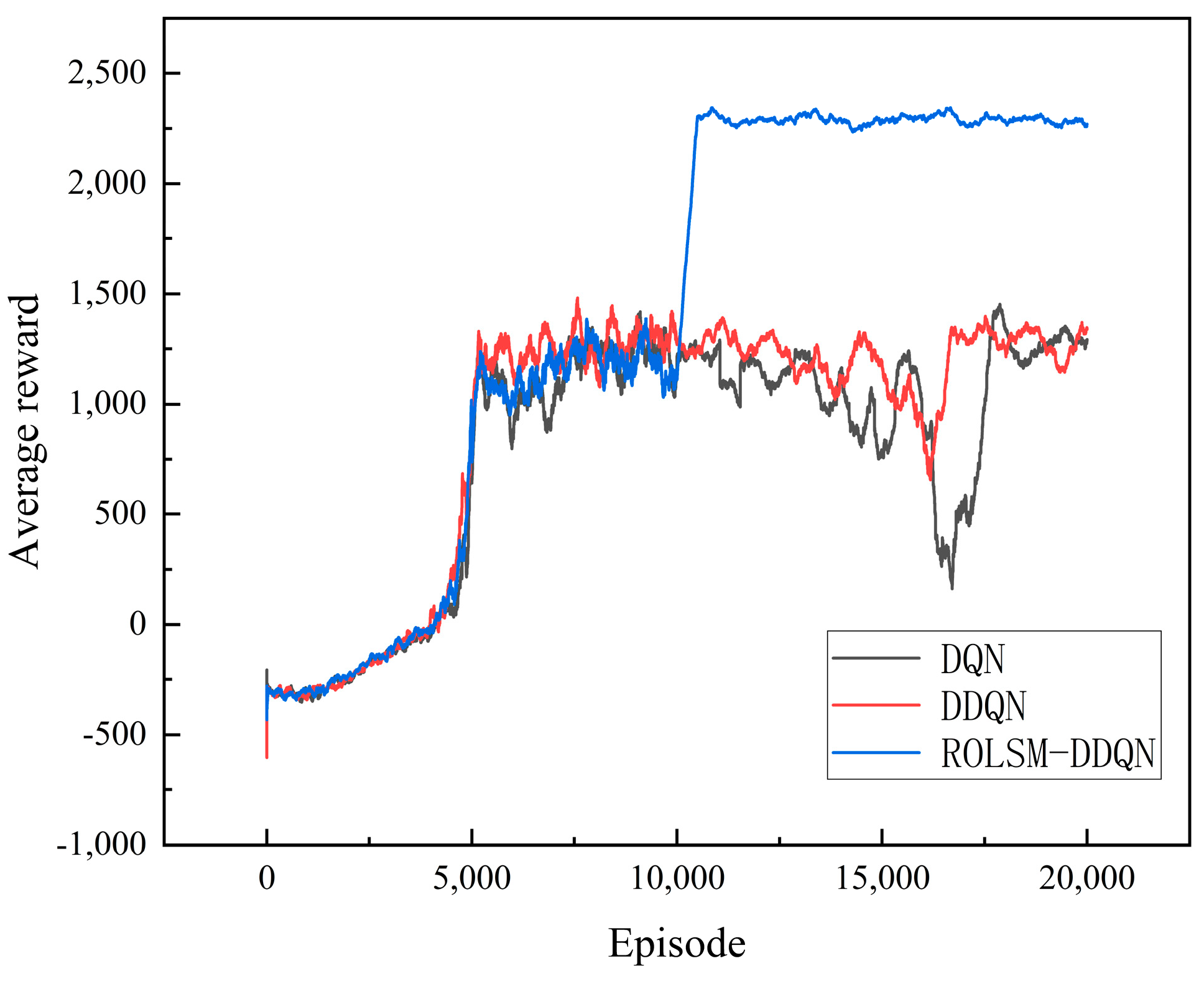
To validate the significance of the introduced random obstacle training, linear soft update rate, and meritocracy mechanism for DRL, a comparative analysis of the traditional DQN, the traditional DDQN, and the ROLSM-DDQN is conducted in this section. The average reward variations of these algorithms are shown in Figure 9. Although the entire training is conducted in a specific environment, the average rewards of the DQN and DDQN fluctuate widely between 15,000 and 17,500 episodes, and the average rewards of the DQN reach a minimum average reward value close to zero, which seriously affects stability and performance. This simulation demonstrates the inherent instability of DQN, and DDQN. Therefore, they are unsuitable for the experimental scenarios described in this paper.

In contrast, the average reward of the ROLSM-DDQN goes stably after 10,000 episodes and outperforms the others in the later stages. The random obstacle training, linear soft update, and meritocracy mechanism play critical roles. The random obstacle training enables the algorithm to generalize to different scenarios with varying obstacles. The meritocracy mechanism is introduced after 10,000 episodes. It cleverly discards unsuccessful training results and utilizes the average reward gained from successful training instances while preserving the previous neural network parameters. In the latter half of its iteration, linear soft update works only after successful training, further refining the network architecture.

In summary, this experiment further affirms the significance of the random obstacle training, linear soft update, and meritocracy mechanisms in DRL. These strategies not only enhance the stability of the algorithm but also improve its performance by effectively dealing with faulty situations during the training process.

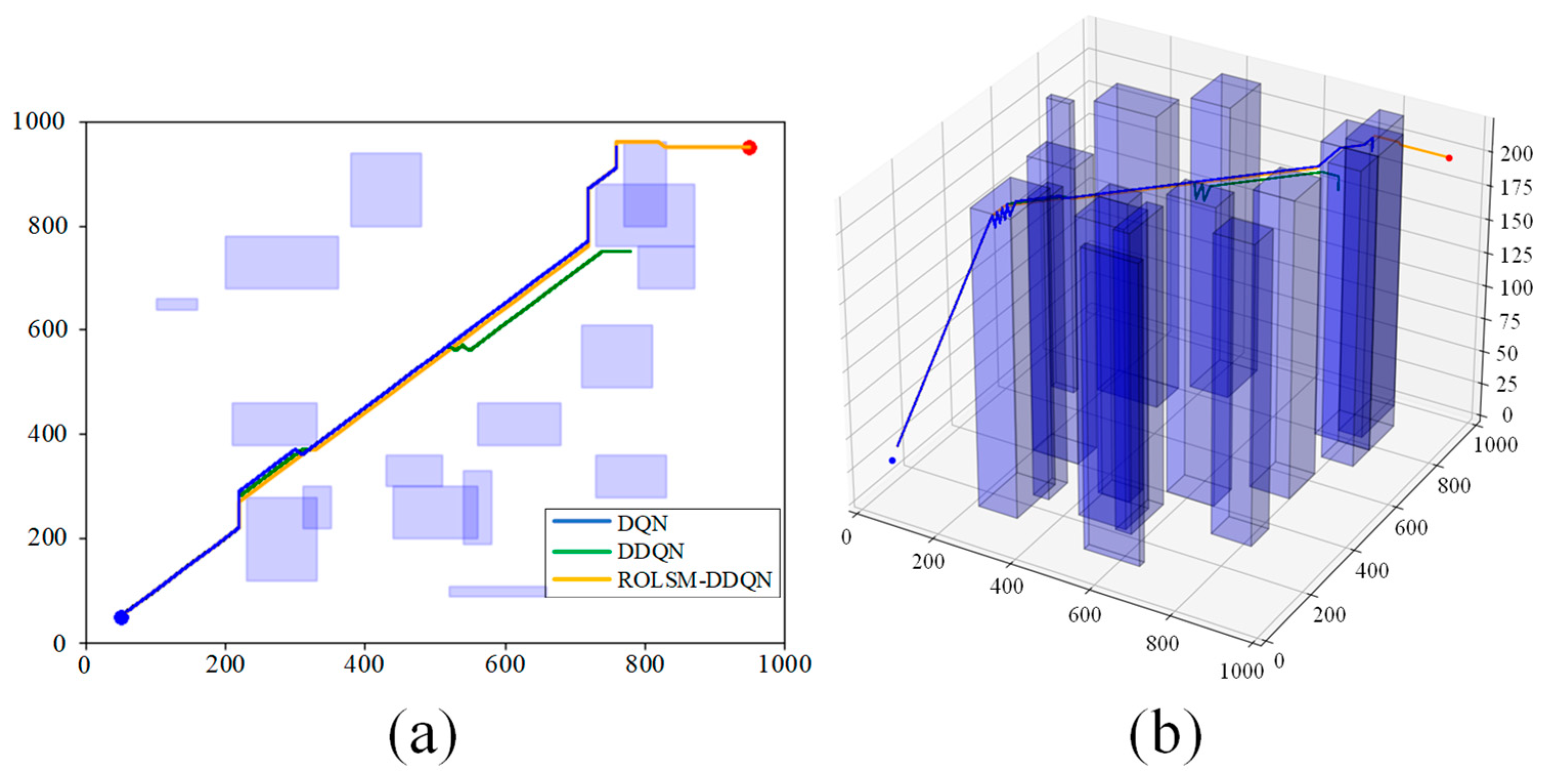
In this experiment phase, two map scenarios with different obstacles distribution suitable for real dense cities are established, and comprehensive comparisons of the ROLSM-DDQN, DQN, and DDQN are performed to evaluate their performance on reward, steps, cost, and path length. The results are detailed in Figure 10 and Figure 11, and

Table 5. Comparison Results of Path Planning.

Map No.	Model Name	Reward	Steps	Cost (Wh)	Path Length (m)
1 (Figure 10)	DQN	2993.2383	1120	1136.0	1578.14
	DDQN	2987.6965	1110	1125.31	1577.66
	ROLSM-DDQN	3125.5443	1050	1046.0	1416.62
2 (Figure 11)	DQN	—	—	—	—
	DDQN	—	—	—	—
	ROLSM-DDQN	3079.9054	1110	1110.0	1458.12

.

Map No. 1 is a training environment for two traditional algorithms, the same as Figure 6. However, the DDQN approach leads to multiple turns and off-target points, increasing steps, path length, and energy consumption, making it a suboptimal strategy. While the trajectory of the DQN overlaps with that of the ROLSM-DDQN, the DQN also suffers from excessive turns during the path planning process, leading to a degradation in performance. In contrast, the ROLSM-DDQN follows mainly a direct trajectory towards the destination, which makes it satisfactory on the map. Compared to the DQN, the steps, the cost, and the path length of the ROLSM-DDQN are reduced by 6.25%, 8.60%, and 10.23%, respectively. Similarly, they achieve 5.41%, 7.58%, and 10.23% reductions, respectively, compared to the DDQN. These results highlight the effectiveness of the ROLSM-DDQN in complex obstacle scenarios.

In Map No. 2, obstacles are randomly changed for testing the above algorithms after training. The difficulty level of the changed obstacles is equivalent to Map No. 1. However, only the ROLSM-DDQN succeeds in reaching the goal with lower steps and path length, thus earning a higher reward. The DDQN enters the dead center of the obstacle and fails in path planning. The DQN’s path matches that of the ROLSM-DDQN but suddenly loses direction before the last obstacle and fails to reach the target, exceeding the step limit. The experiment illustrates that the algorithm in the same obstacle training environment cannot generalize to different scenarios, and introducing random obstacle training enables the algorithm to achieve the desired results.

In conclusion, the comprehensive simulation results in this paper confirm the significantly satisfactory performance of the introduced ROLSM-DDQN method in multiple scenarios. It can be a robust and effective technique for solving UAV path-planning problems in dense urban environments.

5. Conclusions

In this paper, the ROLSM-DDQN algorithm is proposed to solve the UAV path planning problem in dense urban scenarios. Initially, introducing the random obstacle training method allows the algorithm to generalize to different scenarios with different obstacles, improving the algorithm’s robustness and adaptability. Then, the proposed linear soft update strategy smoothly updates the neural network parameters, which helps improve training stability and convergence. The composite reward function considers multiple factors, including distance, wind direction, wind resistance, collision, and vertical motion, closely related to the energy consumption model. It achieves a more optimal flight path planning strategy. Additionally, the meritocracy mechanism proposed in this paper helps maintain parameter stability, improving training efficiency and stability. The ROLSM-DDQN demonstrates a significant superiority in metrics as a result of the steps, energy consumption, and path length. Compared to the traditional DQN, the steps, the cost, and the path length of the ROLSM-DDQN are reduced by 5.41%, 7.58%, and 10.23%, respectively. Compared to the traditional DDQN, they achieve 6.25%, 8.60%, and 10.23% reductions, respectively. Simulation experiment results verify the algorithm’s effectiveness for path planning in dense urban scenarios, successfully solving the path planning problem in large-scale and complex environments.

However, the ROLSM-DDQN algorithm belongs to offline planning, which requires anticipation of global information, cannot adapt to real-time demands, and does not apply to dynamic environments. To address the above limitations, how to make DRL more suitable for dynamic environments and real-time scenarios will be further explored in future research. First, research will be conducted on how to build models that can handle time-varying environments to better adapt to real-time requirements. By capturing the dynamic changes in the state of the environment, more flexible algorithms will be designed so that strategies can be adjusted promptly to adapt to changes in the environment. Secondly, new obstacle avoidance strategies and methods will be explored to cope with the appearance and movement of dynamic obstacles. It involves the development of real-time path planning, obstacle detection, and avoidance techniques to ensure safe navigation in complex environments. In addition, efforts will be made to optimize the computational efficiency and real-time performance of the algorithms so that they can respond and make decisions quickly in real-world applications. Through these improvements and extensions, it is expected that more practical and adaptable DRL algorithms can be developed so that they can play a greater role in practical applications.