Article

Well Logging Reconstruction Based on a Temporal Convolutional Network and Bidirectional Gated Recurrent Unit Network with Attention Mechanism Optimized by Improved Sand Cat Swarm Optimization

1
Hebei Instrument & Meter Engineering Technology Research Center, Hebei Petroleum University of Technology, Chengde 067000, China
2
Department of Computer and Information Engineering, Hebei Petroleum University of Technology, Chengde 067000, China
3
State Key Laboratory of Nuclear Resources and Environment, East China University of Technology, Nanchang 330013, China
*
Author to whom correspondence should be addressed.
Energies 2024, 17(11), 2710; https://doi.org/10.3390/en17112710
Submission received: 30 March 2024 / Revised: 19 May 2024 / Accepted: 28 May 2024 / Published: 3 June 2024
(This article belongs to the Section H: Geo-Energy)

Abstract

:
Geophysical logging plays a very important role in reservoir evaluation. In the actual production process, some logging data are often missing due to well wall collapse and instrument failure. Therefore, this paper proposes a logging reconstruction method based on improved sand cat swarm optimization (ISCSO) and a temporal convolutional network (TCN) and bidirectional gated recurrent unit network with attention mechanism (BiGRU-AM). The ISCSO-TCN-BiGRU-AM can process both past and future states efficiently, thereby extracting valuable deterioration information from logging data. Firstly, the sand cat swarm optimization (SCSO) improved by the variable spiral strategy and sparrow warning mechanism is introduced. Secondly, the ISCSO’s performance is evaluated using the CEC–2022 functions and the Wilcoxon test, and the findings demonstrate that the ISCSO outperforms the rival algorithms. Finally, the logging reconstruction method based on the ISCSO-TCN-BiGRU-AM is obtained. The results are compared with the competing models, including the back propagation neural network (BPNN), GRU, and BiGRU-AM. The results show that the ISCSO-TCN-BiGRU-AM has the best performance, which verifies its high accuracy and feasibility for the missing logging reconstruction.

1. Introduction

Logging is a technique for determining the characteristics of underground rocks and fluids by means of sensors in boreholes [1,2,3,4]. When the logging instrument fails or the well wall is destroyed, the logging data in some sections will be missing. Repeated logging is often costly and difficult to achieve in a well that has already been completed. Therefore, the hunt for a precise technique to reconstruct logging data has enormous scientific significance. Many logging prediction methods have been proposed, such as empirical formulas [5] and multiple regression analysis [6]. These methods have achieved a certain effect of logging reconstruction under certain conditions, but they ignore the complex formation conditions. Therefore, it is difficult to meet the accuracy requirements of logging interpretation and reservoir characterization.
Machine learning methods have widely been used in geological parameter estimation and reservoir identification [7,8,9], and they have achieved better results than traditional statistical methods. Deep learning methods can extract complex features and can be used to solve complex nonlinear geological problems. Many scholars have applied deep learning methods to the research of logging curve reconstruction. For example, a generalized regression neural network is used in logging reconstruction experiments, which shows that the neural network method has a higher curve reconstruction accuracy than linear regression [10]. A deep confidence network provides a distinct benefit when it comes to the initialization of the network weight matrix and produces precise formation porosity prediction [11]. But the above approaches ignore the logging data’s association with depth.
The logging data set has the characteristics of sequential representation. Therefore, the time series model can be introduced to the prediction of missing logging data. A long short-term memory network (LSTM) is used for missing logging prediction, and it fully considers the depth-dependent fluctuation trend of the logging data [12]. However, an LSTM has shortcomings including a slow convergence speed and long training time. A gated recurrent unit network (GRU) has a more concise structure and can effectively solve the gradient disappearance problem [13]. Logging data involve a series of data with depth direction, and their variation trend has rich geological meaning. Due to the small sampling interval, logging data have a long-term correlation in time and space, but a traditional GRU can only predict the target data from one direction. A bidirectional gated recurrent unit network (BiGRU) can fully utilize pertinent data to rebuild the logging data by extracting the feature data from the front and back, respectively [14]. The attention mechanism is introduced to further enhance the influence of key information. A temporal convolutional network (TCN) has recursive and convolutional architecture and can be applied as a starting point for the model to process sequential data [15]. The SCSO is a new metaheuristic algorithm which has demonstrated outstanding performance [16]. However, it also has drawbacks, including unbalanced global exploration and a slow convergence speed. To enhance the SCSO, the variable spiral approach and sparrow warning mechanism are implemented. ISCSO can be applied to optimize hyperparameters of models to enhance the optimization performance.
In this paper, a combined model named TCN-BiGRU-AM is proposed to be applied in logging reconstruction. It primarily takes advantage of TCN, BiGRU, and AM’s benefits in processing time series data. A TCN can efficiently extract temporal information in features. A BiGRU is capable of obtaining the features’ contextual linkage. An AM is presented to better capture the long-range connections between features. An ISCSO can be used for the optimization of TCN-BiGRU-AM, which can further improve prediction performance. It can be found that the ISCSO-TCN-BiGRU-AM has excellent prediction performance for logging reconstruction than the competing models.
The main contributions are summarized as follows:
(1)
A TCN-BiGRU-AM initially takes advantage of a TCN’s superior parallel processing capabilities. Secondly, it takes advantage of a BiGRU’s capacity to extract the contextual correlation between characteristics. Furthermore, it makes use of an AM’s capability to extract internal self-correlation.
(2)
The variable spiral strategy and sparrow warning mechanism are first introduced to enhance the SCSO’s optimization capability. The ISCSO is used to optimize the hyperparameters of TCN-BiGRU-AM, thereby improving the prediction performance.
(3)
In engineering practice, ISCSO-TCN-BiGRU-AM significantly outperforms the competing models in missing logging reconstruction. The proposed model has effective practical implications and can successfully handle real industry needs.
The remaining part of this study is structured as follows: In Section 2, the principles of the TCN, BiGRU, AM, and ISCSO are presented. In Section 3, the superiority of the OCSSA is presented. In Section 4, the application of the ISCSO-TCN-BiGRU-AM is presented. Finally, Section 5 presents the conclusion of this paper.

2. Principles and Methods

2.1. TCN-BiGRU-AM

2.1.1. TCN

A temporal convolution network (TCN) is mainly composed of three components, including causal convolution, dilated convolution, and residual chunking [15]. Each structure has a detailed explanation, and they are each provided below.
(1)
Causal convolution
According to the features of time series, causal convolution suggests that the output depends on the historical input. When the input is X = x 1 , x 2 , ,   x T ,   X R n and the filter is F = f 1 ,   f 2 , ,   f k , the output Y T is expressed as Equation (1).
Y T = i = 0 k 1 F i · x T i
where k is the filter size, and T i is the direction of the past.
The size of the receptive field places restrictions on the causal convolution, which makes it effective only for short-history information prediction.
(2)
Dilated convolution
Dilated convolution is a convolution operation using the dilation factor d to solve the limited field of perception issue. When the input is X = x 1 , x 2 , ,   x T and the filter is F = f 1 ,   f 2 , ,   f k , the output Y T is expressed as Equation (2).
Y T = i = 0 k 1 F i · x T d · i
where k is the filter size, and T d · i is the direction of the past.
When the convolution kernel size is 3 and the dilation factors are 1, 2, and 4, respectively, the framework of the dilated causal convolution is as shown in Figure 1.
The dilation factor is applied for interval sampling in dilated convolution. When d = 1 , it means that all of the input gets sampled. when d = 2 , the input is sampled every two points. The receptive field and expansion factor both grow as the number of layers increases. Dilated convolution can provide a broader receptive field with shallow networks.
(3)
Residual module
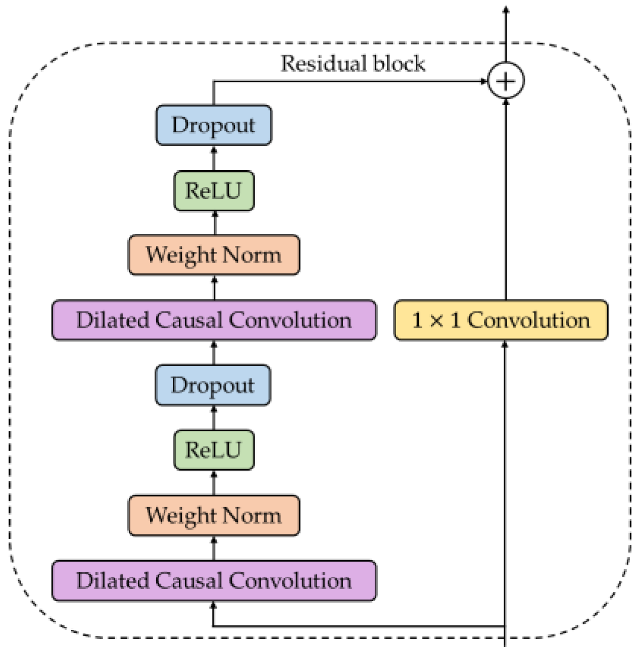
The residual module is displayed in Figure 2.
The purpose of the residual connection is to short-circuit the connection and add the features that were taken from the model to prevent the loss of significant original features during the information extraction process. Residual connections can help the model remain more stable when processing lengthy sequences, prevent gradients from disappearing, and preserve significant original characteristics that are lost during the extraction of deep features.

2.1.2. BiGRU-AM

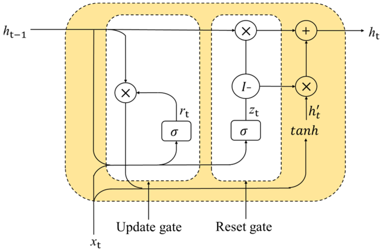
The framework of the GRU is shown in Figure 3.
At time t , the calculation process is expressed as follows:
r t = σ W r x x t + W r h h t 1 + b r
z t = σ W x z x t + W h z h t 1 + b z
h t = t a n h W x h x t + W h r t · h t 1 + b h
h t = z t · h t 1 + 1 z t · h t
where x t is the input at time t ; r t is the reset gate; z t is the update gate; h t is the hidden status; h t is the candidate hidden state; σ and t a n h are the activation functions; W x z , W h z , W x h , and W h are the related weight matrices; and b r , b z , and b h are the offset of the reset gate unit, the button to update the gate unit, and the candidate output, respectively.
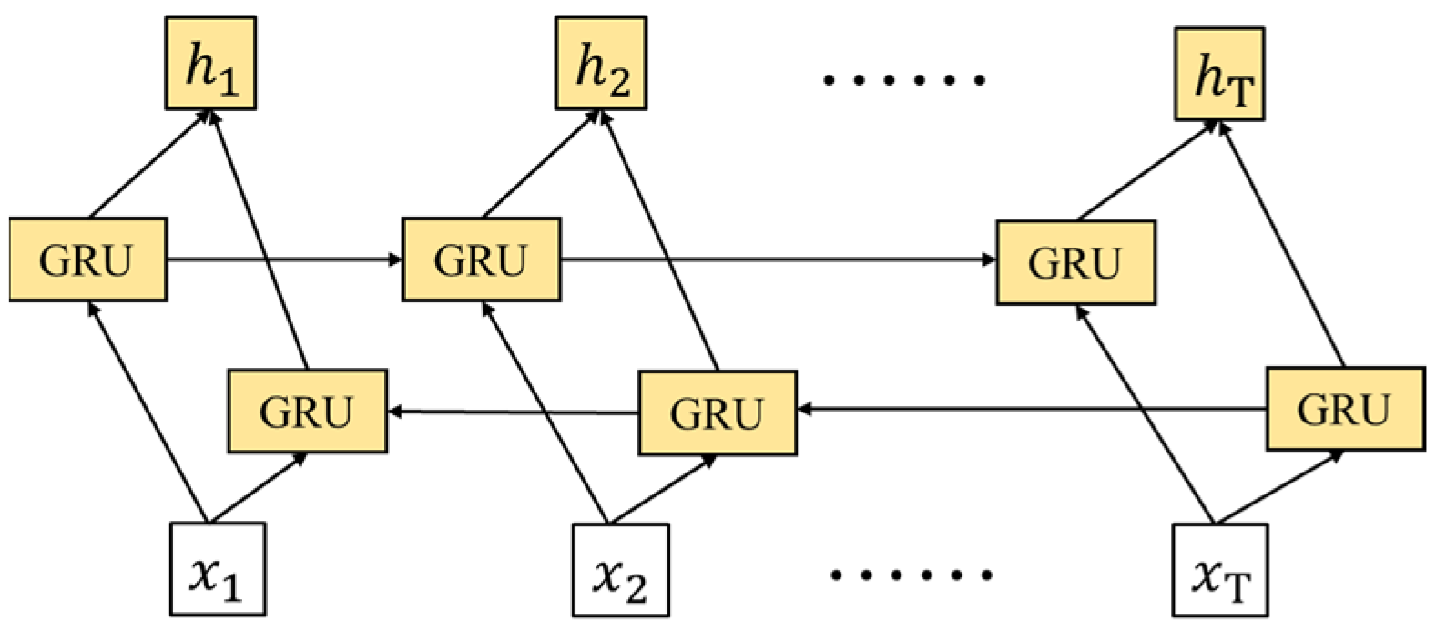
The BiGRU has hidden sequences forward ( h t = h 1 , h 2 , , h n ) and backward ( h t = h 1 , h 2 , , h n ). The final output is generated by combining the forward and backward hidden outputs, which are expressed as follows:
y t = σ w y h h t + w y h h t + b y
h t = σ w h x x t + w h h h t 1 + b h
h t = σ w h x x t + w h h h t + 1 + b h
where y t = h t , h t is the output of the bi-directional hidden layer.
The framework of the BiGRU is shown in Figure 4.
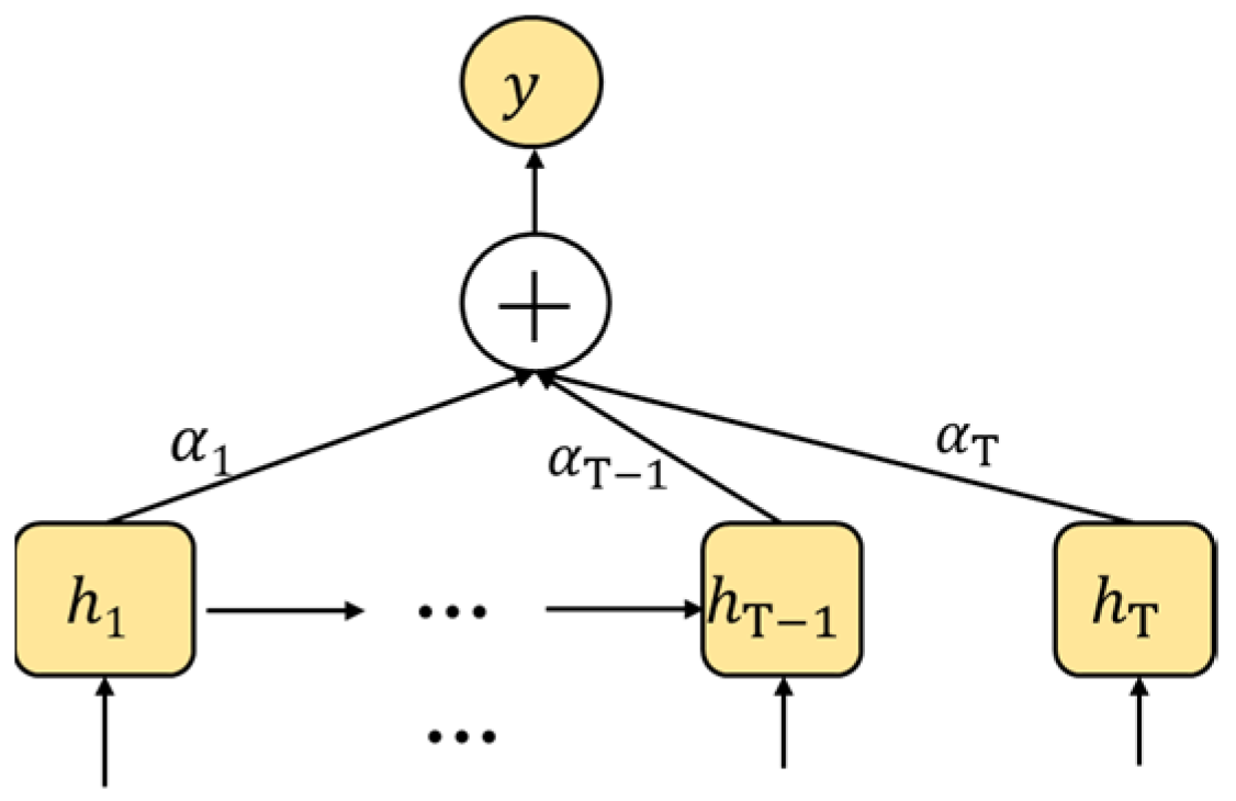
Attention mechanism (AM) is a data processing technique that can suppress irrelevant information and amplify relevant information. The framework of AM is shown in Figure 5.
The weight coefficient of AM is obtained as follows:
e t = u t a n h w h t
α t = e x p e t j = 1 t e j
s t = t = 1 i α t h t
where h t is the output of BiGRU, and α t is the attention probability distribution.

2.1.3. TCN-BiGRU-AM Flow Chart

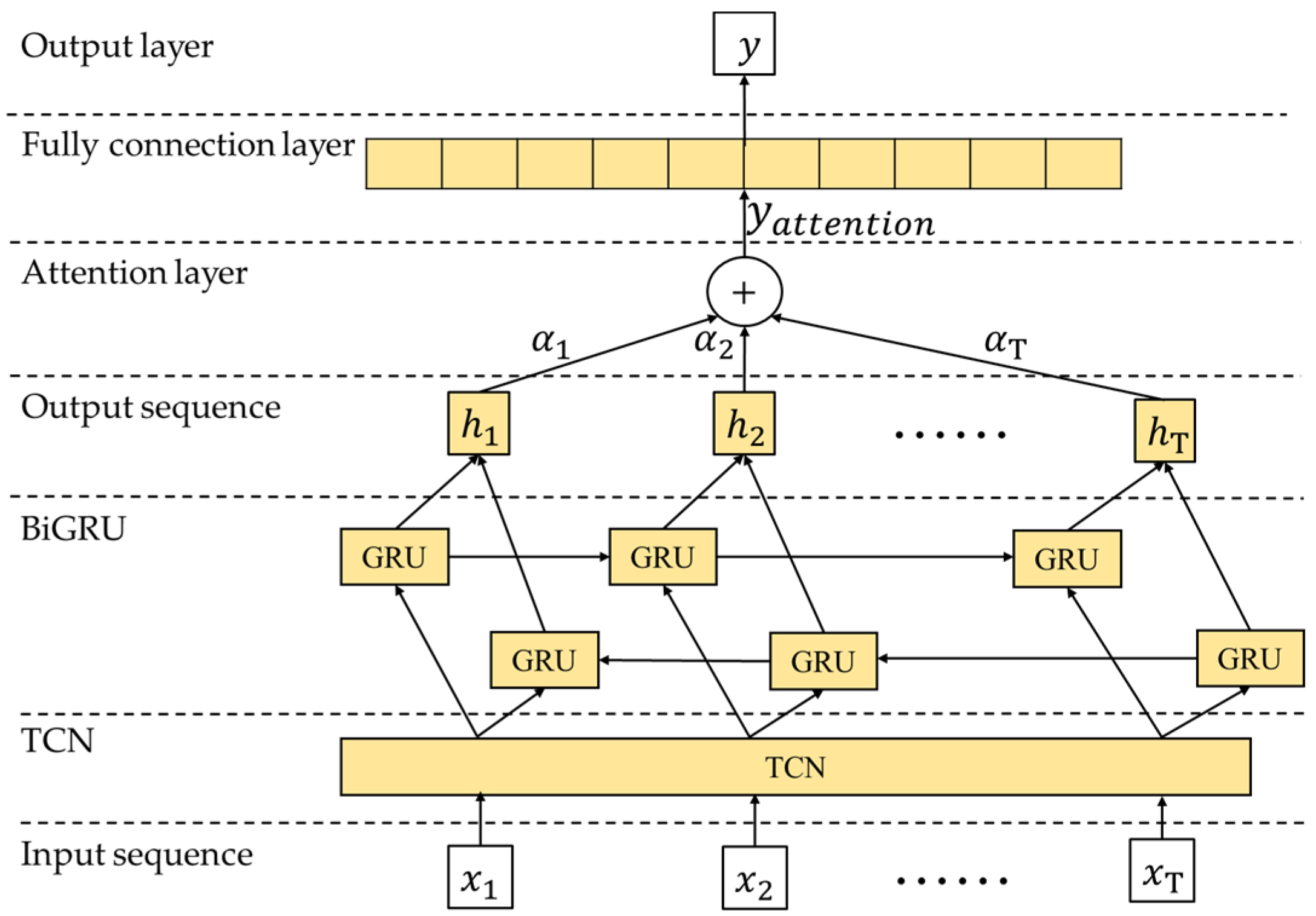
The framework of the TCN-BiGRU-AM is shown in Figure 6. The whole model structure is composed of six parts, including the input, TCN, BiGRU, AM, full connection, and output.

2.2. SCSO

Sand cat swarm optimization (SCSO) can be divided into exploration and exploitation phases [16].
When the sand cat swarm is initialized, the hunting activity begins. The conversion factor is represented as R , which can determine whether to enter the exploration or exploitation phase. The R can be calculated using Equation (13):
R = 2 r G · r a n d 0 , 1 r G
where r G is the sensitivity coefficient of sand cat swarm. The r G can be obtained from Equation (14):
r G = S M S M · t / T
where t is the current iteration. S M is the hearing coefficient, which simulates hearing characteristics. S M can be set to 2, or other values can be set according to the actual problem solving.
When R > 1, sand cat swarm started its exploratory phase. The position of the ith sand cat is updated according to Equation (15):
X i t + 1 = r i · X best t r a n d 0 , 1 · X i t
where X best t is the position of the optimal sand cat in the swarm at the tth iteration. r i is the sensitivity coefficient of the ith sand cat. The r i can be calculated using Equation (16):
r i = r G · r a n d 0 , 1
When R ≤ 1, the sand cat swarm started its exploitation phase. The position of the ith sand cat is updated according to Equation (17):
X i t + 1 = X best t r i · X rand t · c o s θ
where θ is a random angle in the range of 0° to 360°, simulating the sand cat’s exploitation behavior. X rand t is a random position, which is calculated using Equation (18):
X rand t = r a n d 0 , 1 · X best t X i t
Through the adaptive transformation of the exploration and exploitation, the effective balance of the two phases is achieved.

2.3. Improvement of SCSO

In the attack behavior of SCSO, the attack direction is determined by a random angle between 0 ° and 360 ° , but a large range of random angles has certain blindness, which will greatly reduce the optimization efficiency. In the search behavior of SCSO, the overall fitness as a measure of individual quality, and it cannot fully reflect the individual position in the space. In addition, for a coordinate that has converged to the optimal position in a certain dimension, the search behavior will cause it to oscillate around the optimal solution, resulting in the reduction in convergence efficiency. As a result, the next two methods are offered to enhance SCSO’s optimization performance.

2.3.1. Variable Spiral Strategy

In a variable spiral search [17], the spiral search strategy factor m is a parameter varying with the number of iterations, and the spiral shape is dynamically adjusted to broaden the global exploration area of the swarm.
The spiral search strategy factor m can be obtained from Equation (19):
m = e 5 c o s π 1 t t m a x
The variable spiral strategy is introduced to improve the position of the sand cat swarm in the exploration phase. It can be updated according to Equation (20):
X i t + 1 = e m l · c o s 2 π l · r i · X best t r a n d 0 , 1 · X i t
By integrating spiral exploration, the sand cat swarm can explore in the form of a spiral, expanding the ability to explore unknown areas, increasing the possibility of the algorithm jumping out of the local optimal, and effectively improving the global exploration performance.

2.3.2. Sparrow Warning Mechanism

The sparrow’s warning mechanism [18] can be applied to enhance the convergence speed of SCSO, which can be obtained using Equation (21):
X i t + 1 = X best t + b · X i t X best t                                       f i > f g X i t + k · X i t X worst t f i f w + ε                                             f i = f g
where X best t is the global optimal location. f i , f g , and f w are the current, best, and worst fitness values, respectively. When f i > f g , this suggests that the sand cat is nearing the periphery of its population and is susceptible to natural adversaries. When f i = f g , this means that the sand cat in the midst of the swarm is conscious of the threat and needs to stick near to others to avoid being caught. k represents the step control parameter and the direction in which the sparrow is moving.

2.3.3. ISCSO Flow

The flowchart of the ISCSO is shown in Figure 7.
The following are the precise steps:
Step 1: Initialize the population and set the relevant parameters.
Step 2: Update population’s optimal solution, the population’s worst solution, and individual optimal solution and calculation algorithm parameters, r G , r , and R .
Step 3: When R > 1 , the exploration phase is entered, the variable spiral strategy is introduced, and the search agent position is updated by Equation (20). When R 1 , the exploitation phase is entered, and the search agent position is updated by Equation (17).
Step 4: Add the sparrow warning mechanism and update the search agent position based on Equation (21).
Step 5: Repeat Step 2 to Step 4 until the conditions are met to stop training.

3. ISCSO Performance Test

3.1. Analysis of CEC–2022 Functions

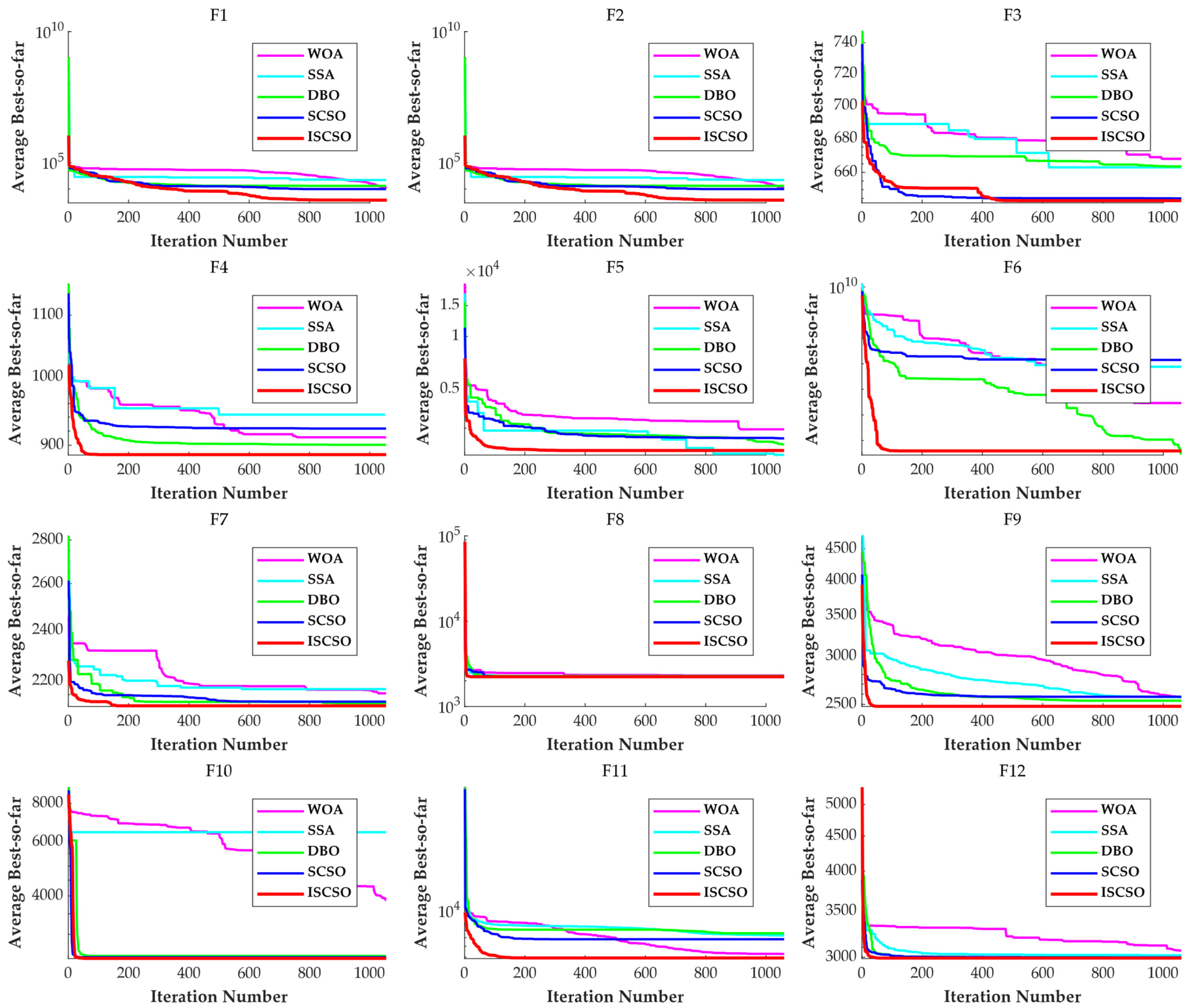
The performance evaluated by using the fitness value’s mean and standard deviation is displayed in Table 1. The ISCSO finds the better solution in F1–F4, F6–F9, and F10. For F5 and F11, ISCSO is not the best, but it is still in the lead. For F12, the ISCSO is similar to SCSO and the dung beetle optimizer (DBO) [17], but it is still superior to the sparrow search algorithm (SSA) [18] and whale optimization algorithm (WOA) [19]. It is evident from the experimental results that using the ISCSO is a better solution for solving the competition optimization issues than using the other algorithms.
The convergence curve is used to examine the ISCSO’s performance. The convergence curves for the ISCSO and the competing algorithms are displayed in Figure 8. It can be seen in Figure 8 that the ISCSO can obtain more satisfying mean fitness values at a faster rate of convergence.

3.2. Analysis of Rank Sum Test

The performance of the ISCSO is further discussed using the Wilcoxon test. Table 2 displays the p-values for the Wilcoxon tests between the ISCSO and the competing algorithms. The ISCSO differs greatly compared to the competing algorithms in the functions, including F1–F4 and F6–F10. For F5, the ISCSO is similar to WOA. For F11, the ISCSO is similar to SCSO, DBO, and WOA. For F12, the ISCSO is similar to SCSO and DBO. The improved performance of OCSSA is further explained by the analysis shown above.

4. Practical Application and Analysis

4.1. ISCSO-TCN-BiGRU-AM Prediction Flow

In the training of the TCN-BiGRU-AM, the parameter selection in traditional training is carried out manually based on experience, which is heavily influenced by individual preferences. The ISCSO can be utilized to obtain ideal parameters.
The following lists the specific steps of the ISCSO-TCN-BiGRU-AM.
Step 1: The data set is divided into two parts, training and testing, and the normalization is carried out by the max–min normalization method, which can be expressed as Equation (22):
x = x x m i n x m a x x m i n
where x is the actual value, x m a x and x m i n are the maximum and minimum values of x , respectively, and x is the normalized value.
Step 2: The root mean square error (RMSE) is selected as the objective function. RMSE is expressed as Equation (23):
R M S E = 1 N i = 1 N y k y ^ k 2
where y k and y ^ k are the true value and predicted value, respectively.
Step 3: The ISCSO is used to optimize the hyperparameters of TCN-BiGRU-AM.
Step 4: The TCN-BiGRU-AM is estimated with the optimal parameters.

4.2. Data Preparation

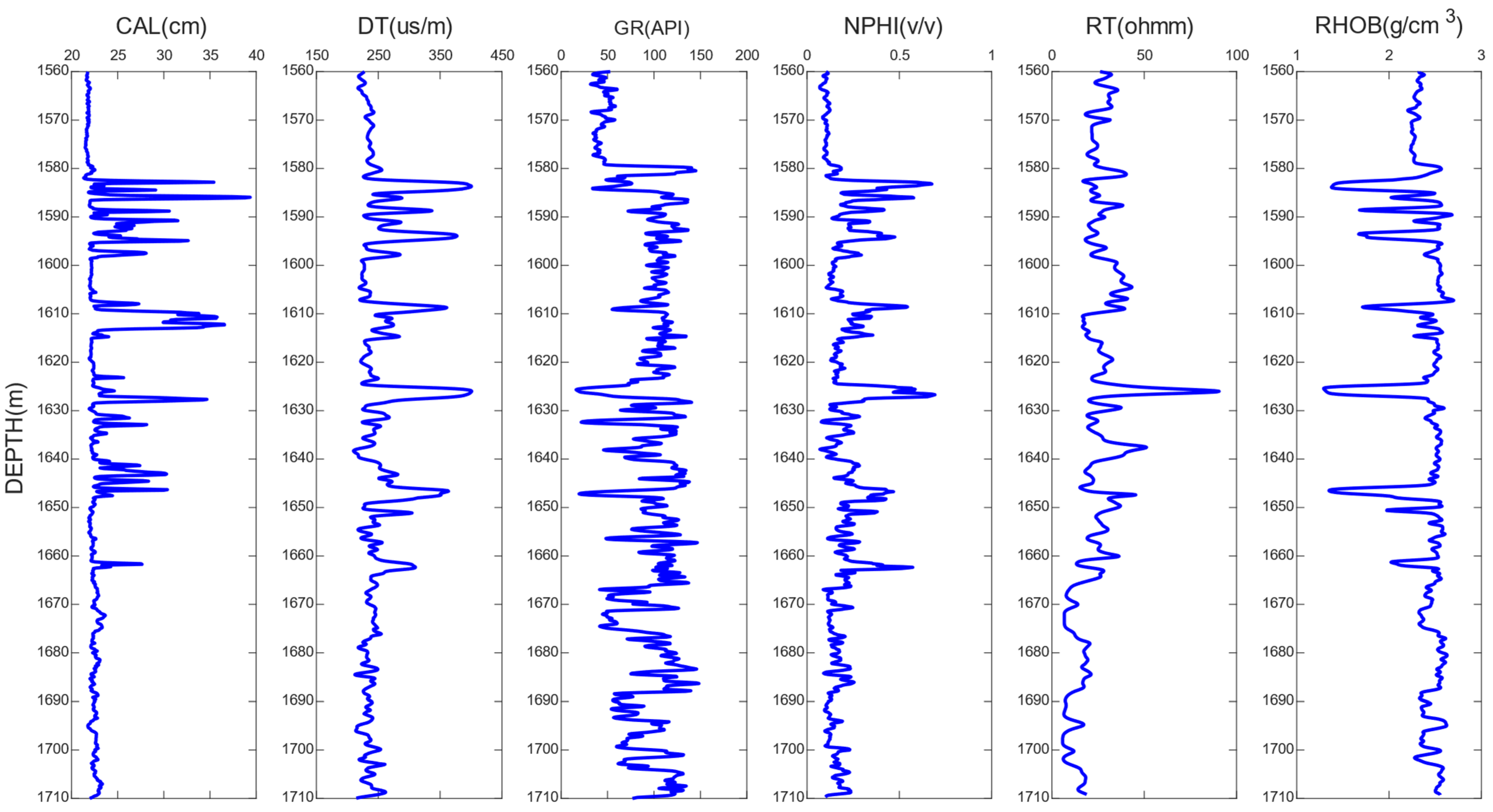
The exploration well that is studied is located in the Ordos basin, which is a craton basin formed by the superposition of multi-stage structures. To protect its privacy, the exploration well is labeled as well A. Figure 9 displays the log graph for well A. The response of the logging data provides a thorough representation of the associated subsurface formation’s lithology, physical characteristics, electrical characteristics, and oil–gas characteristics.

4.3. Model Parameter Setting

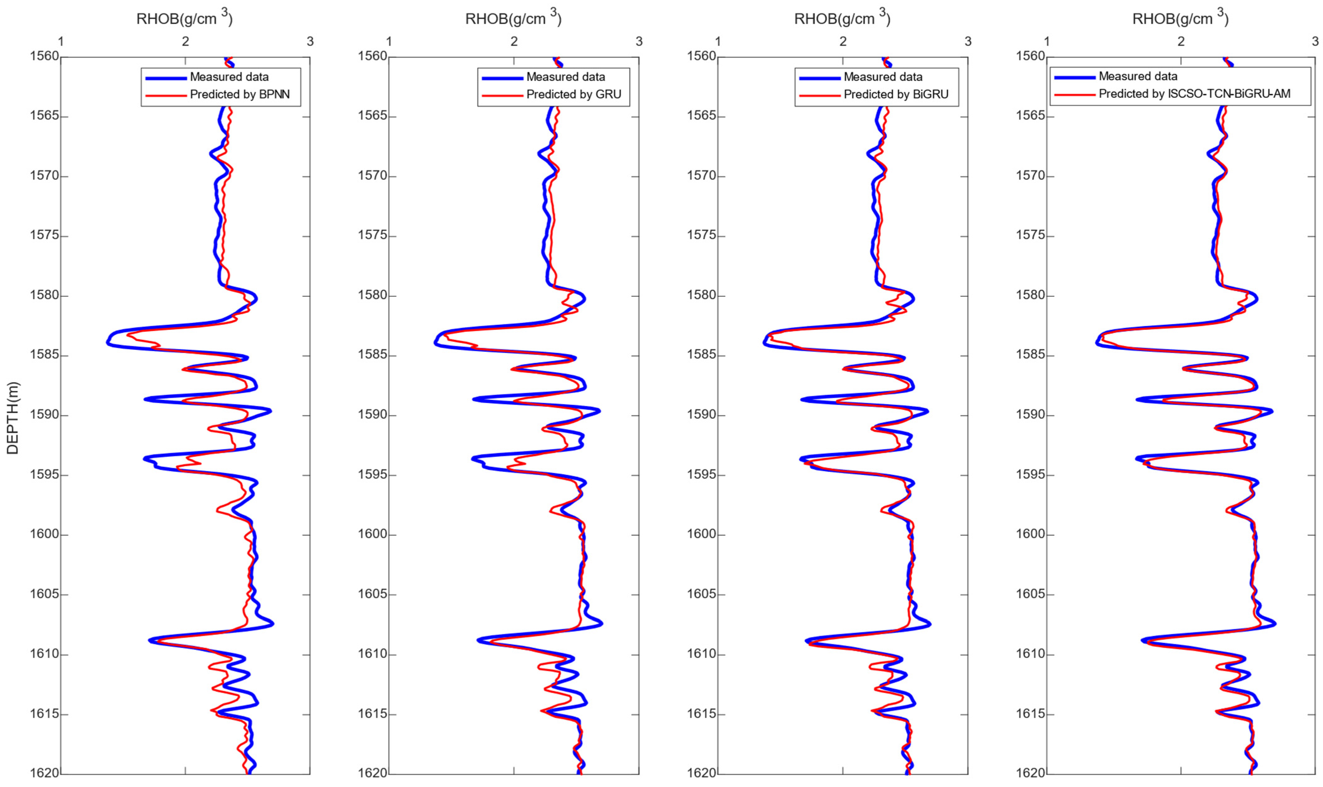
Logging data at depths ranging from 1621 to 1710 m are used as the training data to build the models, including the back propagation neural network (BPNN) [20], GRU [21], BiGRU-AM [22], and ISCSO-TCN-BiGRU-AM. The training models take six parameters as inputs: DEPTH, CAL, NPHI, GR, DT, and RT. Furthermore, the output parameter is RHOB. The “missing” RHOB at depths between 1560 and 1620 m can be anticipated using the learned models.
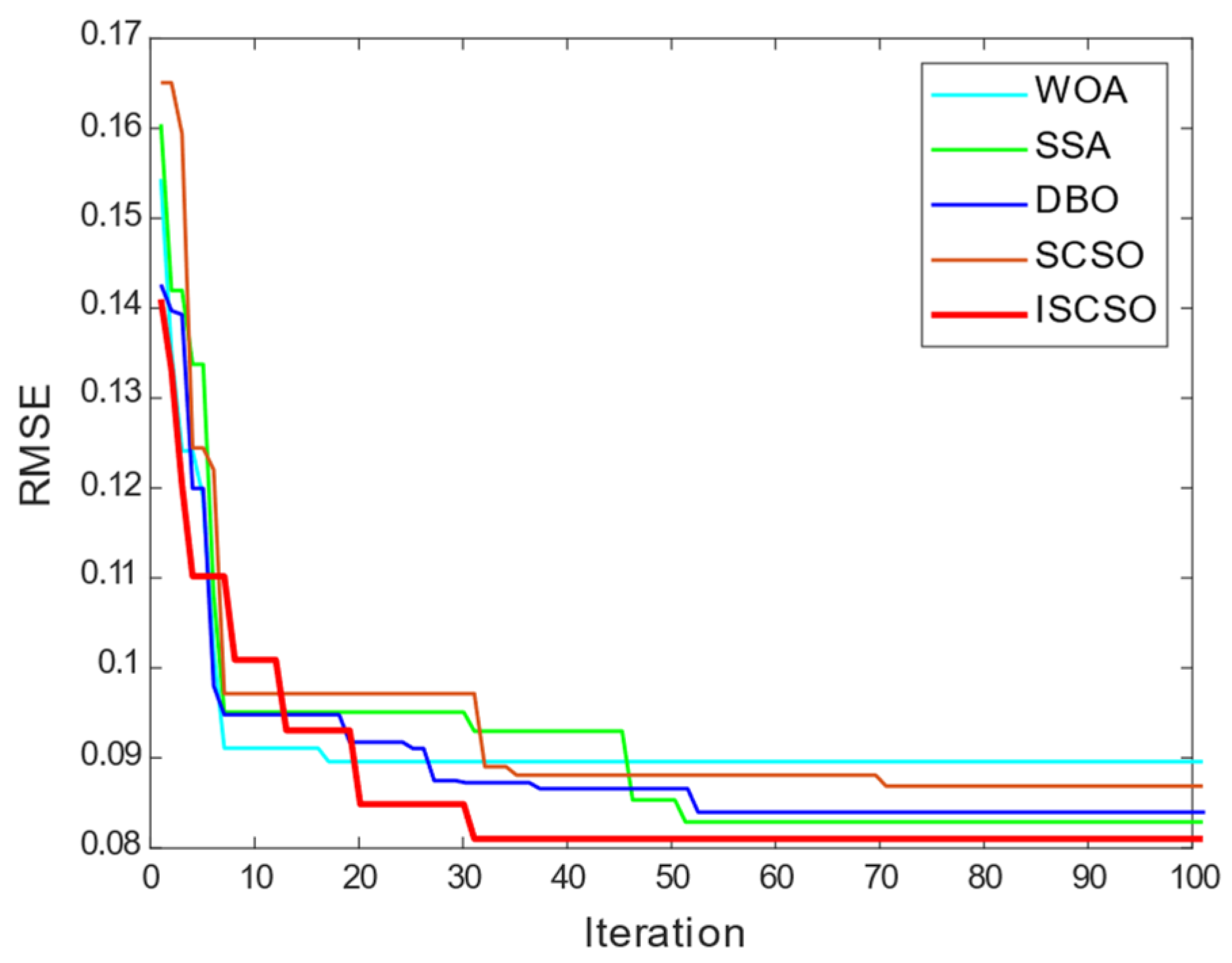
The TCN-BiGRU-AM is optimized by the ISCSO. The goal of the optimization procedure is to find the optimal combination of hyperparameters with the best fitness value. In this paper, the RMSE is used as the fitness evaluation index. The search range of relevant parameters is restricted to avoid a large search space, impacting the optimization efficiency. Specifically, the initial learning rate is in the range of [ 10 4 ,   10 3 ] , and the optimal value is 0.002 . The number of nodes in the hidden layer is in the range of [ 10 ,   100 ] , and the optimal value is 50 . The number of filters is in the range of 2 ,   60 , and the optimal value is 54 . The L2 regularization coefficient is in the range of [ 10 8 , 10 2 ] , and the optimal value is 0.004 .
Figure 10 displays the fitness decline rate of the TCN-BiGRU-AM in the training phase. It is evident that the ISCSO converges faster than the competing algorithms. Furthermore, the ISCSO’s final error is less than that of the competing optimization methods, further demonstrating its superiority.

4.4. Analysis of Prediction Results

Table 3 displays the prediction outcomes for the competing models and the ISCSO-TCN-BiGRU-AM. The mean absolute error (MAE) is expressed as follows:
M A E = 1 N i = 1 N y k y ^ k
where y k and y ^ k are the real and predicted values, respectively.
As can be seen in Table 3, the predicted performance of deep learning models based on a recurrent neural network (BiGRU, BiGRU-AM, and ISCSO-TCN-BiGRU-AM) is better than that of the ordinary neural network model (BPNN). Furthermore, the ISCSO-TCN-BiGRU-AM is the best. Compared to the competing models, the ISCSO-TCN-BiGRU-AM requires more time to complete tasks. However, the ISCSO-TCN-BiGRU-AM has the lowest prediction error of all the methods. Comparatively, the ISCSO-TCN-BiGRU-AM only requires a slight amount of extra time and has the highest accuracy. After comprehensive consideration, it is concluded that the ISCSO-TCN-BiGRU-AM has more practical application ability than the competing methods.
The estimated RHOB at depths ranging from 1560 to 1620 m is shown in Figure 11. When the logging curves change smoothly, all models achieve good reconstruction results. When the local logging curve mutation (1582–1587 m, 1593–1596 m) occurs, the predicted values of the deep learning models based on a recurrent neural network (BiGRU, BiGRU-AM, and ISCSO-TCN-BiGRU-AM) are closer to the real data than the value predicted by the BPNN. Furthermore, the ISCSO-TCN-BiGRU-AM has the best predictive performance. The BPNN establishes the nonlinear mapping relationship of the same interval and does not consider the characteristics of logging data changing with the depth. Therefore, when there is a sudden change in the logging data, the reconstruction results based on the BPNN will have a large deviation. The TCN-BiGRU-AM belongs to a combined dynamic deep learning model. It primarily takes advantages of the benefits of TCN, BiGRU, and AM in processing timeseries data and the optimization ability of the ISCSO. A TCN is used to eliminate redundant features since this is an efficient way to extract hidden information and temporal correlations from features. A BiGRU may also retrieve the contextual correlation of the features. With AM, the long-distance relationships between characteristics are more effectively captured. ISCSO is used to optimize the hyperparameters of TCN-BiGRU-AM. These not only enable the ISCSO-TCN-BiGRU-AM to make full use of the nonlinear characteristics, but also to learn the characteristics of logging data changing with depth. Therefore, a TCN-BiGRU-AM network model has higher stability and accuracy in logging reconstruction than the competing models.
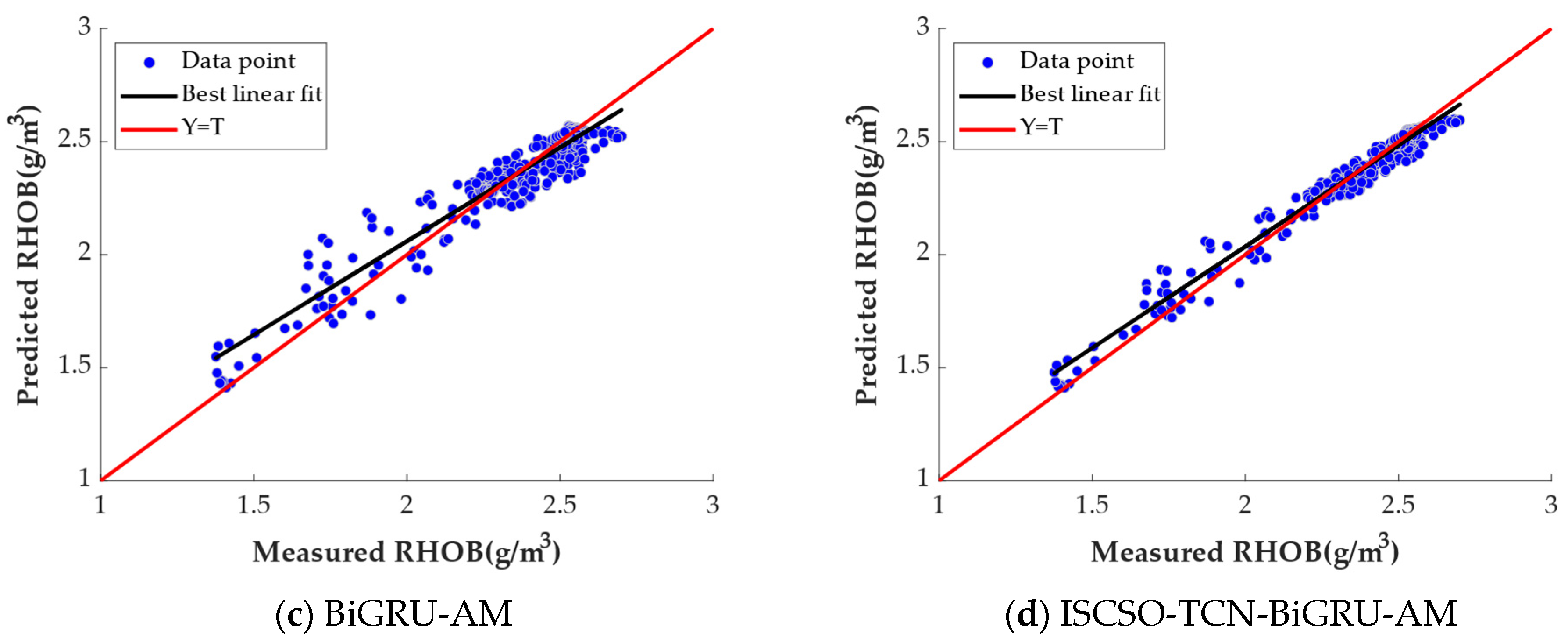
The cross-plots of the real RHOB versus the RHOB predicted by the trained models are displayed in Figure 12.
It can be demonstrated that, compared to the competing models, the predicted RHOB of the ISCSO-TCN-BiGRU-AM is more in line with the real RHOB. To sum up, the ISCSO-TCN-BiGRU-AM exhibits a strong predictive ability for both the overall and local sudden changes in logging curves, adequately illustrating its benefits in anticipating missing logging data.

5. Conclusions

A combined model named ISCSO-TCN-BiGRU-AM is proposed for well logging reconstruction, and it is verified by the logging data set from the Ordos Basin. The following conclusions can be obtained:
(1)
The ISCSO with variable spiral strategy and sparrow warning mechanism enhances population diversity, boosts the average search efficiency, and lessens the tendency to quickly settle into the local optimum during the search process.
(2)
The TCN-BiGRU-AM integrates the network architectures of a TCN and BiGRU-AM. This hybrid architecture can not only deal with complex time dependence but can also improve processing adaptability to the dynamic characteristics of the time series.
(3)
The ISCSO can enhance the prediction performance by optimizing the hyperparameters. Compared with the competing models, the ISCSO-TCN-BiGRU-AM can more effectively make an accurate prediction. It has high utilization and practical application values.
In conclusion, the ISCSO-TCN-BiGRU-AM has excellent prediction performance. It is capable of meeting practical engineering demands. Of course, it is limited by the high model complexity and big model size caused by the enormous number of factors in the proposed method, making it challenging to implement on mobile terminal devices. Our next work will concentrate on lightweight networks with high accuracy.

Author Contributions

Conceptualization, G.W.; methodology, G.W.; software, H.T.; validation, L.Q. and Y.C.; formal analysis, H.Y.; investigation, L.Q.; resources, Y.C.; data curation, Y.C.; writing—original draft preparation, L.Q.; writing—review and editing, L.Q.; visualization, L.Q.; supervision, L.Q.; project administration, L.Q.; funding acquisition, K.X. All authors have read and agreed to the published version of the manuscript.

Funding

This research was funded by State Key Laboratory of Nuclear Resources and Environment Joint Innovation Fund “Research on Sandstone type Uranium Reservoir Logging Identification Method Based on Machine Learning” (2022NRE-LH-18).

Data Availability Statement

The data presented in this study are available upon request from the corresponding author. The data are not publicly available due to the confidentiality requirements of the data provider.

Conflicts of Interest

The authors declare no conflicts of interest.

References

  1. Sarhan, M.A. Geophysical assessment and hydrocarbon potential of the Cenomanian Bahariya reservoir in the Abu Gharadig Field, Western Desert, Egypt. J. Pet. Explor. Prod. Technol. 2021, 11, 3963–3993. [Google Scholar] [CrossRef]
  2. Qiao, L.; He, N.; Cui, Y.; Zhu, J.; Xiao, K. Reservoir Porosity Prediction Based on BiLSTM-AM Optimized by Improved Pelican Optimization Algorithm. Energies 2024, 17, 1479. [Google Scholar] [CrossRef]
  3. Qiao, L.; Cui, Y.; Jia, Z.; Xiao, K.; Su, H. Missing Well Logs Prediction Based on Hybrid Kernel Extreme Learning Machine Optimized by Bayesian Optimization. Appl. Sci. 2022, 12, 7838. [Google Scholar] [CrossRef]
  4. Farouk, S.; Sen, S.; Belal, N.; Omran, M.A.; Assal, E.M.; Sarhan, M.A. Assessment of the petrophysical properties and hydrocarbon potential of the lower Miocene Nukhul formation in the Abu Rudeis-Sidri Field, Gulf of Suez Basin, Egypt. Geomech. Geophys. Geo-Energy Geo-Resour. 2021, 9, 36. [Google Scholar] [CrossRef]
  5. Smith, J.H. A Method for Calculating Pseudo Sonics from E-Logs in a Clastic Geologic Setting. GCAGS Trans. 2007, 57, 1–4. [Google Scholar]
  6. Wang, J.; Liang, L.; Qiang, D.; Tian, P.; Tan, W. Research and application of reconstructing logging curve based on multi-source regression model. Lithol. Reserv. 2016, 28, 113–120. [Google Scholar]
  7. Liao, H.M. Multivariate regression method for correcting the influence of expanding diameter on acoustic curve of density curve. Geophys. Geochem. Explor. 2014, 38, 174–179. [Google Scholar]
  8. He, X.H.; Li, K.S.; Xu, J.C.; Fu, M.Y.; Yang, Y.F.; Sun, J.Q. Application of Log Lithofacies Classification Model Based on Clustering-Support Vector Classification Method. Well Logging Technol. 2023, 47, 129–137. [Google Scholar]
  9. Ramachandram, D.; Taylor, G.W. Deep Multimodal Learning: A Survey on Recent Advances and Trends. IEEE Signal Process. Mag. 2017, 34, 96–108. [Google Scholar] [CrossRef]
  10. Rolon, L.; Mohaghegh, S.D.; Ameri, S. Using artificial neural networks to generate synthetic well logs. J. Nat. Gas Sci. Eng. 2009, 1, 118–133. [Google Scholar] [CrossRef]
  11. Duan, Y.X.; Xu, D.S.; Sun, Q.F.; Li, Y. Research and Application on DBN for Well Log Interpretation. J. Appl. Sci. 2018, 36, 689–697. [Google Scholar]
  12. Rahman, A.; Srikumar, V.; Smith, A.D. Predicting electricity consumption for commercial and residential buildings using deep recurrent neural networks. Appl. Energy 2018, 212, 372–385. [Google Scholar] [CrossRef]
  13. Zhang, Y.; Ai, Q.; Lin, L.; Yuan, S.; Li, Z. A very short-term load forecasting method based on deep LSTM RNN at zone leve. Power Syst. Technol. 2019, 43, 1884–1892. [Google Scholar]
  14. Niu, D.; Yu, M.; Sun, L.J.; Gao, T.; Wang, K.K. Short-term multi-energy load forecasting for integrated energy systems based on CNN-BiGRU optimized by attention mechanism. Appl. Energy 2022, 313, 118801. [Google Scholar] [CrossRef]
  15. Yang, W.B.; Xia, K.W.; Fan, S.R. Oil Logging Reservoir Recognition Based on TCN and SA-BiLSTM Deep Learning Method. Eng. Appl. Artif. Intell. 2023, 121, 105950. [Google Scholar] [CrossRef]
  16. Seyyedabbasi, A.; Kiani, F. Sand Cat swarm optimization: A nature-inspired algorithm to solve global optimization problems. Eng. Comput. 2022, 39, 2627–2651. [Google Scholar] [CrossRef]
  17. Xue, J.; Shen, B. Dung beetle optimizer: A new meta-heuristic algorithm for global optimization. J. Supercomput. 2022, 79, 7305–7336. [Google Scholar] [CrossRef]
  18. Xue, J.; Shen, B. A novel swarm intelligence optimization approach: Sparrow search algorithm. Syst. Sci. Control. Eng. 2020, 8, 22–34. [Google Scholar] [CrossRef]
  19. Seyedali, M.; Andrew, L. The Whale Optimization Algorithm. Adv. Eng. Softw. 2016, 95, 51–67. [Google Scholar]
  20. Vaferi, B.; Eslamloueyan, R.; Ayatollahi, S. Automatic recognition of oil reservoir models from well testing data by using multi-layer perceptron networks. J. Pet. Sci. Eng. 2011, 77, 254–262. [Google Scholar] [CrossRef]
  21. Zeng, L.; Ren, W.; Shan, L. Attention-based bidirectional gated recurrent unit neural networks for well logs prediction and lithology identification. Neurocomputing 2020, 414, 153–171. [Google Scholar] [CrossRef]
  22. Bensoltane, R.; Zaki, T. Combining BERT with TCN-BiGRU for enhancing Arabic aspect category detection. J. Intell. Fuzzy Syst. 2023, 44, 4123–4136. [Google Scholar] [CrossRef]
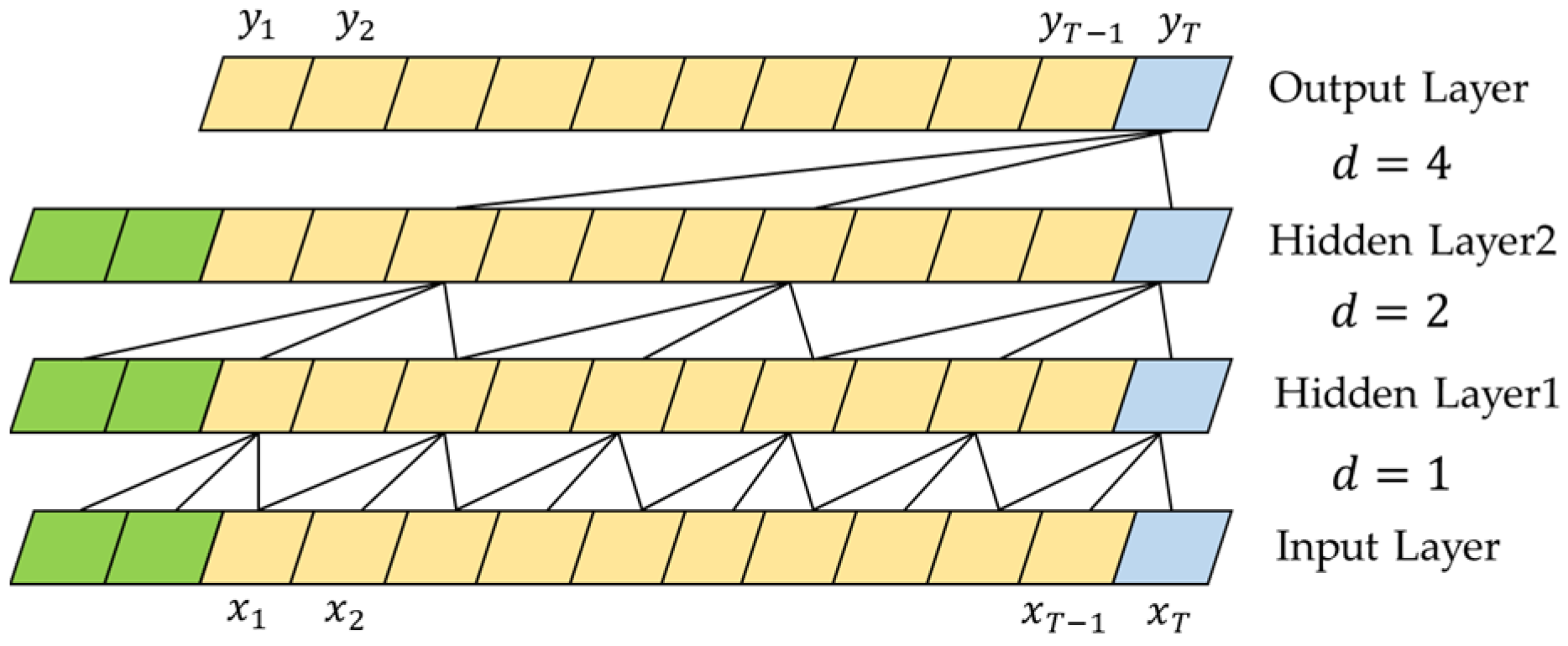
Figure 1. Architecture of dilated causal convolution.
Energies 17 02710 g001
Figure 2. Residual network of TCN.
Energies 17 02710 g002
Figure 3. Framework of GRU.
Energies 17 02710 g003
Figure 4. Framework of BiGRU.
Energies 17 02710 g004
Figure 5. Framework of AM.
Energies 17 02710 g005
Figure 6. Framework of TCN-BiGRU-AM.
Energies 17 02710 g006
Figure 7. Flowchart of ISCSO.
Energies 17 02710 g007
Figure 8. Convergence curves of ISCSO and competing algorithms.
Energies 17 02710 g008
Figure 9. Logging graph of well A.
Energies 17 02710 g009
Figure 10. Fitness reduction rate of ISCSO and competing algorithms.
Energies 17 02710 g010
Figure 11. Logging diagrams of the estimated RHOB by ISCSO-TCN-BiGRU-AM and the competing models.
Energies 17 02710 g011
Figure 12. Prediction comparison between ISCSO-TCN-BiGRU-AM and competing models.
Energies 17 02710 g012aEnergies 17 02710 g012b
Table 1. The results of the ISCSO and the competing algorithms on CEC–2022 functions. The best values are bolded, and the standard deviation is indicated with parenthesis.
FunctionISCSO SCSO DBOSSAWOA
F13.00 × 1022.08 × 1037.69 × 1024.99 × 1031.14 × 103
(1.55 × 10²)(2.33 × 10³)(9.13 × 10²)(2.45 × 10³)(5.45 × 10²)
F24.12 × 1024.41 × 1024.34 × 1024.46 × 1024.64 × 102
(2.10 × 101)(3.43 × 101)(3.43 × 101)(3.02 × 101)(4.45 × 101)
F36.18 × 1026.23 × 1026.21 × 1026.20 × 1026.41 × 102
(9.06 × 100)(9.66 × 100)(1.15 × 101)(1.04 × 101)(1.30 × 101)
F48.20 × 1028.27 × 1028.23 × 1028.48 × 1028.26 × 102
(7.06 × 100)(6.78 × 100)(5.19 × 100)(6.6 × 100)(9.18 × 100)
F59.88 × 1021.11 × 1031.10 × 1039.79 × 1021.45 × 103
(2.85 × 101)(1.25 × 10²)(1.10 × 10²)(4.80 × 101)(1.76 × 10²)
F63.15 × 1034.54 × 1033.02 × 1035.76 × 1047.70 × 103
(1.56 × 10³)(2.15 × 10³)(1.82 × 10³)(3.51 × 10⁴)(6.59 × 10³)
F72.01 × 1032.05 × 1032.04 × 1032.08 × 1032.08 × 103)
(1.38 × 101)(2.97 × 101)(1.55 × 101)(3.38 × 101)(2.92 × 101)
F82.21 × 1032.23 × 1032.22 × 1032.26 × 1032.24 × 103
(3.66 × 101)(5.90 × 100)(8.34 × 100)(3.27 × 101)(1.39 × 101)
F92.52 × 1032.58 × 1032.55 × 1032.65 × 1032.61 × 103
(3.05 × 101)(4.28 × 101)(3.89 × 101)(4.68 × 101)(4.32 × 101)
F102.51 × 1032.56 × 1032.56 × 1032.63 × 1032.59 × 103
(3.09 × 101)(6.68 × 101)(6.33 × 101)(4.45 × 101)(6.86 × 101)
F112.82 × 1032.80 × 1032.83 × 1033.22 × 1032.84 × 103
(1.16 × 10²)(1.54 × 10²)(1.87 × 10²)(2.24 × 10²)(1.32 × 10²)
F122.87 × 1032.87 × 1032.87 × 1032.88 × 1032.95 × 103
(7.06 × 100)(1.69 × 101)(8.01 × 100)(2.06 × 101)(8.41 × 101)
Table 2. The test results of the ISCSO and the competing algorithms. The bold text denotes that the ISCSO is similar to the competing algorithms, where p > 0.05.
FunctionISCSO vs. SCSOISCSO vs. DBOISCSO vs. SSAISCSO vs. WOA
F13.02 × 10−113.02 × 10−113.02 × 10−113.02 × 10⁻¹¹
F21.77 × 10−47.23 × 10−33.58 × 10−81.84 × 10⁻⁶
F31.41 × 10−35.30 × 10−37.24 × 10−32.15 × 10⁻⁶
F41.98 × 10−33.91 × 10−34.44 × 10−42.17 × 10⁻³
F52.78 × 10−73.26 × 10−71.07 × 10−93.04 × 10⁻¹
F62.50 × 10−38.24 × 10−33.34 × 10−111.11 × 10⁻⁶
F75.79 × 10−36.97 × 10−31.12 × 10−37.98 × 10⁻³
F84.35 × 10−53.78 × 10−38.35 × 10−88.20 × 10⁻⁷
F92.75 × 10−52.75 × 10−55.31 × 10−71.21 × 10⁻⁵
F101.29 × 10−61.49 × 10−49.92 × 10−115.07 × 10⁻¹⁰
F116.18 × 10−22.61 × 10−11.49 × 10−82.61 × 10⁻¹
F124.92 × 10−12.17 × 10−15.60 × 10−76.72 × 10⁻¹⁰
Table 3. Comparison of prediction results.
ModelRMSEMAETime (s)
BPNN0.10200.081515.6341
GRU0.09560.071225.1322
BiGRU-AM0.07550.057431.2581
ISCSO-TCN-BiGRU-AM0.06140.045742.2412
Disclaimer/Publisher’s Note: The statements, opinions and data contained in all publications are solely those of the individual author(s) and contributor(s) and not of MDPI and/or the editor(s). MDPI and/or the editor(s) disclaim responsibility for any injury to people or property resulting from any ideas, methods, instructions or products referred to in the content.