1. Introduction
The rapid advancement in science and technology, along with the continuous enhancement in living standards, has gradually depleted traditional energy sources over time. Consequently, reliance on traditional energy has shifted towards cleaner, more sustainable forms of energy consumption [
1]. This shift has led to an increase in the number of connections between power sources and loads, complicating the system’s topology. This complexity introduces multi-directional line current flows, increasing the risk of line current loops, unbalance, and susceptibility to short-circuit faults. When such faults arise, the remaining distributed power sources may inadvertently sustain power in the fault area, creating an “islanding effect”. This not only endangers the safety of maintenance personnel but also threatens the normal functioning of equipment [
2]. Therefore, the precise detection of fault locations and types, along with the timely implementation of protective measures, has become a critical area of research. Fault detection methods play a crucial role in selecting appropriate line protection strategies.
The traditional power transmission network is characterized by its unidirectional current flow and susceptibility to short-circuit faults [
3]. Commonly, techniques such as thresholding or a logical analysis based on distribution automation data are employed to identify the specific type and location of faults. The authors of [
4] suggested extracting electrical signal features using a dual-threshold fault sample support vector data (SVDD) approach, combined with wavelet packet energy features and Spearman correlation coefficients, to enable precise feature extraction across multiple signal types. Additionally, a modified SVDD fault warning algorithm was introduced to address the delays and accuracy issues associated with traditional SVDD in fault judgment. This algorithm adjusts the original SVDD boundaries to create a double-layer boundary, subdividing the hypersphere space into three zones, thereby enhancing sensitivity to fault samples. Ref. [
5] introduced the concept of fault-location observability and a novel scheme for fault localization in transmission networks, utilizing synchronized phasor measurement units (PMUs). This scheme minimized the number of PMUs required, ensuring their optimal placement within the network to achieve accurate fault localization. It incorporated a fault-localization algorithm and a fault-side selector to enhance precision. In Ref. [
6], addressing the limitations of traditional methods such as low sampling rates and inadequate sensitivity, a new approach for a precise localization of ground faults in distribution lines was proposed. This method leverages time-domain synchronization information for calculation. The data were first preprocessed through low-frequency time-domain signal reconstruction and cubic spline interpolation. Voltage and current constraints at the fault point were then used to establish various location criteria for the fault current, allowing for accurate fault location at lower sampling rates by computing the differences in fault currents at selected calculation points. A phasor measurement unit (PMU)-based method for fault localization and classification was detailed in [
7]. By introducing virtual buses, this method pinpointed the exact fault location along the line rather than merely identifying the nearest bus. Following fault localization, a generalized fault model (GFM) was applied to classify the fault type by solving a minimization problem, which calculated the fault impedance. This model could distinguish whether the fault occurred on a branch line or the main feeder without needing an additional PMU at the branch line’s end.
However, conventional transmission network switches typically prolong their reset frequency. Intermittently distributed power sources can cause frequent hourly reconfigurations of traditional distribution network switches [
8]. This scenario poses a significant challenge to conventional line protection monitoring methods and is ill suited for the contemporary power system architecture, which incorporates multiple microgrids (MGs). As a result, the emphasis on line fault detection in modern power systems has increasingly shifted to studying MGs that include multiple distributed power sources. This shift underscores the need for developing fault detection methods that are adaptable and effective within the complex dynamics of MG environments. The artificial intelligence model can be adjusted and expanded according to different application requirements and integrated into the existing system, adapting to various sizes and types of MGs and improving the system’s detection capability and intelligence level. Meanwhile, through automated fault detection and diagnoses, it provides a fault cause analysis and preventive maintenance recommendations to support comprehensive management and maintenance of the system, which reduces the dependence on manual detection and maintenance and lowers operation and maintenance costs.
Currently, the advantages of AI techniques, including a data analysis and autonomous learning, such as Extreme Gradient Boosting (XGBoost), a Gradient Boosting Decision Tree (GBDT), a neural network (NN), and a Support Vector Machine (SVM), are increasingly recognized in various fields [
9,
10,
11,
12]. In the realm of MG management, the reliance of artificial intelligence on operational data means that changes in the MG structure have minimal impact on the AI’s ability to perform classification, prediction, and identification tasks. This resilience has led to the growing application of AI in MG line fault monitoring [
13]. For instance, ref. [
14] outlined an intelligent fault detection scheme for MGs that utilizes wavelet transforms and deep neural networks. This scheme was designed to quickly provide crucial information about fault type, phase, and location, aiding MG protection and service restoration. In this approach, branch current measurements collected by protection relays are preprocessed using a discrete wavelet transform to extract statistical features. These features are then input into a deep neural network, which is trained to develop fault information. Ref. [
15] presented a mesh-structured fault detection and identification method for low-voltage DC MGs, employing a graph convolutional network (GCN). This method leveraged explicit spatial information from the network topology and measurement data for more effective fault identification, even in the presence of noise and erroneous data. The adjacency matrix for the GCN was developed by treating the network topology as an intrinsic graph. Further enhancing MG fault detection, ref. [
16] proposed a differential relay scheme based on a data mining model. This scheme provided a fixed-setting, fast, and reliable method for the accurate detection and classification of faults. It utilized three-phase current signals from both ends of the distribution line to calculate differential current phases, incorporating distributed generation (DG) in the fault model. A deep neural network (DNN)-based data mining model was then constructed using a dataset generated from MG faults and changes in operating conditions, which included various fault types, locations, fault resistances, and variations in DG penetration rates and operating modes. In another innovative approach, ref. [
17] described an MG fault diagnosis method using a whale algorithm-optimized Extreme Learning Machine (ELM). Initially, the three-phase fault voltage was analyzed using the wavelet packet decomposition method, and a feature vector consisting of wavelet packet energy entropy was calculated. The whale algorithm was then employed to optimize the ELM’s input weights and hidden layer neuron thresholds. This optimization addressed the issue of random initialization potentially affecting network performance, thereby enhancing the learning speed and generalization ability of the network, which is crucial for global optimization.
The AI techniques referenced in the literature have shown significant benefits in fault detection. However, these models depend on large datasets and involve complex computational processes. This requirement makes the fault detection process computationally intensive, particularly in MG structures that feature numerous branched circuits with distributed power sources. Additionally, the complexity of these AI model designs can be a hindrance, as it affects both the internal architecture of the models and their operational calculations. This complexity may not only limit the models’ efficiency but also complicate their implementation and scalability within diverse MG environments. Such challenges necessitate the development of more streamlined AI models that maintain high accuracy while reducing computational demands.
Additionally, relying solely on neural networks or machine learning algorithms to learn data features from a large volume of data can lead to challenges such as overfitting during the data learning and training process. This issue not only increases the complexity and computational demands of model operations but also significantly augments the operational workload. To address these challenges, it is essential to integrate a robust classification function into the fault detection model. This function would pre-categorize the data, thereby enhancing the model’s efficiency by directing the learning process towards more relevant features and reducing the likelihood of overfitting. Implementing such a function would streamline operations and improve the accuracy and reliability of fault detection in complex MG systems.
To overcome the limitations previously highlighted, this study introduces a novel MG fault detection method that employs a LightGBM-NN framework, integrating a Shapley value analysis and a bagging-integrated learning algorithm. This method is rooted in the gradient boosting framework, renowned for its robust classification capabilities, rapid processing speeds, and minimal memory requirements. The approach starts by selecting fault voltage and voltage fundamentals at the measurement point as feature indices. It further extracts additional fault feature samples, such as voltage peaks across different frequency bands, phase-to-phase voltage differences, and the sixth harmonic component. Using these features, the LightGBM model classifies MG lines’ normal and fault operation data. To enhance the robustness of the model, a bagging-integrated learning algorithm is employed. This involves training a base model independently for each training subsample set, followed by a parallel combination of these models. The outputs from all base models are then averaged and fed into a neural network, facilitating active learning of data features. Lastly, the Shapley value method is incorporated into the combined model to quantify the contribution of each feature to the fault prediction when different branches of the MG experience faults. This aids in identifying the most influential features and visualizing the decision-making process in fault diagnoses. It also supports the future collection of feature data from various MG branches, mitigating the issue of the high computational load typical of conventional models. At the same time, feature interpretation methods are often very sensitive to changes in the data. The integrating effect of the bagging method averages the predictions of multiple models, resulting in a more stable and reliable interpretation of Shapley values. This integrated approach improves the accuracy of fault detection and provides valuable insights for ongoing research on MG fault detection while ensuring transparency and interpretability of the model outputs. This increased transparency enhances the trust of all stakeholders in the model’s decisions.
2. A Framework for Fault Detection in MG Systems
As an example, the simple MG system of
Figure 1 contains mainly DGs. In addition, the lines are labeled with measurement points (identified by numbers) and fault locations (labeled f
1).
In an MG with multiple distributed power sources, the occurrence of a short-circuit fault at a point such as f1 can lead the remaining sources to inadvertently create an islanding effect. This means that they continue to supply power to the faulted line, posing risks to both personnel and equipment involved in troubleshooting efforts. Moreover, the presence of numerous power electronic devices within the line exacerbates this situation when a short-circuit fault happens, as these devices generate specific harmonic components. These harmonics result in abnormal voltage harmonic performance at each measurement point during the fault. Analyzing the characteristic relationship between the voltage harmonic components at various measurement points and fault detection can provide deep insights into addressing such short-circuit issues. This analysis can form the basis of the characteristic sample set for the fault detection model. By using these harmonic profiles as key diagnostic features, the fault detection model can more accurately identify and localize faults, particularly by differentiating between normal operational harmonics and those indicative of fault conditions. This approach not only improves the accuracy of fault detection but also enhances the safety and reliability of MG operations.
In this paper, we employ voltage harmonic components at different measurement points as the target for analyzing MG faults. The comprehensive framework for our proposed LightGBM-NN combined model, which incorporates a bagging-integrated learning algorithm and Shapley value analysis, is demonstrated in
Figure 2. The implementation of this method is primarily divided into two stages, each comprising distinct modules aimed at enhancing the model’s effectiveness and transparency:
- (1)
Feature processing and screening using LightGBM-NN.
Module 1: LightGBM-Based Preliminary Data Feature Classification
This module involves loading raw MG operation data into internal memory to perform an initial high-quality feature screening. This stage is critical for identifying significant features that can effectively predict operational anomalies and faults in MG systems.
Module 2: Enhancement in the LightGBM Model Using the Bagging Method
Following the preliminary feature classification by LightGBM, the output is used as input to this module. Here, the data are divided into multiple training subsets. The diversity of feature classification is increased, and the risk of overfitting is mitigated by employing training set sampling and feature sampling techniques, which enrich the robustness of the LightGBM model.
Module 3: NN-Based Data Feature Training and Learning
In this module, the neural network (NN) takes the enhanced data features from the LightGBM model, refined by the bagging method, as input. Utilizing its active learning capabilities, the NN learns and trains on the MG operation data features, aiming to further refine fault detection accuracy.
- (2)
Model Result Evaluation Using Shapley Value.
Module 4: Shapley Value-Based Characteristic Contribution Calculation
This module calculates the contribution of data characteristics from different operational states of each MG branch to the prediction results of the LightGBM-NN combined model. The aim is to improve the transparency of the model’s fault detection and decision-making process. The results of the Shapley value analysis provide feedback for Module 1, enhancing the guidance for the subsequent data collection and visualization of characteristics specific to short-circuit faults across different lines of the grid. This feedback loop is essential for reducing the volume of data required for future collections and for refining the model’s predictive capabilities.
Building model development and evaluation processes through these modules ensures a systematic approach to enhancing fault detection in MGs. This method not only improves accuracy but also aids in understanding the underlying factors contributing to faults, thereby supporting more informed and effective decision-making in MG management.
3. LightGBM- and NN-Based Feature Processing Screening
3.1. Initial Feature Classification Based on LightGBM
The vast amount of operational data and the intensive computational demands across various branches of the MG result in prolonged model runtimes. This delay hinders the model’s ability to quickly detect operational faults. Consequently, there is an urgent need for an algorithmic model that not only saves time but also possesses robust computational capabilities for efficient fault classification.
Building on the traditional Gradient Boosting Decision Tree (GBDT) algorithm, LightGBM introduces several innovative enhancements. It extends the loss function through a second-order Taylor series and employs a Leaf-Wise decision tree growth strategy. This approach tightly controls the data expansion process, significantly reducing training time and memory consumption. Moreover, it markedly lowers the risk of overfitting and enhances the operational efficiency of the model [
18]. When handling large volumes of business data from microelectronic networks, LightGBM supports efficient parallel training. This capability allows it to swiftly process massive datasets while maintaining high classification accuracy and delivering clear classification outcomes. The basic steps for generating a strong classifier with LightGBM are as follows:
In the above equation, is the input feature quantity of the sample; is the true value of the sample.
Use
to fit one CART to obtain the
t class regression tree with the corresponding leaf node region
(
m = 1, 2, …,
M), where
M is the number of leaf nodes. Using greedy thinking to consider only local optimization, for each leaf node, solve to minimize the loss function, even if the best output value is
of the fitted leaf node.
where
is the fitted leaf node output value.
Let
be a simple parameterized function of the input variable in the region of leaf nodes, then the fitting function
of the decision tree is as follows:
Update to obtain a strong classifier for this round as
Let
be the initial model, which is iteratively combined by
T base models to obtain
, which is a strong classifier that can be obtained by the below equation.
Using the LightGBM internal classification regression tree as the base classifier, multiple individual decision tree classifiers are combined to obtain the final strong classifier through the cumulative model and stepwise boosting algorithm, which can improve the classification accuracy.
3.2. Model Improvement Based on Bagging Method
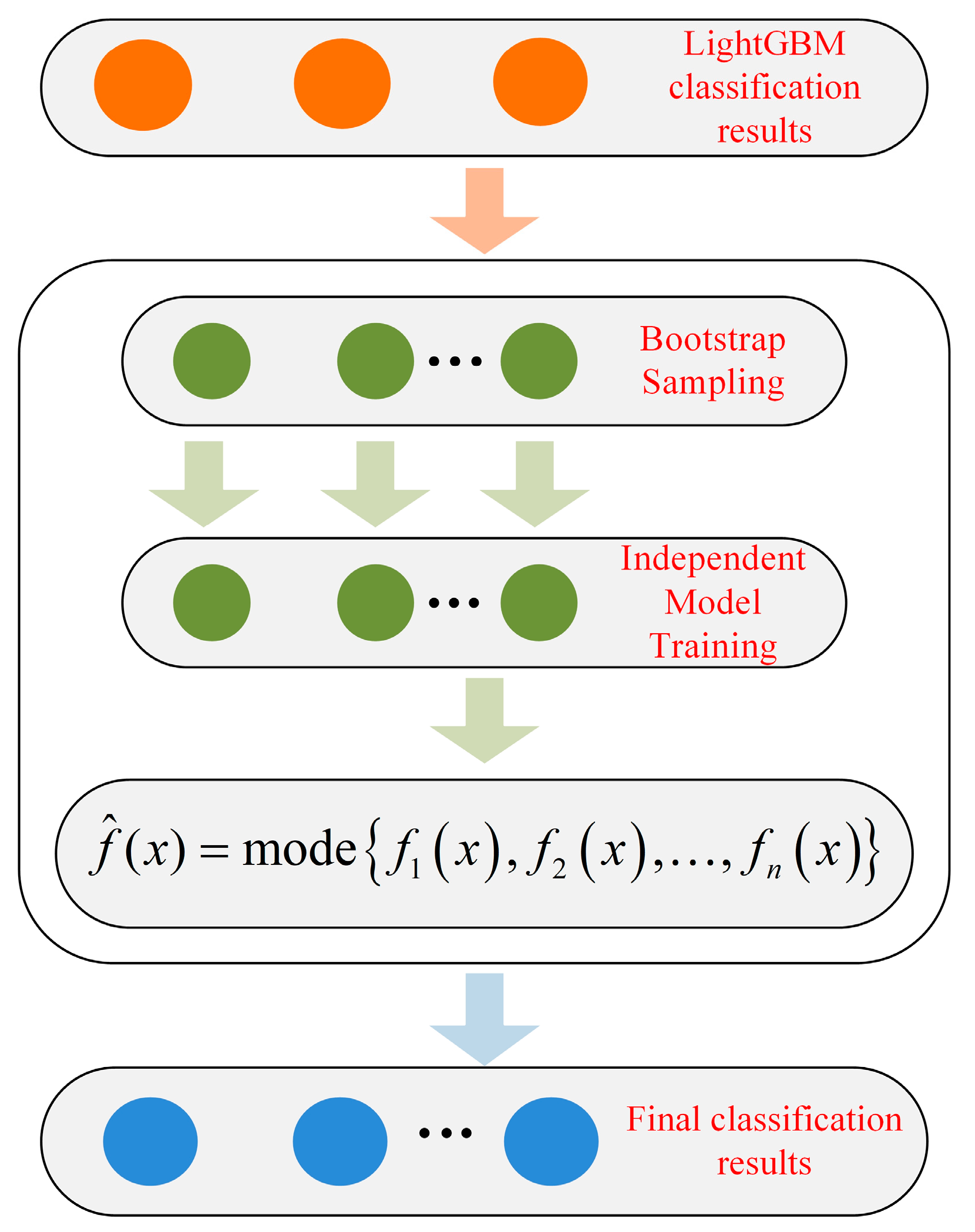
To enhance the classification stability and accuracy of LightGBM, the bagging method is introduced to smooth the results by merging multiple strong LightGBM classifier models. This approach helps reduce the models’ sensitivity to anomalies specific to individual samples. The bagging method, a parallel integrated learning algorithm, fundamentally involves training a base model on each training subset. These base models’ predictions are then combined to form a final prediction. The flowchart of this algorithm is illustrated in
Figure 3 [
19,
20]. This integration not only bolsters the robustness of the classification results but also ensures consistency across different data segments.
The basic implementation steps of the bagging method are shown in
Figure 3.
Introducing randomness in the sample construction module of the LightGBM model and parallel combination can improve the stability and accuracy of the LightGBM model, and at the same time reduce the model variance value. The preliminary classification results of LightGBM are composed into a training set D = {(x1, y1), (x2, y2), …, (xn, yn)}, where n is the number of samples in this training set.
Bootstrap Sampling: Perform putative back sampling from the training set D to extract n samples to form a new training set Dn. The process is repeated N times to generate N training datasets, D1, D2, …, DN.
Independent Model Training: For each dataset Db, a base learner fx(x) is trained independently.
Aggregation of Predictions: For a new input
x, each model
fn(
x) gives a prediction. These predictions are aggregated into a final prediction
. For the multi-terminal active distribution network fault detection problem, the majority voting system is used for result aggregation, and its mathematical expression is
where mode is a statistic of the value that occurs most often in a set of data.
3.3. NN-Based Data Feature Training Learning Phase
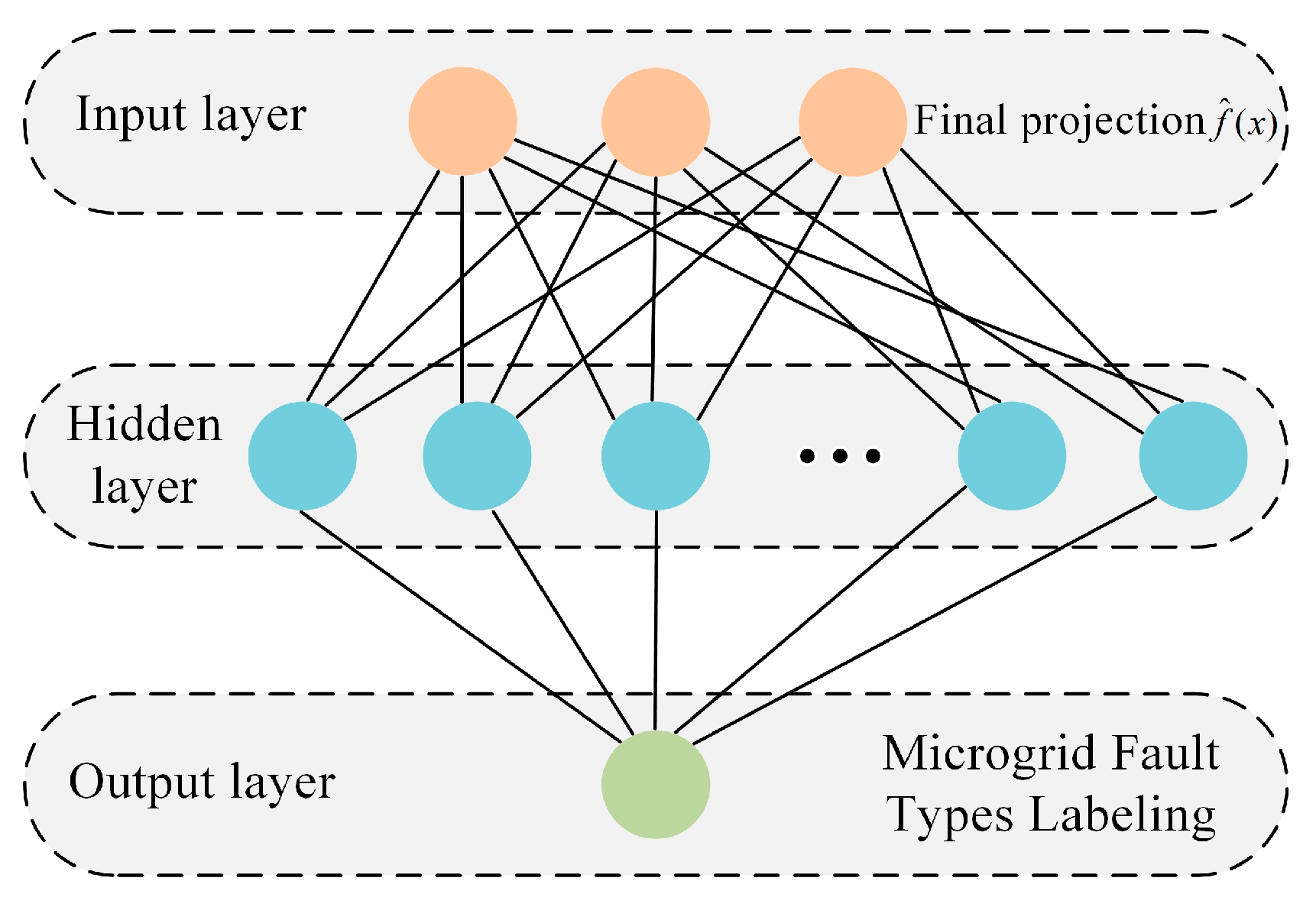
An NN, or neural network, is an architecture that excels in autonomously mining data features from a standard range for function estimation and approximation. A typical single-hidden-layer neural network comprises three main components: an input layer, a hidden layer, and an output layer. Each layer of neurons is fully connected to the subsequent layer [
21]. In this network, each neuron in the input layer represents predictions re-fined through the introduction of the bagging method within the LightGBM framework. The neurons in the output layer correspond to feature labels, which represent different fault types across various branches, as learned through the neural network’s training process. In this study, the neural network plays a crucial role in the combined model for fault localization at measurement points in multi-terminal active distribution networks and for the training and learning of fault-type data. This integration aids in assessing the future operational status of multi-terminal active distribution networks. The topology of this network is illustrated in
Figure 4.
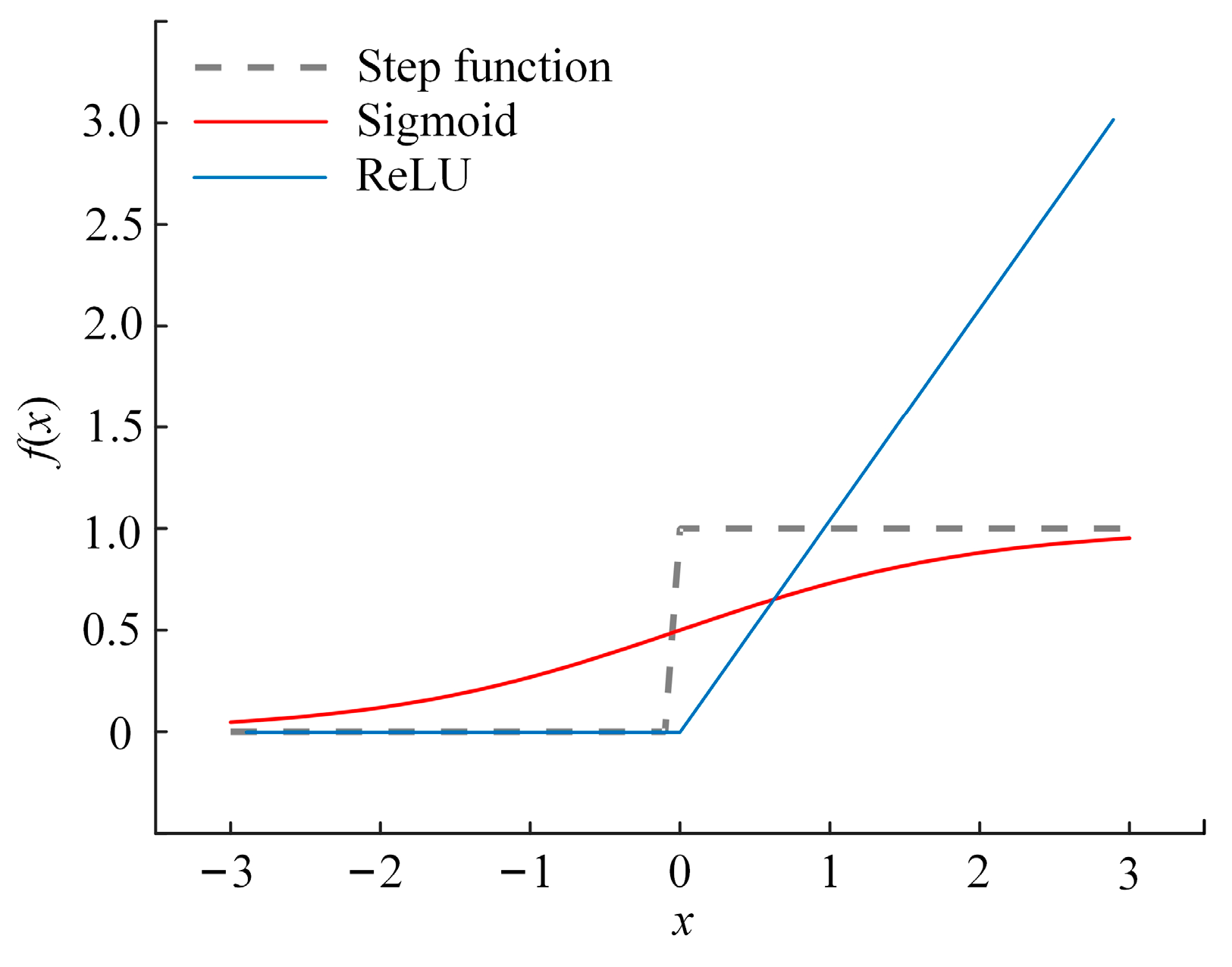
In a neural network, the output of each neuron is generated by the total input value it receives. Commonly used activation functions include the step function, sigmoid function, and ReLU (Rectified Linear Unit) function. These functions help determine the output at each neuron, effectively enabling the network to learn complex patterns and perform nonlinear modeling. The graphical representations of these activation functions are illustrated in
Figure 5.
Among them, the ReLU function can make the network have a certain sparsity and enhance the training speed; in this paper, the ReLU function is used as the activation function, and the expression is as follows [
22]:
3.4. Shapley Values Based on Cooperative Game Theory
Traditional machine learning fault detection models often rely on the superposition of complex nonlinear functions for decision-making, which can lead to poor interpretability. In practical fault detection tasks, these models may produce results without providing specific, actionable information about the feature quantities involved. This lack of transparency makes it difficult to understand and trust the model’s decisions, which can be a significant limitation in practical applications. Therefore, it is crucial to conduct a deep analysis of the model’s output decisions to enhance understanding and facilitate more effective implementation.
In this paper, a Shapley value analysis is introduced as an explanation framework after modeling, and the prediction of the example is explained by calculating the contribution of each feature to the model prediction, as shown in Equation (8).
In Equation (8),
n is the number of features;
ϕ0 is the baseline sample prediction; and
ϕj is the feature attribution Shapley value for feature
j. This is true in the case where the feature values are all present such that the sum of the feature attributions equals the output of the model to be explained, namely
. The marginal contribution of each feature is calculated for each feature of the model prediction using cooperative game theoretic value assignment. To obtain the Shapley values of features, the average of all feature contributions is taken to quantify the impact of each feature on the model prediction. That is, a weighted sum is performed on all combinations of feature values, expressed as Formulas (9) and (10).
In the above formulas, is the subset of features, is the number of features in the set , is the output value of the model under the combination of features, and is the set of features of all input samples.
Utilizing the principle of additivity of Shapley values, the tree’s Shapley values are reconstructed and processed using a weighted average. This approach is employed to further identify and predict potential faults in multi-terminal active distribution networks by training the neural network. The model processing involves calculating the contribution of each feature to the model’s prediction. This facilitates more efficient data computation and processing within the combined model, enhancing its learning efficiency. Additionally, by employing the Shapley value method to calculate the contribution of each feature, the model’s analysis process becomes visualized, making it more interpretable. The specific calculation formula is expressed as Formula (11).
3.5. Shapley Values Based on Cooperative Game Theory
To validate the recognition capability of the combined model on the existing dataset, and to ensure that the proportions of the individual categories in the generated training and test sets align with those in the original dataset, the performance evaluation is conducted using the following formulas. This approach guarantees that the model’s evaluation reflects its ability to generalize across different data distributions, maintaining the integrity and relevance of the test results.
where
ACC is the model measurement accuracy;
R is the model recall, which is the ratio of the number of samples correctly identified by the model as a positive class to the total number of samples that were actually positive;
TP is the number of samples correctly predicted by the model as a positive class;
FN is the number of samples where the model incorrectly predicted a positive class to be a negative class;
FP is the number of samples where the model incorrectly predicted a negative class to be a positive class; and
TN is the number of samples correctly predicted by the model to be a negative class.
4. Simulations and Results
In this study, a simulation model of an IEEE 33-node MG is constructed using Matlab/Simulink software, as depicted in
Figure 6. Within the MG, the different branch measurement points—specifically numbered 9, 22, 24, and 33—correspond to four distributed power sources. Measurement point 22 features a grid-connected photovoltaic (PV) plant. Grid-connected, inverted direct-drive wind turbines (DWTs) are connected at measurement points 9 and 24. Measurement point 33 is linked to the user’s own power supply, integrating diverse energy sources into the MG infrastructure for enhanced energy distribution and reliability. Radial structures were chosen in this paper for the test study mainly because they are simpler and more common in many MG networks, thus making them an ideal starting point for fault detection studies. This simplicity allows for a clearer analysis of fault detection capabilities without increasing the complexity of the network. Many actual microgrid networks utilize radial configurations, so studying this structure ensures the practical relevance and direct application of the results.
4.1. Fault Identification and Verification
In this study, the experimental operation is conducted in line with the fault discrimination principles of active distribution networks as discussed in study [
23]. To enhance the diversity of simulation samples, the A-phase voltage at a measured point within the constructed multi-terminal active distribution network model is used as the reference point. Four distinct fault types are simulated: single-phase ground faults (A-G), AB inter-phase short circuits (AB), AB two-phase grounded short circuits (AB-G), and three-phase short circuits (ABC). These faults are introduced at points situated between 40 and 50 percent along the node lines, thereby providing a comprehensive range of scenarios to test the network’s fault detection and discrimination capabilities.
- (1)
Determine whether a fault has occurred.
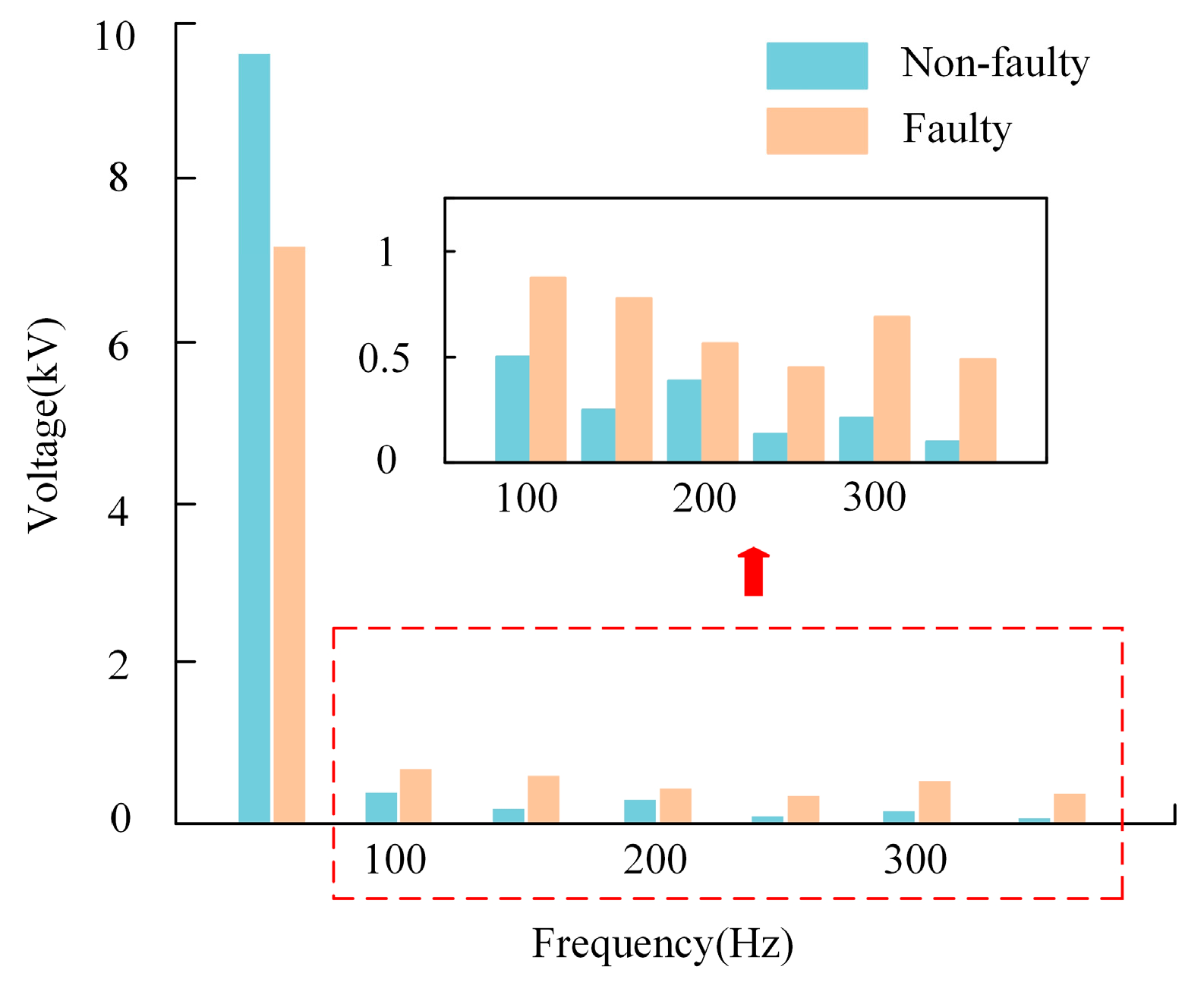
Figure 7 illustrates the voltage and frequency components at measurement point 2 during both normal operation and when a fault occurs on MG line L2. It is evident from the figure that a short-circuit fault in the MG line leads to a notable discrepancy in harmonic voltage components compared to the system’s behavior under normal conditions. This paper opts to utilize the fault voltage and voltage fundamental at the measurement point as characteristic indices to ascertain fault occurrences. Recognizing that voltage frequency is inversely proportional to amplitude, this paper selects low-frequency components at the measurement point as characteristic variables. Specifically, the voltage fundamental and the sixth harmonic components are chosen to determine fault occurrences. During a single cycle of fault occurrence, the three-phase voltage data from each test point are collected, and a Fourier analysis is applied to calculate the voltage amplitude of the fundamental frequency and the sixth harmonic of phase A under fault conditions. The outcomes of these calculations serve as the basis for determining fault occurrences. This method enhances fault detection accuracy by focusing on key voltage characteristics indicative of fault conditions.
- (2)
Fault-type discrimination.
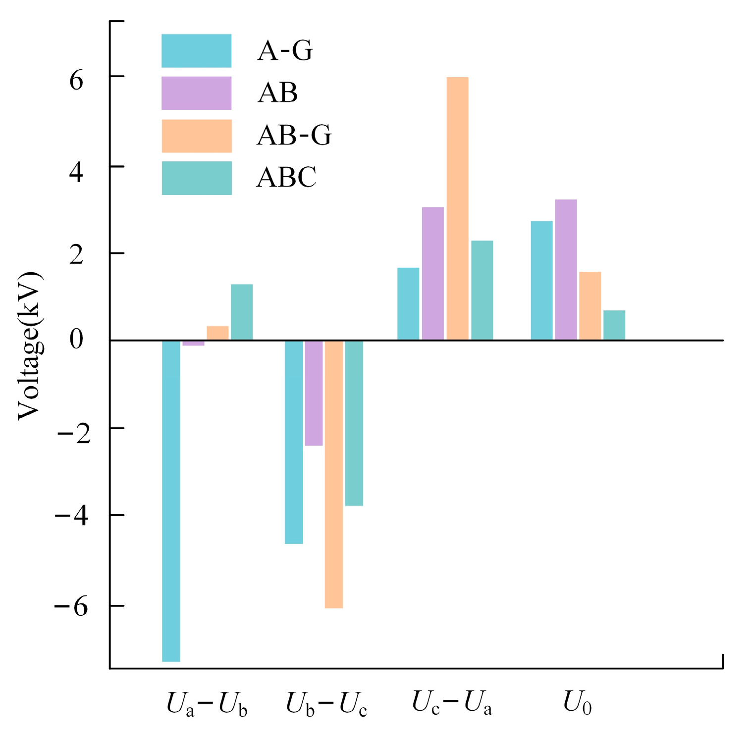
In
Figure 8, when an A-phase single-phase ground fault (A-G), AB phase-to-phase short circuit (AB), AB two-phase ground short circuit (AB-G), and three-phase short circuit (ABC) occur on line L2, there are significant differences observed in the voltage between phases and the zero-sequence voltage at measurement point 2. The Fourier analysis can be utilized to determine the three-phase fundamental voltage amplitude and zero-sequence fundamental voltage amplitude at the measurement points under various operating conditions of the MG. Subsequently, the symmetrical component method can be applied to calculate the difference between the fundamental frequency phase voltages (
Ua—
Ub,
Ub—
Uc,
Uc—
Ua) at each measurement point. This difference, combined with the zero-sequence fundamental voltage, forms the fault-type characteristic quantity at each measurement point. Leveraging this information, the combined model can effectively identify the fault types occurring on MG lines.
- (3)
Fault-location discrimination.
Using the AB-phase short-circuit fault in line L4 as an example, the line fault scenario is simulated. Within a single cycle of the fault, the A-phase voltage data from measurement points 1–4 are extracted. Fourier decomposition is then performed on the A-phase fundamental and harmonic voltage amplitudes to calculate the data under different operating conditions. The obtained data results are compiled into the basic sample set required for training the model for fault-localization identification.
Figure 9 illustrates significant variations in phase voltages at each measurement point across different frequency components. Therefore, by analyzing the low-frequency components of the fault phase voltages at the measurement points and integrating this information with knowledge of the operating state and fault types, the specific lines where MG operating faults occur can be effectively identified.
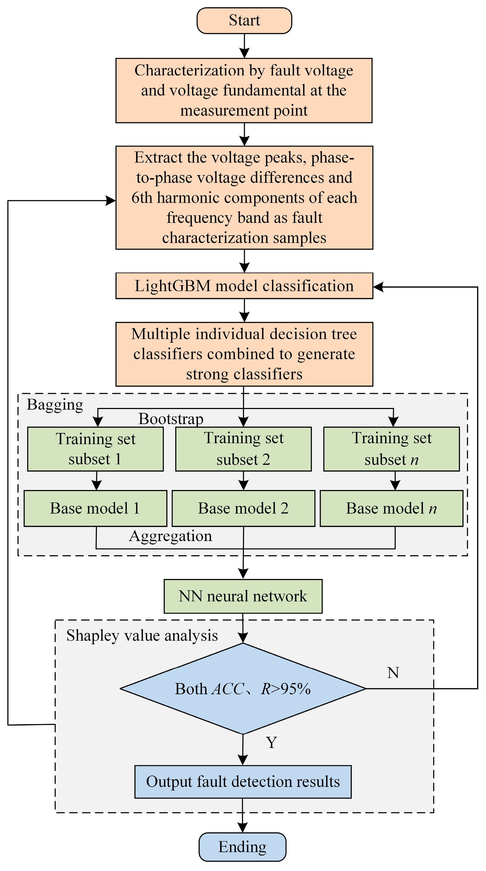
A comprehensive analysis of the three fault detection discrimination methods reveals differences in characteristic quantities across different measurement points. However, the performance of each difference varies. Therefore, it is essential to introduce the Shapley value method for an in-depth study of the contribution of each characteristic quantity in the model’s analytical process. This facilitates the visualization of fault characteristic quantities, allowing the model to prioritize collecting fault feature quantities with higher contribution values. Subsequently, this enables the fault detection function to distinguish between different lines. The fault detection process of the MG based on the LightGBM-NN combined model proposed in this paper is illustrated in
Figure 10.
4.2. Fault Identification Results
In this study, XGBoost, NN, and SVM models sourced from the literature [
9,
11,
12], are employed for comparison with the combined model proposed in this paper. Recognizing the operational realities of MGs in real environments, the signal-to-noise ratio is introduced to investigate the noise immunity of the combined model. This addition allows for a comprehensive assessment of the model’s performance across various conditions, enhancing its applicability and robustness in practical scenarios.
A comparison of line fault-location identification results for different models is presented in
Table 1. The R-value performance of each model is notably strong. However, individual classifiers within the SVM model exhibit simplicity, leading to less accurate fault diagnoses, increased susceptibility to misjudgment, suboptimal model classification, and reduced fitting effectiveness. In contrast, the XGBoost model, equipped with an integrated learning framework, and the NN exhibit minor prediction biases. The LightGBM-NN combined model, utilized in this study, outperforms other models in terms of performance. It not only demonstrates a high recall rate but also exhibits superior generalization ability and exceptional recognition accuracy. These findings provide a solid foundation for the subsequent identification of fault types in MG lines.
To thoroughly investigate the specific impact of introducing the bagging method on the detection performance of the combined model, a comparative study was conducted on the fault line identification accuracy with and without the bagging method based on this MG structure. The comparative results are presented in
Table 2.
Table 2 illustrates a notable improvement in the accuracy of fault identification in both the validation and test sets of the model after the introduction of the bagging method. This finding underscores the effectiveness of incorporating the bagging method in enhancing the generalization ability of the combined model and mitigating the risk of overfitting.
Based on this, various experiments are conducted to test the recognition of different types of line faults using line L9 and measurement point 8 as observation objects. The results of line fault-type recognition by different models are presented in
Table 3. The findings from
Table 3 reaffirm that the LightGBM-NN combined model maintains robust generalization ability compared to other models. Moreover, its classification results for fault-type recognition are the most accurate among all models tested.
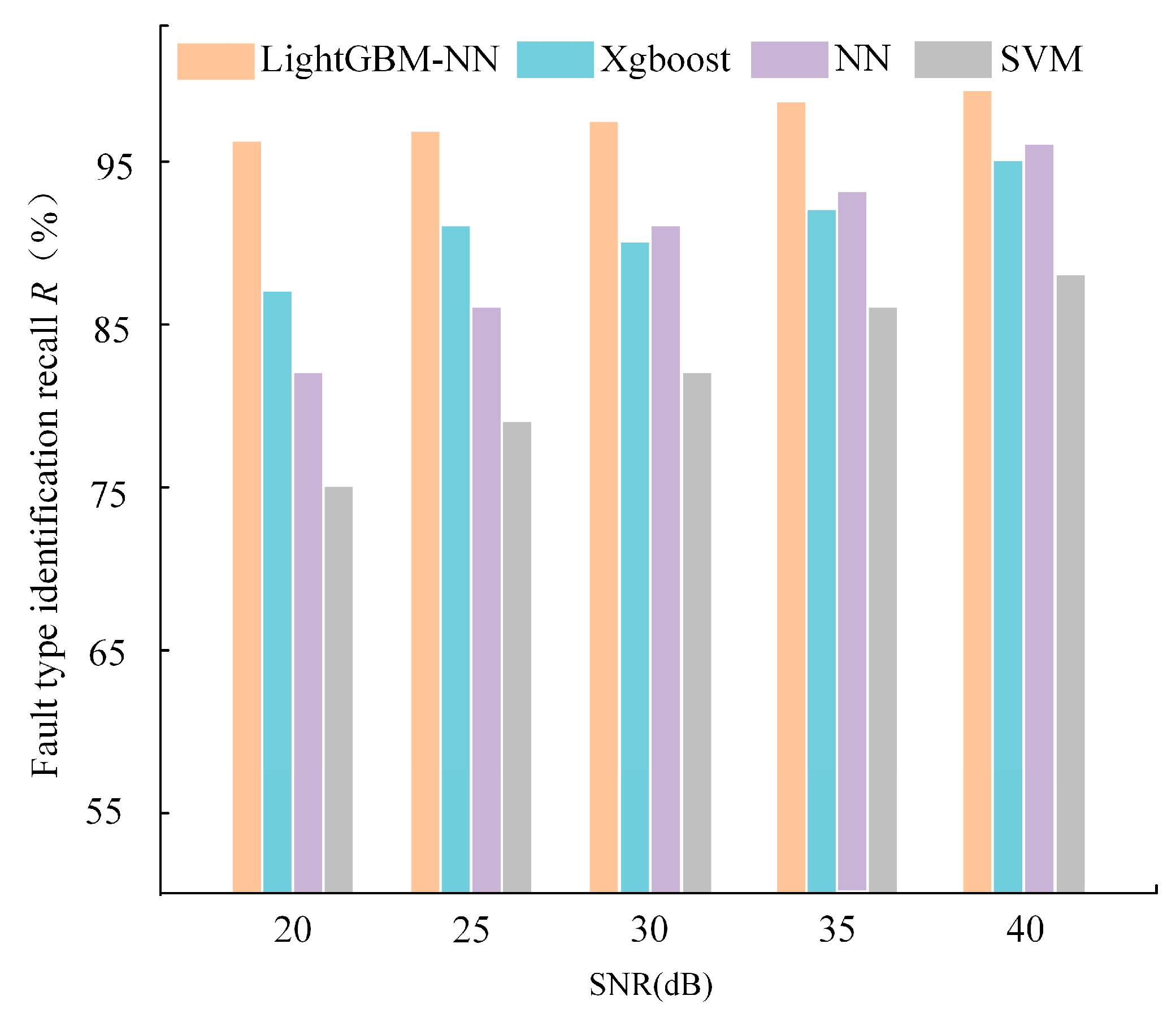
In this paper, to assess the practical applicability of the model, Gaussian white noise, commonly used for analyzing additive noise in communication channels, is introduced. Specifically, signal-to-noise ratios (SNRs) ranging from 20 to 40 dB are applied to observe the noise robustness of the combined model when an A-G fault occurs on line L9, as depicted in
Figure 11.
Across the range of SNRs (20–40 dB), the LightGBM-NN combined model consistently achieves a recall rate of over 95% and maintains high accuracy levels at all SNR levels. Notably, it exhibits the smoothest trend of accuracy improvement with increasing SNRs, showcasing the best performance and robustness to noise. In comparison, XGBoost performs lower than LightGBM-NN at low SNRs but shows a faster performance improvement as SNR increases, indicating its effectiveness on less noisy datasets. The performance of NN improves more smoothly than LightGBM-NN and XGBoost, suggesting its lower sensitivity to changes in SNR.
Conversely, SVM’s performance remains relatively low across all SNRs, particularly at low SNR levels, indicating its heightened sensitivity to noise. In summary, the LightGBM-NN combined model stands out with superior performance, robust noise tolerance, and stable model behavior across varying SNR conditions.
In order to analyze the influence of feature quantities on the localization of a specific fault, the Shapley value method is introduced to rank the features based on their importance.
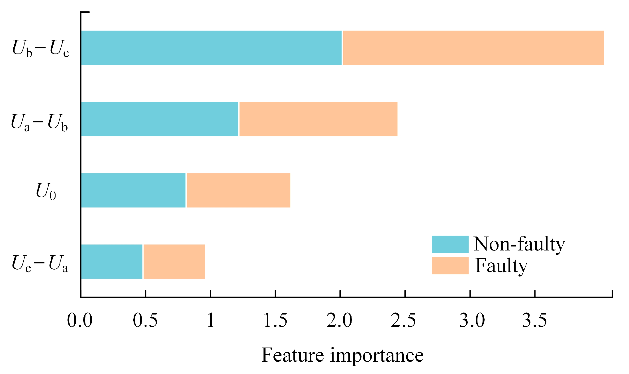
Figure 12 and
Figure 13 depict the feature importance and fault characterization summary diagrams for measurement point 2 when an AB fault occurs on line L2.
Figure 12 illustrates the analysis of the importance of feature quantities in determining the type of fault on line L2.
It reveals that voltage differences between phases and variations in zero sequence voltage at measurement point 2 contribute differently to the model’s determination of fault type for line L2. Among these,
Ub—
Uc exhibits the highest importance when an AB fault occurs on line L2, while
Uc—
Ua demonstrates the lowest importance. Other characteristics of line fault types can be analyzed in a similar manner based on their respective contribution degrees.
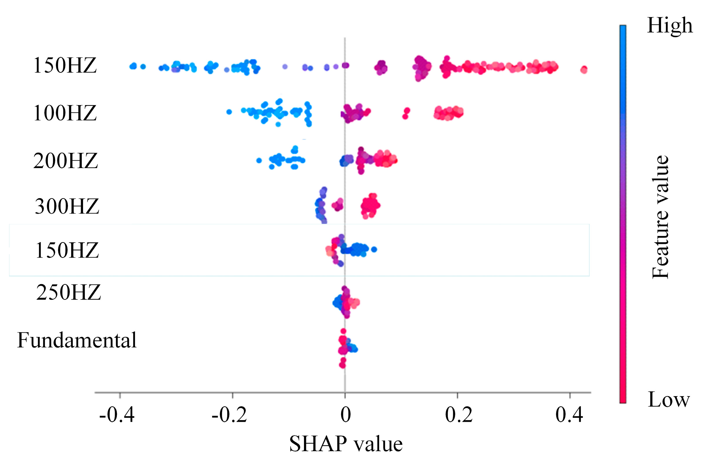
Figure 13 provides a summary of the fault discrimination feature analysis when an AB fault occurs. The SHAP values corresponding to different feature quantities are distributed on both sides of the middle baseline. The position of the dots indicates the positive or negative influence of the feature on the prediction results, while the color shades reflect the magnitude of its influence. Blue represents negative influence, pink represents positive influence, and darker colors represent higher feature values. The size of the scatter indicates the absolute contribution of the eigenvalue to the model prediction. From
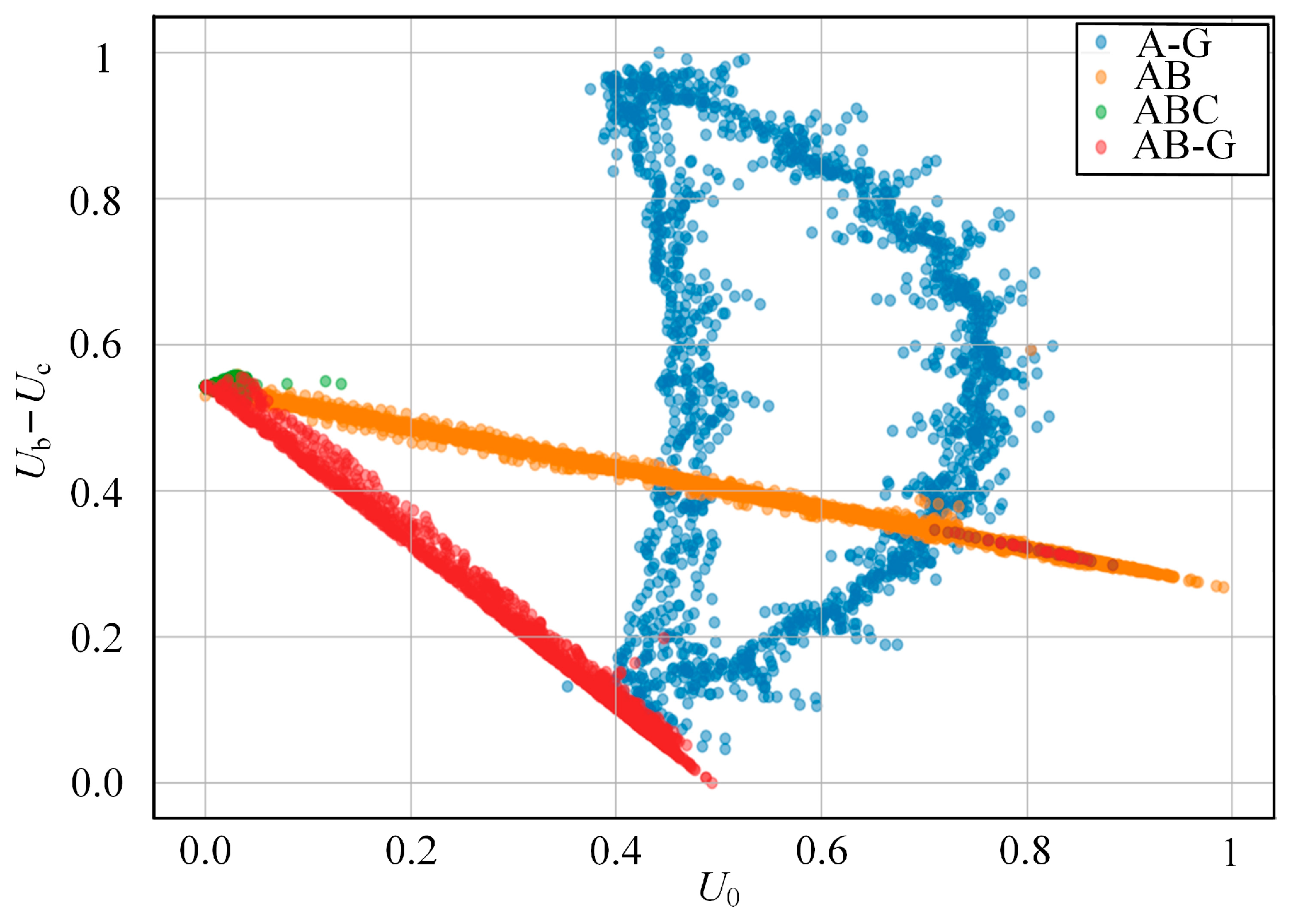
Figure 13, it is evident that the second harmonic (150 Hz) and fifth harmonic (300 Hz) exert a significant influence on the fault-location model. Furthermore, the analysis of voltage differences between phases and the contribution of zero sequence voltage eigenvalues at measurement point 2 for different fault types occurring on line L2 is continued, as depicted in
Figure 14.
When an ABC fault occurs, the majority of green points are clustered in the left region of the horizontal axis, indicating a higher degree of contribution from Ub—Uc compared to U0. This suggests that Ub—Uc plays a more significant role when a three-phase short-circuit fault occurs. However, for AB and AB-G faults, the distribution of points is more evenly spread compared to A-G and ABC faults, indicating that the feature contributions of Ub—Uc and U0 are not as prominent during AB and AB-G faults on line L2 as they are during A-G and ABC faults. Therefore, the Shapley value method offers a visual interpretation of the training data for the model. By identifying a few feature quantities with larger contribution values, the data collection process of the model can be simplified, consequently enhancing its fault-type detection performance.
5. Conclusions
To address the challenge of line fault detection accuracy in MGs with multiple distributed power sources and to mitigate the redundancy in operational data found in existing literature models, this paper proposes a combined LightGBM-NN-based MG line fault detection model incorporating the bagging method and Shapley value analysis. The model’s input dataset includes the characteristic relationship between the peak voltage at each measurement point, phase-to-phase voltage difference, sixth harmonic component, and fault state. Simulation experiments demonstrate that the proposed method enables the visualization of the contribution values of different characteristic quantities in the fault detection process, streamlines the collection of fault characteristic quantities from different lines in multi-terminal active distribution networks, aids in attributing fault diagnostic results, reduces the required data volume for model operation, enhances diagnostic result credibility, and provides effective detection information for fault detection regions in multi-terminal active distribution networks. Additionally, the introduction of the bagging method mitigates issues such as overfitting, enhancing the generalization ability of the combined model. This makes the interpretation of Shapley values more stable and reliable. Experimental comparative studies show that the accuracy and recall of the proposed MG fault detection model exceeds 95% compared to Xgboost, NN, and SVM algorithms. Moreover, even in the presence of Gaussian white noise, the recall rate of fault-type identification remains optimal, demonstrating superior noise robustness and detection accuracy. This method offers valuable insights for future research in MG line fault detection. There are still some shortcomings in this research, and more factors need to be considered for improvement when considering the problem of radial network structure fault detection, so future work will start with the following aspects: (1) The line operation under the networked power system structure is included in the key research direction of combined model fault detection, and the accuracy and stability of model fault detection under the multi-path propagation of faulted lines are considered. (2) The networked line structure of the simultaneous failure of multiple lines is added into the model fault detection focus of the research content. Based on this situation, the model features dual fault detection functions for both networked and radial line structures, aligning more closely with the diverse development requirements of today’s power systems.


