The Impact of Energy Efficiency on Economic Growth: Application of the MARCO Model to the Portuguese Economy 1960–2014

Abstract

The benefits of energy efficiency are recognized in multiple socio-economic spheres. Still, the quantitative impact on macroeconomic performance is not fully understood, as modeling tools are not thermodynamically consistent—failing to explicitly include the useful stage of energy flows and/or thermodynamic efficiencies in primary–final–useful energy transformations. Misspecification in the link between energy use and the economy underplays the role of energy use and efficiency in economic growth. In this work, we develop and implement the Macroeconometric Resource Consumption model for Portugal (MARCO-PT), 1960–2014. Based on the post-Keynesian framework developed for the United Kingdom (MARCO-UK), our model explicitly includes thermodynamic energy efficiency, extending the analysis to the useful stage of energy flows. The model’s stochastic equations are econometrically estimated. The historical influence of key variables—namely thermodynamic energy efficiency—on economic output is assessed through counterfactual simulations and computation of year-by-year output elasticities. The MARCO-PT model adequately describes the historical behavior of endogenous variables. Although its influence has decreased over time, thermodynamic efficiency has consistently been the major contributor to economic growth between 1960–2014, with an average output elasticity of 0.46. Total useful exergy is also a major contributing factor, with an average output elasticity of 0.29. Both have a higher influence than capital, labor, or other energy variables (final energy, prices). An adequate integration of thermodynamic efficiency is thus crucial for macroeconomic models.

1. Introduction

Increasing attention has been given to energy efficiency as a key resource for economic and social development. The multiple benefits approach of the International Energy Agency (IEA) [1] illustrates the vast potential for energy efficiency—a “first fuel”—in areas of macroeconomics, productivity, health, pollution, and energy security, among others.

The area of macroeconomic benefits from energy efficiency is especially important for policymakers and the general public, dealing mostly with the potential role of energy efficiency as a driver (and/or constraint) of economic growth. As a mainstream branch of economic analysis, the macroeconomic assessment has built up a large body of knowledge over many years. Still, the ways by which energy use and energy efficiency influence macroeconomic performance are not yet fully understood. To harvest the potential benefits of energy efficiency—and translate them into policy action—these must be acknowledged not just qualitatively but quantitatively. Comparisons across studies are conflicted by, among other factors, the methods used and the definition adopted for improvements in energy efficiency.

Standard neoclassical growth theory overlooks the role of energy use and energy efficiency, instead attempting to explain observed economics through either capital accumulation or human labor growth but ending up having to attribute a considerable share of historical growth in industrialized countries to a residual term—total factor productivity. Often, total factor productivity is assumed to be exogenous or proxied by indicators that are hard to quantify, a feature that has been carried over to models that forecast economic growth and its implications for climate change (Section 2.1).

Unlike the standard neoclassical approach, in the field of ecological economics, we can find both the recognition of the importance of energy as a driver of economic growth and the argument that its importance is tied to its quality, in a thermodynamic sense, and the stage at which it delivers economic value. The growing research field of exergy economics has uncovered a strong relationship between economic growth and useful exergy consumed. The latter corresponds to energy measured after all conversion processes, at the point where it delivers energy services, and with the exergy metric, considering its potential to perform physical work (exergy content, indicative of energy quality). Previous work that adopts this energy metric has successfully linked it with changes in total factor productivity and economic growth (Section 2.2).

Despite its importance, the insights obtained particularly from the subfield of exergy economics have not found their way into the principal tools of macroeconomic modeling, i.e., computable general equilibrium and macroeconometric models. These two approaches are fairly distinct in their assumptions, flexibility, and assessment. While policymakers benefit from complementing their decision processes with both types of models, as long as they are limited to the final stage of energy flows and fail to acknowledge energy quality, none of them can be considered thermodynamically consistent. Hence, they are ill-equipped to adequately weigh the macroeconomic impacts of changes to energy efficiency (Section 2.3).

To address this shortcoming in macro energy–economy models, the Macroeconometric Resource Consumption (MARCO) model has been developed and originally implemented for the UK economy. This post-Keynesian macroeconometric model explicitly incorporates thermodynamic energy efficiency and extends energy flows to the useful stage. Through counterfactual simulations, the MARCO-UK model concluded that the useful exergy consumed and thermodynamic energy efficiency have had the biggest cumulative impact on historical economic growth, compared both to traditional factors of production and more conventional energy variables (Section 2.4).

We believe it is a logical step to adapt and implement the MARCO framework in other developed economies to compare results. Hence, the present work does this for Portugal 1960–2014. Section 2 details the background and motivation summarized above. The methods detailed in Section 3 address some conceptual shortcomings of the original MARCO-UK and, therefore, constitute a better blueprint for the future implementation of the model in other economies. The results presented in Section 4 are compared with those of the MARCO-UK and discussed in the context of previous findings concerning the link between useful exergy, efficiency, and economic growth in the Portuguese economy. Section 5 concludes and points out directions for future work.

2. Background and Motivation

2.1. Neoclassical Growth Theory—Ignoring the Role of Efficient Energy Use

Growth accounting is one of the workhorses of mainstream empirical analyses of economic growth [2,3,4,5].

The most basic mainstream neoclassical growth models consider capital accumulation and human labor as the only two factors of production contributing to economic output. These factors are weighed by their respective shares of payments in national accounts—capital paid in operating surplus (rents, profits) and labor paid in compensation of employees (wages, salaries)—and combined and corresponded to a level of output via an aggregate production function (APF), generally of the Cobb–Douglas type—Equation (1),

$$Y=A·K^{{\alpha }_K}·L^{{\alpha }_K}$$

(1)

where $Y$ is gross domestic product (GDP), $K$ is capital, $L$ is labor, ${\alpha }_K$ and ${\alpha }_L$ are the cost shares, and $A$ is an exogenous multiplier term, often called the total factor productivity (TFP).

While neoclassical growth theory expects the combined contribution from capital and labor to be sufficient in accounting for historical economic growth, empirical work has repeatedly shown that this is not the case for developed economies. In his landmark growth accounting paper, Robert Solow concluded that the exogenous TFP term $A$ in Equation (1)—a “Solow residual”—accounts for over 85% of US growth (1909–1949). Since Solow’s original results, residual TFP has been pointed out as the major driver of growth in industrialized economies [6].

In dealing with the problematic concept of TFP, a strand of research has proposed to accept it and look for the underlying factors that explain TFP changes—whether wanted (technical and/or organizational innovation [7]) or unwanted (measurement errors, omitted variables, aggregation bias [8,9,10,11,12,13]). However, while the combined efforts have led to captivating avenues of research, a better understanding of the drivers of growth, and additions to countries’ statistical repositories [2,3,4,5,14,15], a considerable portion of TFP cannot be “explained away” by either refined measurements of capital and labor or considering broader investment concepts or technological spillovers [16].

Other strands of research opt to look beyond the concepts of the neoclassical production function, TFP, and their simplifying assumptions and limitations. The aggregate production function is open to critique due to “aggregation issues”: the condition under which heterogeneous outputs and inputs can be summed across micro-production functions to give an APF are so stringent that it is hard to believe such an aggregate function exists [17,18]. The arguments concerning the aggregation problem state that the APF is merely capturing an underlying accounting identity, which explains the good statistical fits commonly obtained. The implications for empirical analysis include—but are not limited to—the fact that the elasticity of substitution estimates does not reflect technological parameters [17,19]. Also, the famous Cambridge “capital controversy”, sparked by the work of Piero Sraffa and Joan Robinson [20,21], pointed out that the aggregate measurement of capital inputs involves adding up incomparable heterogeneous assets. The aforementioned studies constitute key moments in post-Keynesian macroeconomic theory [22]. Post-Keynesian economics rejects the methodological individualism that underlies much of mainstream economics. It also rejects the need for optimizing microfoundations and the concept of long-run supply-side equilibrium while maintaining that aggregate demand matters both in the short and the long run. Supply operates as a potential constraint on economic expansion, driving growth only when they effectively restrict demand (e.g., in a scenario of full employment, the increase of labor productivity becomes imperative for the elevation of overall output).

Regardless of how economic growth is justified, it is important for policymakers to understand what drives it and how it can be modeled. It is not uncommon for widely used economic growth scenarios to be built upon neoclassical aggregate production functions, relying on projections for TFP that are either exogenous to the model or based on several—often abstract—indicators (innovation, education, institutions, etc.) [23]. Most of the Integrated Assessment Models (IAMs) that inform mitigation scenarios of the Intergovernmental Panel on Climate Change (IPCC) resort to neoclassical production functions and tend to treat TFP—and therefore most of economic growth—as exogenous [24], risking low confidence in the quantitative predictions of such models [25].

2.2. Ecological Economics—Energy’s Potential to Perform Work as a Driver of Growth

While providing a poor explanation for the drivers of economic growth, the basic neoclassical approach also—notably—omits energy from its framework. The often-cited argument [26] is that energy, allocated a considerably smaller share of payments in national accounts, has a negligible productive power when compared to capital or labor. Intuitively, it is hard to believe that production can be modeled without an essential role for energy. In fact, misspecification in the interactions between energy and economic production might account for the relevance attributed to residual TFP as the major driver of growth. That is, at least, the predominant view in the field of ecological economics.

Within this field, there is a vast literature dedicated to introducing energy, in some form, into the aggregate production function framework alongside capital and labor. Initial attempts still assumed perfect (or almost) substitution among factors [27,28,29,30,31], but subsequent econometric analyses find evidence for complementarity (or weak substitutability) [32,33] and introduce more realistic constraints on energy–capital substitution [34,35,36,37]. While concluding that energy scarcity will hamper future growth, most of these models still assume indefinite TFP growth can assure economic development.

Other strands of work have focused directly on the link between energy efficiency changes and the rate of economic growth. While uncovering evidence that the two are positively correlated, the definition of energy efficiency—i.e., what is meant by it and what is included—varies between different studies. Generally, this definition is based on the first law of thermodynamics—the conservation of energy principle—and on transformations from the primary to final stages of energy flows (e.g., electricity generation from coal). However, first law efficiencies fail to acknowledge energy degradation due to irreversibilities and changes in energy quality [38]. Stopping at the final stage of energy flows also fails to account for energy delivered to economically productive end-uses and services.

The matter of energy quality can be assessed by redefining energy efficiency to consider the second law of thermodynamics. While energy is conserved, the exergy content of energy—its potential to perform physical work, i.e., to be productive, decreases as energy is transformed [39]. Second law (exergy) efficiencies account for energy quality in a comparable way. The benefits of shifting the focus from an energy to an exergy perspective are acknowledged by several institutions [40]. The definition of energy (or exergy) efficiency must also be extended to encompass the useful stage of energy/exergy flows responsible for delivering economic value (e.g., electricity converted to light in a lightbulb) [41]. The final-to-useful transition is, in fact, where most thermodynamic losses occur (Figure 1).

The second law definition for thermodynamic energy efficiency has sparked new insights regarding the contribution of energy to economic growth (motivated by the increasing data availability on final and useful exergy consumption from societal accounting studies [43,44,45,46]). Historically, economic growth has depended on increases in the supply of useful exergy, achieved through a combination of increasing primary/final energy supply, shifting towards higher-quality carriers (e.g., oil to electricity), and improving the efficiencies at all stages of the energy conversion chain [42,46,47,48,49,50,51,52,53]. These insights have led to models for economic output that eliminate the need for exogenously driven TFP growth, representing instead the dynamics of technological progress in terms of increasing the efficiency of exergy conversion from the primary to the useful stage [42,46].

While relevant, these models do not fully capture the quantifiable macroeconomic impacts of changes in energy efficiency. Modeling the complex interactions between energy, production, prices, employment, and/or the environment requires advanced tools, i.e., macroeconomic energy–economy models.

2.3. Energy–Economy Models at the Macro Level and Their Limitations

The primary advanced methodologies for simulating the macroeconomic effects of alterations in energy efficiency are computable general equilibrium (CGE) models and macroeconometric models. These analytical frameworks find application across governments, international organizations, enterprises, and academia in evaluating economic and energy-related policies [54,55,56,57]. While both methods share notable resemblances, with their core reliance on social accounting matrices, they also exhibit significant disparities, particularly concerning the treatment of human behavior.

CGE models are based on a standard Arrow-Debreu [58] general equilibrium framework, drawing on neoclassical macroeconomic theory. These models can be comparative static or dynamic [59]. The former focuses on modeling the reactions of the economy at only one point in time, while the latter focuses on modeling dynamic adjustment paths. Perfect knowledge of agents is assumed, which allows modeling optimizing behavior, something CGE models almost always do. Frictionless markets allow price adjustments to balance supply and demand [60] (newer generations allow for market imperfections [61]). These models prove useful when studying economies of countries for which time series data are scarce and can be replaced by strong, reasonable assumptions embedded in the model.

The approach generally adopted by macroeconometric models draws on Keynes’ analysis that the best estimates of future behavior are the trends that one can currently observe [62]. These models allow for the possibility of fundamental uncertainty; hence, modeling optimizing behavior is not possible. The economy is conceptualized as a non-equilibrium system in the sense that markets are often inefficient, and prices do not automatically adjust to market-clearing levels [63,64]. Without optimization, macroeconometric models resort to alternate assumptions to populate model parameters. Historical trends are assumed to be the best estimates of future behavior, and econometrics provides the best tools to derive quantitatively the behavioral relationships. One advantage of these models compared with the CGE approach is that they enable counterfactual simulations to be run over the model’s time frame, isolating the effects caused by changes to any variable on the whole economy. Such simulations have the flexibility to cause disequilibrium, propagation of disturbances, and policy effects over the system [65].

Policy insights are highly dependent on the economic assumptions in each type of model. CGE models provide an assessment of how the optimal use of available resources might change, given a set of policy constraints. Macroeconometric models also provide an assessment of how resource efficiency might change, but in addition, they show the impacts of using more or less available resources. While introducing a regulatory policy in a CGE model constitutes an additional constraint—and output can only decrease—in a macroeconometric model, the same policy can increase the level of output if it is able to draw on previously idle resources. Ultimately, it is unlikely that any single model can capture all relevant economy-wide effects of energy efficiency. Policymaking benefits from exploring the complementarity of both CGE and macroeconometric models.

Regardless of their differences and similarities, both types of economy-wide models currently employed [66,67] cannot be considered thermodynamically consistent. Despite including capital, labor, and (primary or final) energy use as key inputs to production [68,69], they do not explicitly include thermodynamic efficiency and the useful stage of energy/exergy use or energy services. This is a very significant omission, especially considering the recent findings on the links between energy/exergy efficiency and economic growth, as summarized in Section 2.2.

2.4. The Thermodynamically Consistent MARCO Model

The MARCO (Macroeconometric Resource Consumption) model represents a pioneering step in energy–economy-wide modeling, incorporating thermodynamic efficiency and energy services as explicit components [50]. Distinguishing itself from previous macroeconometric models [70,71], the MARCO introduces the concept of the useful stage of energy/exergy consumption (following the “energy carriers for energy use” thermoeconomics-based exergy analysis boundaries [39,72], as opposed to the extended exergy analysis boundary [52,53]), serving as a proxy for energy services.

Being a post-Keynesian macroeconometric model, its development is rooted in empirical data, highlighting the significance of aggregate demand in propelling economic expansion while supply adapts to fulfill this demand. Borrowing from the principles of ecological economics, the model posits energy and capital as predominantly complementary inputs. Rather than depending on exogenous TFP, the MARCO model internalizes technical advancements, attributing all economic growth to factors within the model. Counterfactual (ex-post) simulations enable explicit isolation and measurement of the impact of improvements in thermodynamic efficiency and useful exergy on economic growth.

Applied to the United Kingdom’s economy over the past five decades, the MARCO-UK model reveals that thermodynamic exergy efficiency—in conjunction with capital investment—consistently exerts a significant influence on GDP growth [50]. When thermodynamic efficiency was restricted to 1971 levels, there was a notable 25% reduction in GDP by 2013, corroborating earlier findings in ecological economics [42,46,48]. Moreover, the MARCO-UK model underscores that useful exergy has a higher impact on economic growth than either final energy or energy prices, aligning with assertions in ecological economics regarding the close connection between useful exergy and economic growth [42,49,73,74,75].

The United Kingdom has demonstrated comparable economic growth and patterns of structural transformation, along with advancements in thermodynamic efficiency, akin to other industrialized nations. Hence, it is legitimate to ask whether the findings of the original application of the MARCO-UK model are replicable in other developed economies. To address this, the present work focuses on the development and application of the MARCO modeling framework to the Portuguese economy (PT) over the past 50 years.

Portugal is a good candidate for this type of analysis: in the last 50 years, there have been both periods of considerable improvements and stagnation in the thermodynamic final-to-useful energy/exergy efficiency of the country [44,76]. Furthermore, previous analyses carried out with Portuguese energy/exergy and economic data have uncovered robust evidence of a close relationship linking thermodynamic efficiency with total factor productivity [42] and overall useful exergy consumption with economic growth [49]. These observations make Portugal an interesting choice for a proof-of-concept expansion of the MARCO model beyond the UK economy. The methodology presented in the next section can be implemented for other economies in the future and the obtained results compared with those presented in this work and in the original MARCO-UK paper.

3. Materials and Methods

The MARCO-PT, like its UK counterpart, is a model with post-Keynesian characteristics in the sense that aggregate demand drives economic growth, and supply adjusts to meet demand.

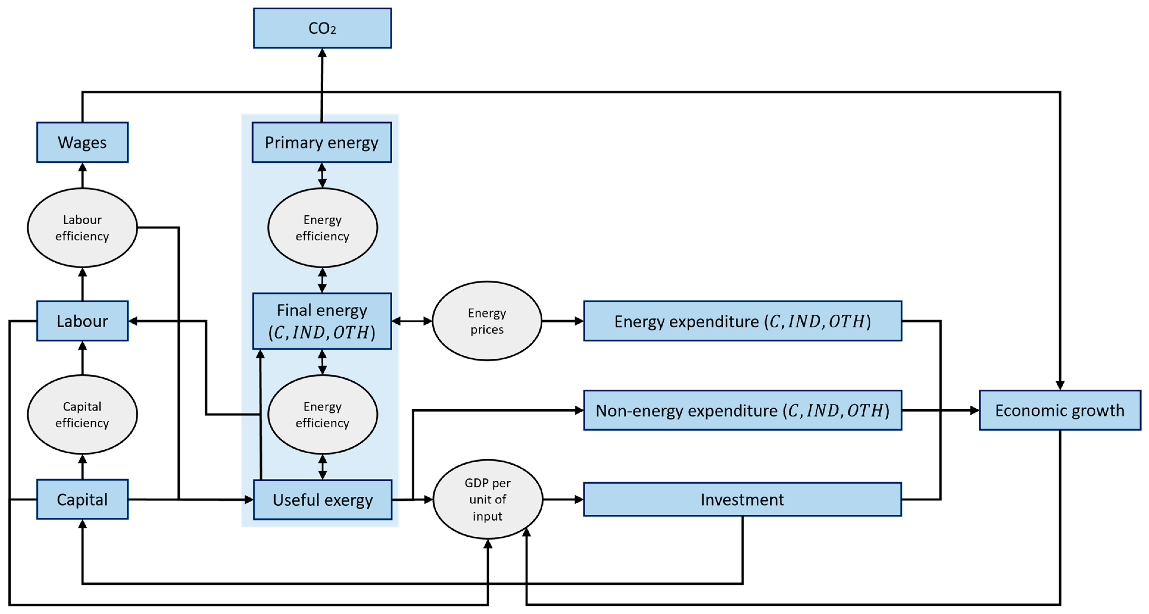
The MARCO-PT framework integrates principles from ecological economics, specifically recognizing energy’s indispensability within the economic system and the predominantly complementary relationship between energy and capital inputs (on the one hand, additional energy is required to operate an extra machine and, on the other hand, investment in capital is also required to activate energy efficiency gains). Energy flows are traced beyond the primary and final stages, extending to the useful stage just prior to conversion into energy services. These useful energy flows are quantified in terms of exergy, accounting for both their quantity and quality in the economy. The transition between energy stages is governed by two types of thermodynamic efficiencies: primary-to-final and final-to-useful. An enhancement in final-to-useful efficiency allows the same quantity of final energy to yield a greater amount of useful energy.

Thus, key energy variables within the MARCO-PT model encompass energy consumption across primary, final, and useful stages, along with thermodynamic efficiencies at both the primary-to-final and final-to-useful transitions, quantified in exergy units. At the final energy stage, three sectors contribute to energy consumption: households (C), industry (IND), and others (OTH, such as agriculture, government, and services). Figure 2 depicts a simplified schematic representation of the MARCO-PT model’s structure.

3.1. Model Equations

Two different types of equations constitute the model: (a) definitional or identities; (b) econometric or stochastic (or behavioral). Definitional equations are based on the identities of the system of national accounts. For example, by the expenditure approach, GDP ($Y$) is the sum of private consumption ($C\_T$), government consumption ($G$), investment ($I$), and the trade balance ($X-M$):

$$Y_t=C\_T_t+G_t+I_t+X_t-M_t$$

(2)

Equation (2) is an identity that holds true for all time. So are the following two identities, based respectively on the income and production approach to measure GDP:

$$Y_t=Y{F}_t+W_t+NE{T}_{{TAX}_t}$$

(3)

$$Y_t=GV{A}_t+NE{T}_{{TAX}_t}$$

(4)

where $YF$ is the gross operating surplus, $W$ is compensation of employees, $GVA$ is gross value added (at basic prices), and $NET\_TAX$ is net taxes on production.

The stochastic equations within the MARCO-PT model are grounded in empirical data, with parameters estimated through econometric methods. These equations establish connections among several crucial variables in the model. For instance, labor supply ($L$) is determined by GDP ($Y$) and other factors of production, including capital services ($K\_SERV$) and useful exergy ($UEX\_TOT$)—as expressed in Equation (5). Similarly, investment expenditure ($I$) is influenced by factors such as firm profits ($YF$), capital productivity ($Y/K\_NET$), labor productivity ($Y/L$), and the efficiency of useful exergy consumption ($Y/UEX\_TOT$)—as depicted in Equation (6).

$$L_t=f\left(Y_t,K\_SER{V}_t,UEX\_TO{T}_t\right)$$

(5)

$$I_t=f\left(Y{F}_t,Y_t/K\_NE{T}_t,Y_t/L_t,Y_t/UEX\_TO{T}_t\right)$$

(6)

The MARCO-PT model includes 29 identities and 25 stochastic equations. All equations are listed in the Supplementary Materials (Section S1). Data corresponding to all variables included in the model is referenced in Supplementary Materials (Section S2).

The variables and parameters of stochastic equations, such as Equations (5) and (6), are tested by employing suitable econometric techniques. Coefficients are derived from ordinary least squares (OLS) regression with log-transformed variables [77]. Estimated coefficients are scrutinized for statistical significance and conformity with theoretical predictions. The stochastic equations are also assessed for their goodness-of-fit and covariance in forecasting the dependent variable based on variations in the independent variables. Residuals are examined for normality, homoskedasticity, and serial correlation. For each stochastic equation, the existence of a common long-term equilibrium relationship between variables is tested using appropriate stationarity and cointegration techniques [78]. If no evidence of cointegration is detected, the dependent variable is modeled with short-run dynamics only (lagged terms) in a vector autoregressive (VAR) model. If cointegration is detected, the dependent variable is modeled with both short-run and long-run dynamics—the latter an error-correction term—in a vector error-correction model (VECM).

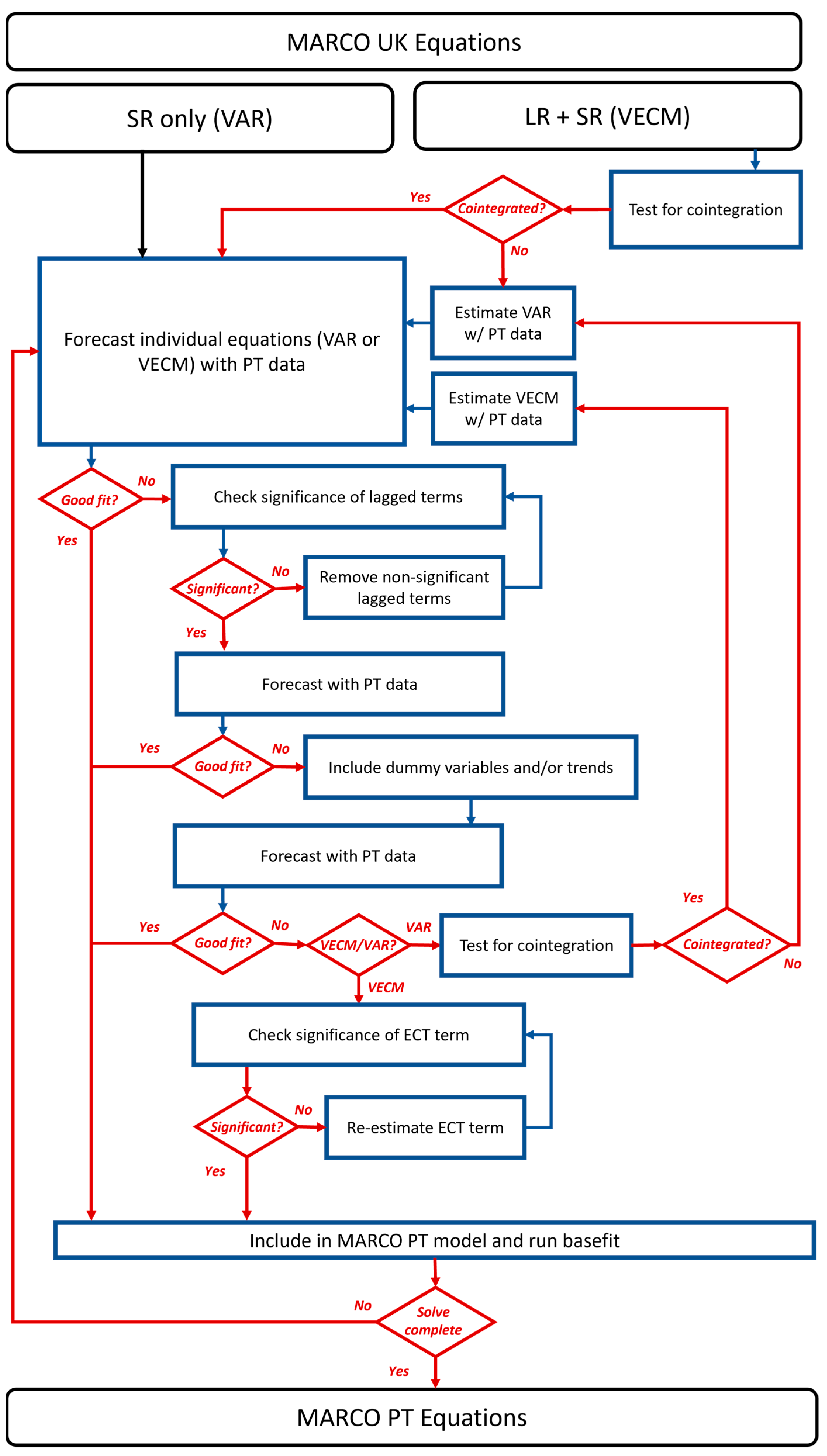
The estimation of stochastic equations is the core of the development and implementation of the MARCO-PT model. Truly, the stochastic equations are the model. In this paper, this estimation is conducted by taking as a starting point the stochastic equations previously determined for the MARCO-UK model [50]. The reasoning for this is that we wish to evaluate whether (or how well) the framework of the MARCO-UK model adapts to the characteristics of the Portuguese economy. The iterative process by which the stochastic equations for Portugal are estimated and incorporated into the MARCO-PT model is summarized in the flowchart of Figure 3 and detailed below.

The VECM stochastic equations in the MARCO-UK model—with both long-run and short-run terms (LR+SR)—are econometrically tested with data for Portugal. This means testing each individual variable time series for stationarity through appropriate unit root tests—Augmented Dickey–Fuller [79] and Phillips–Perron [80]. It also means testing for cointegration among the variables using the trace and max-eigenvalue statistics of the Johansen procedure [78]. The Johansen procedure can test up to $n-1$ cointegrating relationships among variables, where $n$ is the number of variables included in the cointegration space. If variables are integrated in the same order, and cointegration is observed, the VECM formulation is adopted to forecast the dependent variable. On the other hand, if econometric testing fails to detect cointegration for Portuguese data, the VECM is reformulated as a VAR with short-run terms only (SR).

If stochastic equations—VAR or VECM—taken from the MARCO-UK model, when re-estimated for Portugal (what is meant, throughout this paper, as directly adopting an equation from the MARCO-UK model to include in the MARCO-PT model, is, in fact, taking the form of the MARCO-UK equation and re-estimating its parameters with data from Portugal), show a good fit to historical data, statistically significant coefficients, acceptable values for normality, serial correlation, and homoscedasticity test statistics, and high covariance in forecasting the dependent variable, then these stochastic equations are included in the MARCO-PT model to run a basefit solution.

When the stochastic equations taken from the MARCO-UK model fail to accurately fit Portuguese historical data; and/or forecast dependent variables with a high level of covariance; and/or test statistics for normality, homoscedasticity, and serial correlation fall outside acceptable values; and/or coefficients are not significant, then the stochastic equation enters an iterative process of re-evaluation and re-estimation, as illustrated in Figure 3. The statistical significance of estimated coefficients for lagged terms is checked, and non-significant lagged terms are removed. Dummy variables and trends are included to account for breakpoints or other sui generis moments in Portuguese economic history (most notably, the Democratic Revolution of 1974), and their statistical significance is also assessed. If the sign of any given independent variable goes against the theoretical expectation for that variable in the economy (e.g., a rise in energy prices has a positive effect on energy use), the equation is also re-evaluated.

Building the MARCO-PT model framework is, therefore, an iterative process. Re-evaluating a given stochastic equation according to one criterion (e.g., inclusion of dummy variables) might afterward demand re-evaluating the same equation according to a different criterion (e.g., after including a dummy variable, some lagged terms are no longer significant). In this sense, the process is one of trial and error until satisfactory equations are obtained.

Once all individual stochastic equations are estimated for Portugal and deemed statistically robust and adequate to fit/forecast historical data, they are included in the MARCO-PT modeling framework and used in obtaining a basefit solution to the model (Section 4.2). Details on the statistical tests carried out throughout the iterative process illustrated in this section are presented in the Supplementary Materials (Section S3).

3.2. Data

Annual time series data are collected for Portugal, mirroring as much as possible the list of macroeconomic, energy, and environmental variables included in the application of the MARCO model to the UK economy (due to lack of data availability, the MARCO-PT model does not include annual time series data on net wealth/total net worth, money supply – M4) – or consumption-based CO₂ emissions).

The sources of data that feed the MARCO-PT model are listed in the Supplementary Materials (Section S2) for all considered variables. Most national account data on expenditure (consumption, investment, trade) and income (gross operating surplus, compensation of employees, gross value added), as well as capital inputs, are obtained from the macroeconomic database of the European Commission (AMECO) [81]. Data on human labor (engaged individuals, hours worked, population) are obtained from the Penn World Tables (PWT10.0) [3]. Data on primary, final, and useful energy and exergy use, along with the corresponding efficiencies, are obtained from the work of [44,76]. Data on energy prices are obtained from Portuguese-specific databases—that of the Directorate-General for Energy and Geology (DGEG) [82] and the Banco de Portugal long-time series [83]. Additional data are obtained from Eurostat [84] (heating degree days), the World Bank [85] (GDP from the rest of the world), the global carbon atlas [86] (CO₂ territorial emissions per capita), and specific papers [87] (capital services).

The time period covered by all annual time series included in the implementation of the MARCO-PT model is 1960–2014. This range is justified by the best available energy/exergy datasets for Portugal at the time of this analysis [44,76], which have not yet been extended beyond 2014. However, these same datasets have the advantage of covering a significantly long time period going back as far as 1960. Future iterations of the MARCO-PT model will make use of updated energy/exergy datasets for more recent years.

3.3. Basefit Model and Validation

The set of all definitional (i.e., identities) and stochastic equations discussed in the previous section forms the framework of the MARCO-PT model. A complete list of the formulation and estimated coefficients for all equations included in the MARCO-PT model is presented in the Supplementary Materials (Section S4).

Once all equations are determined and the model is finalized, it is dynamically solved using the Gauss–Seidel iterative method [88]. This allows for the determination of annual values for the endogenous variables in the model based on the known values of exogenous variables and on the known initial values of the endogenous variables themselves.

If the Gauss–Seidel method fails to converge or converges towards a solution that does not accurately describe the historical values for one or more of the variables in the model, the corresponding individual stochastic equations are re-evaluated according to the process described in Figure 3. Re-evaluation and re-estimation of the model are repeated until an acceptable basefit solution—one that adequately estimates the historical values for each of the endogenous variables in the model—is obtained from Portuguese data. This basefit solution forms the scenario against which all other scenarios based on counterfactual simulations are compared.

3.4. Counterfactual Simulations and Output Elasticities

As previously mentioned, after a satisfactory basefit solution to the MARCO-UK model has been achieved, Ref. [50] carry out a series of counterfactual simulations aiming, primarily, at understanding the role of thermodynamic final-to-useful exergy efficiency in historical economic growth, when compared with other plausible factors. The ability to perform such isolation provides an advantage over other modeling approaches, e.g., CGE models [89,90].

The counterfactual (ex-post) simulations for the UK in [50] were run for 1971–2014, isolating the cumulative effect on economic output (GDP) caused by keeping a given variable in the model (e.g., thermodynamic efficiency) constant and equal to its value at the beginning of the period.

Here, we acknowledge the advantage provided by the MARCO framework to perform counterfactual simulations but avoid using it in such a way as to bring the model outside the space for which it has been calibrated in its basefit solution. So, instead of constraining selected model variables to their initial values and studying the cumulative effects on GDP for the whole timeframe, we opt to constrain the same selected variables for a single year and evaluate the effect on GDP in the following year. This process is then repeated for every year in the timeframe, and an average output elasticity is computed for every selected variable, by taking the geometric mean of year-by-year elasticities.

Specifically, we take a given variable in the MARCO-PT framework ($Z$), and for a given year ($t-1$ to $t$), assume that the annual growth rate was a fraction ($\gamma$) of the corresponding growth rate of the basefit estimate for this variable. Then, we compare the projected value for the variable at $t$, assuming a growth rate that is $\gamma$ times that of basefit, with the estimate for the variable in the basefit for the same year—Equation (7).

$$\frac{{Z^{\prime }}_t}{Z_t}-1, with {Z^{\prime }}_t=\gamma ·\left[1+\left(\frac{Z_t-Z_{t-1}}{Z_{t-1}}\right)\right]·Z_{t-1}$$

(7)

For each such counterfactual simulation, the MARCO-PT is run, and the projected economic output at $t+1$ (${Y^{\prime }}_{t+1}$) is compared with the corresponding value in the basefit simulation ($Y_{t+1}$)—Equation (8).

$$\frac{{Y^{\prime }}_{t+1}}{Y_{t+1}}-1$$

(8)

An output elasticity for the year $t+1$ is obtained as the quotient of Equation (8) by Equation (7) as in Equation (9):

$${\epsilon }_{t+1}^{Z,Y}=\frac{\left(\frac{{Y^{\prime }}_{t+1}}{Y_{t+1}}-1\right)}{\left(\frac{{Z^{\prime }}_t}{Z_t}-1\right)}$$

(9)

Repeating the same process for every year in the time frame ($n$ being the number of years) and taking a geometric mean of yearly output elasticities obtained from Equation (9), we compute an average output elasticity for each variable $Z$, for the whole period as in Equation (10).

$${\widehat{\epsilon }}^{Z,Y}={\left({{\displaystyle \prod }}_{t=1960}^n{\epsilon }_{t+1}^{Z,Y}\right)}^{\frac{1}{n}}$$

(10)

The output elasticity of Equation (10) tells us, on average, how much of a percentual change in economic output can be attributed to a 1% increase in the selected model variable $Z$. Being computed on a year-to-year basis, our approach evaluates the effect on economic output from selected variables without forcing the model to generate scenarios outside of its calibrated space.

We select for our analysis six variables to test their effect on economic output. These variables are listed below:

• Thermodynamic final-to-useful aggregate exergy efficiency ($EXEFF\_FU$).
• Total final energy use (sum of households $FEN\_C$, industry $FEN\_IND$, and other $FEN\_OTH$).
• Investment expenditure ($I$).
• Labor supply (in number of employees $L$).
• Energy prices (paid by households $P\_EN\_C$, industry $P\_EN\_IND$, and others $P\_EN\_OTH$).
• Total useful exergy ($UEX\_TOT$).

4. Results and Discussion

4.1. Econometric Test Results

Detailed results from econometric tests carried out on the model’s variables and equations can be found in the Supplementary Materials (Section S3).

Stationarity tests suggest that the majority of variables are integrated of order one—I(1), i.e., stationary in first differences but not in levels. The hypothesis that time series are integrated of a higher order than one cannot be rejected for variables measuring capital stock and services ($K\_GRS$, $K\_NET$, $K\_SERV$) and the consumer price index ($CPI$). The reason for this may be that when the alternative is an autoregressive parameter near unity (which must be seen as the empirically relevant case when testing common macroeconomic variables), the power of Dickey–Fuller-type tests is known to be low [91,92]. Throughout the analysis, we assume all variables to be I(1). This is relevant for cointegration testing since the Johansen procedure requires that time series be integrated in the same order.

Cointegration tests suggest that, for each stochastic equation in the model, there is at least one cointegration relationship linking the dependent and independent variables in a long-run equilibrium. The hypothesis of more than one cointegration relationship cannot be rejected for some stochastic equations. But, for the present work, we opt to consider only the alternative hypothesis of, at most, 1 cointegrating relationship. Yet, exploring the detected additional cointegrating relationships for groups of variables in some stochastic equations should be a priority in future iterations of the MARCO model.

4.2. Basefit Solution

Estimated coefficients for each of the stochastic equations in the model are shown in the Supplementary Materials (Section S4).

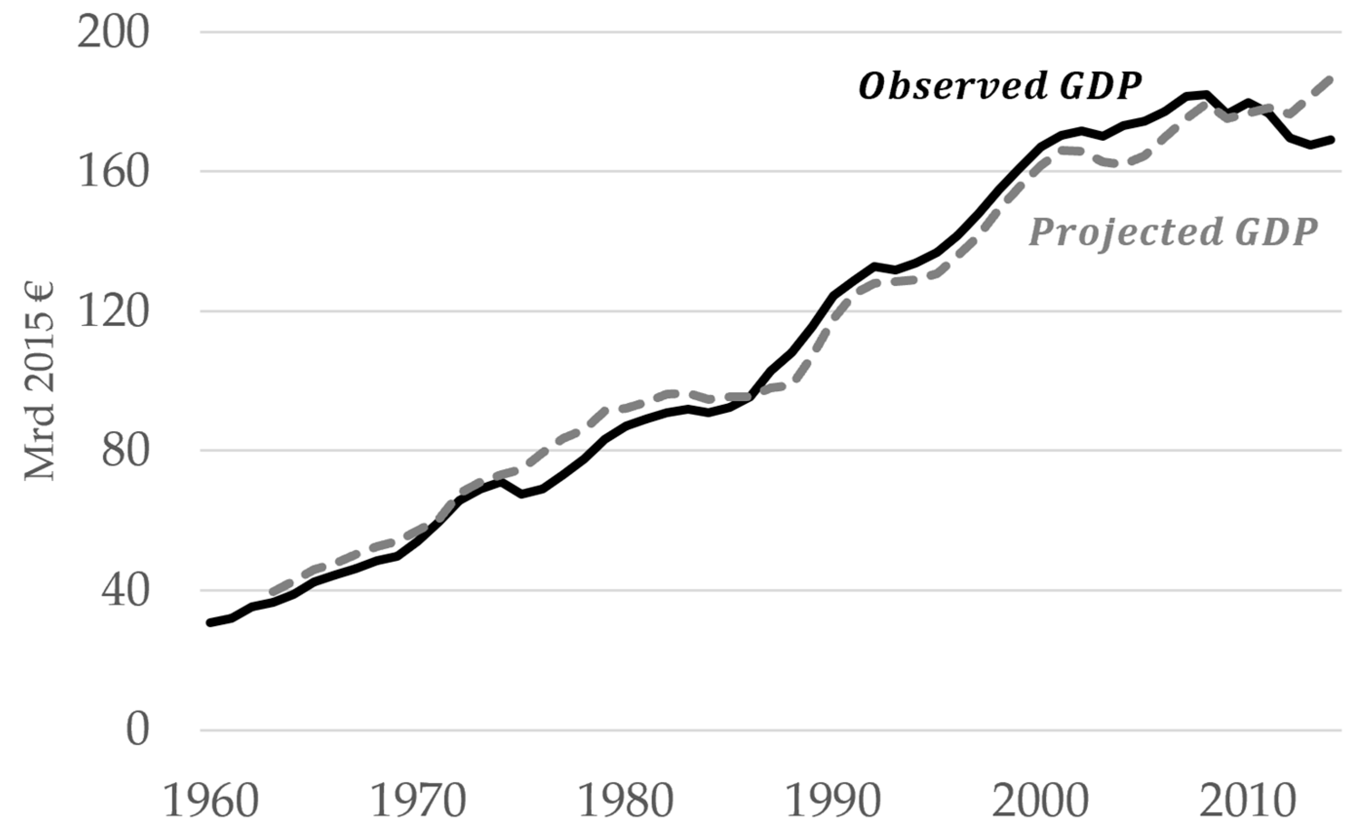
Figure 4 compares the actual values for economic output, or GDP ($Y$), and the basefit model solution of the MARCO-PT model for the same variable.

The basefit solution to the MARCO-PT model adequately replicates the historical economic output of the Portuguese economy 1960–2014. The same can be said for most other variables in the model—see Supplementary Materials (Section S5).

This first iteration of the MARCO-PT model generates good historical fits to observed data concerning the components of economic output, energy variables related to use ($FEN\_C$, $FEN\_IND$, $FEN\_OTH$, $UEX\_TOT$) and prices ($P\_EN\_C$, $P\_EN\_IND$, $P\_EN\_OTH$). Hence, the model is adequate to investigate the impact that changes in energy-related variables have had on historical economic growth.

4.3. Simulation Results and Output Elasticities

As described in Section 3.4, the impact of each selected variable on economic output is determined by an average output elasticity (Equation (10)).

Table 1. Average output elasticities for each selected variable in the Macroeconometric Resource Consumption model for Portugal (MARCO-PT) for whole period and subperiods. Values can be interpreted as % increase in economic output when selected variable increases by 1%. Green means a positive effect on economic output (dark green: elasticities above 0.5); red means a negative effect on economic output (dark red: elasticities below −0.1).

Scenario	Variable	Average Output Elasticity
		1965–1975	1976–1985	1986–1995	1996–2005	2006–2014	1965–2014
Scenario 1	Exergy efficiency	0.5434	0.5145	0.4797	0.4177	0.3028	0.4564
Scenario 2	Final energy	−0.0035	−0.0098	−0.0045	−0.0002	0.0006	−0.0036
Scenario 3	Investment	0.2683	0.2496	0.2648	0.2892	0.2435	0.2636
Scenario 4	Labor supply	−0.0339	−0.0457	−0.0792	−0.1792	−0.1822	−0.1011
Scenario 5	Energy prices	0.0135	0.0284	0.0372	0.0030	−0.0011	0.0165
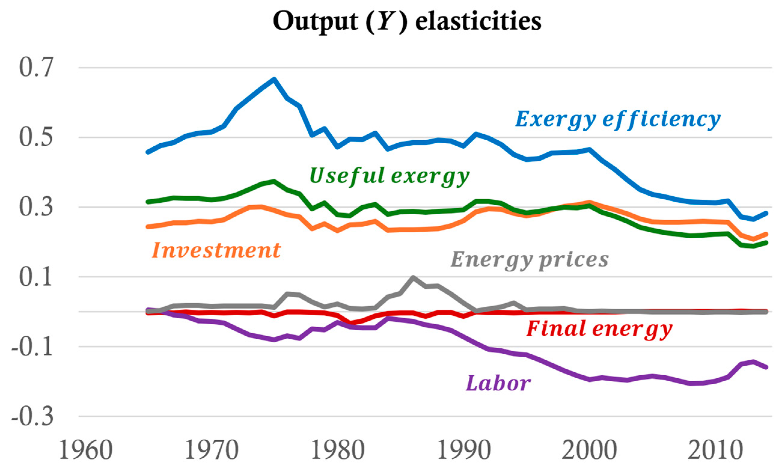
Scenario 6	Useful exergy	0.3345	0.3019	0.2959	0.2775	0.2118	0.2868

shows the average output elasticities computed for each of the six variables listed in Section 3.4 both for the overall period and the five subperiods of around 10 years each. The evolution of computed year-by-year output elasticities over time (Equation (9)) is represented in Figure 5. Due to the lagged terms in some of the stochastic equations, the initial value for all simulations, including the basefit solution, is 1965, not 1960.

Of the six variables selected for analysis in Section 3.4, the two largest historical influences on Portuguese GDP over the whole period 1965–2014 are: (1) aggregate thermodynamic final-to-useful exergy efficiency ($EXEFF\_FU$), with an average output elasticity of 0.46 (Figure 5, blue line); (2) total useful exergy consumption ($UEX\_TOT$), with an average output elasticity of 0.29 (Figure 5, green line). Investment expenditure in capital (I) is only the third largest overall historical influence, with an average output elasticity of 0.26 (Figure 5, orange line). Neither total final energy use ($FEN\_T$; Figure 5; red line) nor energy prices ($P\_EN\_C$, $P\_EN\_IND$, $P\_EN\_OTH$; Figure 5; grey line) have a significant impact on historical GDP (average output elasticities of less than 0.05 in absolute terms). On the other hand, labor supply growth is shown to have a negative impact on historical economic output 1965–2014 (average output elasticity −0.10; Figure 5; purple line).

The following subsections discuss these scenarios in detail, providing interpretation.

4.3.1. The Historical Impact of Energy Efficiency

The results shown in Figure 5 and Table 1 reveal several important findings concerning the role of energy in Portuguese historical economic growth.

The largest influence of growth, according to the average output elasticities computed for the whole period, is attributed to thermodynamic final-to-useful exergy efficiency. A 1% increase in this variable translates, on average, to a 0.46% increase in economic output. The second largest influence on growth is attributed to the quantity of useful exergy consumed in the economy. If the latter variable grows by 1%, an average 0.29% increase is expected in economic output. These results, by themselves, reveal the important role that energy—at the useful stage and measured by exergy content—has had on the Portuguese economy throughout the studied period. This finding is in line with the findings of the MARCO-UK model and supports the earlier modeling work of Robert Ayres and Benjamin Warr in their Resource-Exergy Services (REXS) model [46], where a significant role is evidenced for thermodynamic efficiency gains in US economic growth.

The importance of useful exergy consumption and thermodynamic final-to-useful energy efficiency to economic growth is even more evidenced when compared with the small impact estimated for either final energy consumed or energy prices. Increasing either by 1% leads to an expected average change in economic output close to 0%. Of all the energy-related variables considered in counterfactual simulations in this work, thermodynamic final-to-useful energy efficiency and total useful exergy consumed affect historical economic growth the most. This is also in line with the findings of the MARCO-UK model and provides additional support for assertions in the field of exergy economics that energy at the useful stage, in exergy terms, is more closely linked with economic growth [42,43,44,49,73,75,93,94]. As for the MARCO-UK model, the explicit inclusion of thermodynamic final-to-useful energy efficiency as an additional energy variable reduces the influence of final energy supply—and other explanatory variables—on growth.

From Table 1, we can see that thermodynamic final-to-useful exergy efficiency consistently exerts the largest influence on historical economic growth for all subperiods. Still, the largest average output elasticities for this variable (and total useful exergy consumed) are found in the earliest decades (1965–1985). This corresponds to the period of fastest GDP growth in the country. The earlier decades also correspond to the widespread electrification of the economy, corresponding to increases in overall efficiency and the possibility of delivering more useful exergy to production. The later decades saw a stagnation in final-to-useful exergy efficiency, mostly due to the proliferation of (less efficient) automobile utilization.

Both Table 1 and Figure 5 show that the output elasticities of thermodynamic final-to-useful exergy efficiency and total useful exergy consumption have been decreasing over time, particularly after the year 2000. This also occurs for the output elasticity of investment, and by the end of the period, these three variables have a similar positive influence on economic output.

4.3.2. Divergent Influences of Capital and Labor

The results presented in Table 1 and Figure 5 (orange and purple lines) reveal the estimated impact of the traditional inputs to production—investment in capital stock and human labor supply, respectively—on historical economic growth in Portugal.

Of the six studied variables in counterfactual simulations, investment in capital represents the third largest influence on historical economic growth, just below total useful exergy consumption. A 1% increase in capital investment is expected to produce, on average, a 0.26% increase in economic output. In the MARCO-UK model, capital investment is also identified as the third largest influence on the historical economic growth of the selected variables. From Figure 5 (orange line) and Table 1, the influence of capital investment on growth over time seems to be stable, as evidenced by its output elasticity changing little throughout the whole period.

Labor supply, on the other hand, is revealed to have an increasingly negative influence on historical economic growth, as shown by the negative, decreasing output elasticity for this variable. For the period as a whole, as labor supply grows by 1%, economic output is expected to decrease, on average, by 0.10%. Since 1995, the negative influence is even larger, with an average output elasticity closer to −0.2. The MARCO-PT framework is a post-Keynesian, demand-driven model and relies on a certain relation of substitutability between capital investment and human labor supply, by which labor shortage is compensated with additional capital investment to meet demand.

This is illustrated in Figure 6 (top right—dashed line), where the year-by-year capital investment elasticity of human labor is represented. A 1% increase in labor supply leads to a decrease in capital investment throughout the whole period, averaging −0.61%. Conversely, a 1% decrease in labor supply would, on average, result in an increase in capital investment of 0.61%, thus suggesting that the latter acts as a substitute for human labor in the MARCO-PT model: when labor supply goes down, capital investment goes up.

However, we cannot say that the relation of substitutability between capital investment and human labor works both ways. Looking at the year-by-year labor elasticity of capital investment—Figure 6 (top left—dashed line)—we see that it is positive for the whole period, albeit at a low, stable value of around 0.09. This means that a 1% decrease in capital investment would lead to, not an increase in human labor supply (as might be expected of substitute inputs to production), but a decrease of about 0.1% in human labor supply. Although small in magnitude, this behavior is more in line with complement inputs to production rather than substitutes.

Ultimately, this apparent contradiction concerning the substitutability or complementarity of capital investment and human labor may come down to if the labor supply is short, workers can work more hours and operate more capital to keep the same levels of production; if capital investment is short, increasing the number of workers will only lead to more engaged workers without capital to operate. In any case, these results support previous findings with the MARCO-UK model, namely that—of the two traditional inputs to production—human labor has a much lower effect than capital investment on economic growth.

On the other hand, the complementarity of traditional factors of production—capital and labor—with energy services (proxied by total useful exergy consumption) in the MARCO-PT model is suggested from observing Figure 6. Figure 6 (bottom) shows how the year-to-year total useful exergy elasticity of both capital investment and human labor supply is positive throughout the whole period, averaging 0.21 (capital investment—dashed line) and 0.39 (human labor—dotted line). Additionally, both capital investment elasticity of useful exergy and labor elasticity of useful exergy are positive throughout the whole period, averaging 0.17 in the case of labor (Figure 6 top left—dotted line) and 0.96 in the case of capital investment (Figure 6 top right—dotted line). This suggests that both capital and labor inputs to production require useful exergy flows to be put to work. An expansion of the capital stock through investment of fixed capital and/or an increase in labor, requires an increase in useful exergy. Steve Keen said it most eloquently: “labour without energy is a corpse, while capital without energy is a sculpture” [95] (p. 41).

4.4. Insights into the Role of Efficiency Energy Use on Economic Growth

Overall, the obtained results support the theoretical arguments and empirical findings from earlier work, particularly in the field of ecological economics (in the subfield of exergy economics).

First, previous studies have already posited that there is a tighter link between energy use and economic growth when useful exergy—the stage of quality-adjusted energy flows closest to energy services—is considered. Among these studies, we highlight the pioneering work of Robert Ayres and Benjamin Warr, in which the adoption of the useful exergy metric has improved modeling historical US economic growth [73] and evidence for causality from energy use to economic output [47]. We also highlight previous work that produced similar conclusions for the Portuguese economy [44,49] and other European countries [43]. In our work with the MARCO-PT model, we have evidenced how useful exergy and thermodynamic final-to-useful exergy efficiency had a larger historical influence on Portuguese economic growth than other—more standard—energy variables, such as final energy use or energy prices. Our results, therefore, support the argument that useful exergy is more closely connected to economic growth than other energy use variables.

Second, several studies have observed—following distinct methods—that the productive power of energy inputs (measured by their output elasticity) far outweighs their small share of costs. This is in direct contradiction with mainstream neoclassical growth models. We cite two of these studies: (1) a semi-parametric approach applied to 50 years of growth of 15 European countries [96]; (2) an unconventional parametric production function approach applied to Germany, Japan, and the US [97,98]. Both examples have in common the recognition that a thermodynamic approach is needed in modeling economic growth and adopting the useful exergy metric to account for productive energy uses. Our work with the MARCO-PT model corroborates their findings, with the historical influence of useful exergy and energy efficiency on growth being significantly larger than neoclassical theory assumes from its cost share. On the other hand, the MARCO-PT model projects the output elasticity of labor to be much smaller than its cost share, something that has also been previously evidenced in [97].

Third, as previous work has shown, improvements in the second law of thermodynamic energy conversion efficiency (i.e., final-to-useful exergy efficiency) have a great influence on economic growth. This has been uncovered by, among others, the work of [42] for the Portuguese economy, where a long-run statistically significant relationship is observed by which changes in the largest driver of economic growth—total factor productivity—are adequately proxied by changes in final-to-useful exergy efficiency. Our work with the MARCO-PT model finds, similarly, that changes in final-to-useful exergy efficiency have had a great positive impact on economic output for the past 50 years.

5. Conclusions

In this work, we develop and implement a thermodynamically consistent Macroeconometric Resource Consumption model for the Portuguese economy (MARCO-PT), capturing the complex interactions between macroeconomic, monetary, energy, and environmental variables.

Construction of the model is conducted by incorporating identities from national accounts and stochastic relationships—with short-run and long-run dynamics—evaluated and estimated using data for Portugal, 1960–2014. The outcome of this methodical and iterative process is an adequate projection of historical trends for endogenous variables in the model based on known exogenous variables. The model structure then allows for counterfactual (ex-post) simulations to be run, which, in turn, allow for computing year-by-year elasticities between variables of the model. Comparing the magnitude (and trend) of output elasticities for selected variables provides insights into the weight of each variable in influencing historically observed economic growth. In this sense, the analysis conducted here differs from that carried out with the UK counterpart (MARCO-UK) of the proposed model. Rather than running counterfactual simulations holding one variable constant for a period of 50 years—which may push the model outside of its calibrated space—we opt to test the immediate annual effect of each variable on output. While the two methods differ in their approach, our results for the Portuguese economy support the findings for the UK.

Average output elasticities for the six selected variables in our work reveal that the two largest historical influences on economic growth can be attributed to: (1) thermodynamic final-to-useful energy efficiency (average output elasticity 0.46); (2) total useful exergy consumed (average output elasticity 0.29). The influence of these two variables on growth is larger than either more conventional energy variables (total final energy consumed or energy prices) or the traditional factors of production (capital investment and human labor supply). On average, a 1% increase in thermodynamic final-to-useful energy efficiency leads to a percentage growth in GDP that is 1.5 times that of a comparable increase in capital investment.

While always positive, the influence of thermodynamic final-to-useful energy efficiency is not the same throughout the whole period 1965–2014. It is higher (average output elasticities 0.50–0.55) in earlier decades (1965–1985) and declines in later years (average output elasticity 0.30 between 2005–2014). This might be due to the transition to a service-based economy, but further investigation is warranted. Despite this drop, it consistently has the largest influence on growth throughout the whole 50-year period. The period of highest average output elasticity of thermodynamic efficiency coincides with the period of fastest growth of GDP in the Portuguese economy. Mainstream neoclassical approaches to growth theory attribute this increase in GDP to an increase in exogenous total factor productivity and attempt to explain it with abstract considerations of technological and/or institutional change while neglecting the role of energy. In contrast, the MARCO-PT model offers a thermodynamically consistent approach to describe historical economic growth.

Concerning the traditional factors of production, results from our analysis reveal divergent influences on economic growth. Capital investment plays, as expected, a strong role in the economy, with an average output elasticity of 0.26 (third largest of studied variables—almost tied with supply of useful exergy). This influence is also stable throughout the whole 50-year period. Capital investment also seems to be able to act as a substitute for human labor supply, perhaps justifying the small (and negative) influence that the latter has on economic growth. Useful exergy supply seems to behave as a complement to both capital investment and human labor supply.

The aforementioned results have important implications for economic growth modeling, particularly for growth scenarios incorporated in IAMs that inform climate change policies. Given the size of the contributions of useful stage exergy and efficiency to economic growth, it is imperative that such models become thermodynamically consistent. The economic growth models embedded in IAM generating IPCC’s scenarios often assume high capital-energy substitutability. This is only one of the many issues surrounding the modeling choices with constant elasticity of substitution (CES) production functions adopted in these models [99]. The implication is that the scenarios assume that absolute energy decoupling is both readily feasible and inexpensive [100]. While reducing energy demand is a key mechanism for emission reduction, the implications for economic growth of reducing energy demand are insufficiently explored in IAMs. Also, none of these models adequately include rebound effects [101], which are poorly understood at the macroeconomic level but could be substantial. Thermodynamically consistent modeling, such as shown in this work with the MARCO-PT model, constitutes a step towards a better understanding of the role of energy in the economy—both a driver and a constraint—and consider the best policy response.

Thinking about the future, the MARCO model is a versatile framework, having been adopted for different research and policy purposes in the UK [102]. The framework is also undergoing constant revision and improvement, aiming for: (a) added granularity—splitting sectors into subsectors and distinguishing between renewable and non-renewable energy inputs; (b) introducing additional constraints and feedback loops—e.g., financial and labor availability constraints, etc.; (c) inclusion of transport and Information and Communication Technologies (ICT). For Portugal, the model is currently being adapted to study the socio-macroeconomic impacts of implementing various energy policy measures put forward by the Portuguese Environmental Agency. The MARCO model can be implemented for other countries, thereby confirming the results obtained so far and/or identifying the idiosyncrasies of different countries.

References

1. IEA. Capturing the Multiple Benefits of Energy Efficiency; IEA: Paris, France, 2015; Available online: https://www.iea.org/reports/capturing-the-multiple-benefits-of-energy-efficiency (accessed on 14 September 2023).
2. Dean, E.; Harper, M. The BLS productivity measurement program. In New Developments in Productivity Analysis; University of Chicago Press: Chicago, IL, USA, 2001; pp. 55–84. [Google Scholar]
3. Feenstra, R.C.; Inklaar, R.; Timmer, M.P. The Next Generation of the Penn World Table. Am. Econ. Rev. 2015, 105, 3150–3182. [Google Scholar] [CrossRef]
4. Schreyer, P.; Pilat, D. Measuring productivity. OECD Econ. Stud. 2001, 33, 127–170. [Google Scholar]
5. Timmer, M.P.; O’Mahony, M.; Van Ark, B. EU KLEMS growth and productivity accounts: An overview. Int. Product. Monit. 2007, 14, 74–85. [Google Scholar] [CrossRef]
6. Easterly, W.; Levine, R. What have we learned from a decade of empirical research on growth? It’s Not Factor Accumulation: Stylized Facts and Growth Models. World Bank Econ. Rev. 2001, 15, 177–219. [Google Scholar] [CrossRef]
7. Acs, Z.J.; Estrin, S.; Mickiewicz, T.; Szerb, L. The Continued Search for the Solow Residual: The Role of National Entrepreneurial Ecosystem (No. 8652). IZA Discussion Papers. 2014. Available online: https://www.iza.org/publications/dp/8652/the-continued-search-for-the-solow-residual-the-role-of-national-entrepreneurial-ecosystem (accessed on 17 April 2023).
8. Solow, R.M. Technical progress, capital formation, and economic growth. Am. Econ. Rev. 1962, 52, 76–86. [Google Scholar]
9. Denison, E.F. Education, economic growth, and gaps in information. J. Political Econ. 1962, 70, 124–128. [Google Scholar] [CrossRef]
10. Denison, E.F. Sources of postwar growth in nine western countries. Am. Econ. Rev. 1967, 57, 325–332. [Google Scholar]
11. Jorgenson, D.W.; Griliches, Z. The explanation of productivity change. Rev. Econ. Stud. 1967, 34, 249–283. [Google Scholar] [CrossRef]
12. Acemoglu, D.; Dell, M. Productivity differences between and within countries. Am. Econ. J. Macroecon. 2010, 2, 169–188. [Google Scholar] [CrossRef]
13. Oulton, N. The Mystery of TFP; CFM Discussion Paper Series (CFM-DP2017-06); Centre For Macroeconomics: London, UK, 2016; p. 31. [Google Scholar]
14. O’Mahony, M.; Castaldi, C.; Los, B.; Bartelsman, E.; Maimaiti, Y.; Peng, F. EUKLEMS-Linked Data: Sources and Methods; University of Birmingham: Birmingham, UK, 2008. [Google Scholar]
15. Koszerek, D.; Havik, K.; Mc Morrow, K.; Röger, W.; Schönborn, F. An Overview of the EU KLEMS Growth and Productivity Accounts. European Economy-Economic Papers 2008–2015 Number 290. 2007. Available online: https://ec.europa.eu/economy_finance/publications/pages/publication9467_en.pdf (accessed on 2 November 2023).
16. Van Ark, B. Total Factor Productivity: Lessons from the Past and Directions for the Future (No. 271). NBB Working Paper. 2014. Available online: https://www.nbb.be/doc/ts/publications/wp/wp271en.pdf (accessed on 24 May 2023).
17. Felipe, J.; McCombie, J.S. How sound are the foundations of the aggregate production function? East. Econ. J. 2005, 31, 467–488. [Google Scholar]
18. Felipe, J.; McCombie, J.S. The aggregate production function: “Not even wrong”. Rev. Political Econ. 2014, 26, 60–84. [Google Scholar] [CrossRef]
19. McCombie, J.S. What does the aggregate production function show? Further thoughts on Solow’s “second thoughts on growth theory”. J. Post Keynes. Econ. 2001, 23, 589–615. [Google Scholar] [CrossRef]
20. Sraffa, P. Production of commodities by means of commodities. In What Are the Questions and Other Essays; Routledge: London, UK, 2016; pp. 144–150. [Google Scholar]
21. Robinson, J. The production function and the theory of capital. Rev. Econ. Stud. 1953, 21, 81–106. [Google Scholar] [CrossRef]
22. King, J.E. A History of Post Keynesian Economics Since 1936; Edward Elgar Publishing: Cheltenham, UK, 2002. [Google Scholar]
23. Kim, Y.E.; Loayza, N. Productivity growth: Patterns and determinants across the world. In World Bank Policy Research Working Paper 8852; World Bank: Washington, DC, USA, 2019. [Google Scholar]
24. Stanton, E.A.; Ackerman, F.; Kartha, S. Inside the integrated assessment models: Four issues in climate economics. Clim. Dev. 2009, 1, 166–184. [Google Scholar] [CrossRef]
25. Millner, A.; McDermott, T.K. Model confirmation in climate economics. Proc. Natl. Acad. Sci. USA 2016, 113, 8675–8680. [Google Scholar] [CrossRef] [PubMed]
26. Daly, H.E. When smart people make dumb mistakes. Ecol. Econ. 2000, 34, 1–3. [Google Scholar] [CrossRef]
27. Solow, R.M. Intergenerational equity and exhaustible resources. Rev. Econ. Stud. 1974, 41, 29–45. [Google Scholar] [CrossRef]
28. Stiglitz, J. Growth with exhaustible natural resources: Efficient and optimal growth paths. Rev. Econ. Stud. 1974, 41, 123–137. [Google Scholar] [CrossRef]
29. Hudson, E.A.; Jorgenson, D.W. Energy policy and US economic growth. Am. Econ. Rev. 1978, 68, 118–123. [Google Scholar]
30. Allen, E.L.; Cooper, C.L.; Edmonds, F.C.; Edmonds, J.A.; Reister, D.B.; Weinberg, A.M.; Whittle, C.E.; Zelby, L.W. US Energy and Economic Growth, 1975–2010; No. ORAU/IEA-76-7; Institute for Energy Analysis: Oak Ridge, TN, USA, 1976. [Google Scholar] [CrossRef]
31. Jorgenson, D.W. The role of energy in the US economy. Natl. Tax J. 1978, 31, 209–220. [Google Scholar] [CrossRef]
32. Koetse, M.J.; De Groot, H.L.; Florax, R.J. Capital-energy substitution and shifts in factor demand: A meta-analysis. Energy Econ. 2008, 30, 2236–2251. [Google Scholar] [CrossRef]
33. Fiorito, G.; van den Bergh, J.C. Capital-energy substitution in manufacturing for seven OECD countries: Learning about potential effects of climate policy and peak oil. Energy Effic. 2016, 9, 49–65. [Google Scholar] [CrossRef]
34. d’Arge, R.C.; Kogiku, K.C. Economic growth and the environment. Rev. Econ. Stud. 1973, 40, 61–77. [Google Scholar] [CrossRef]
35. Kümmel, R. Energy as a factor of production and entropy as a pollution indicator in macroeconomic modelling. Ecol. Econ. 1989, 1, 161–180. [Google Scholar] [CrossRef]
36. Gross, L.S.; Veendorp, E.C.H. Growth with Exhaustible Resources and a Materials-Balance Production Function. Nat. Resour. Model. 1990, 4, 77–94. [Google Scholar] [CrossRef]
37. Lindenberger, D.; Kümmel, R. Energy and the state of nations. Energy 2011, 36, 6010–6018. [Google Scholar] [CrossRef]
38. Dincer, I.; Rosen, M.A. Exergy: Energy, Environment and Sustainable Development; Newnes: Oxford, UK, 2012. [Google Scholar]
39. Reistad, G.M. Available energy conversion and utilization in the United States. ASME J. Eng. Power 1975, 97, 429–434. [Google Scholar] [CrossRef]
40. APS. Energy Future: Think Efficiency: How America Can Look within to Achieve; American Physical Society: Washington, DC, USA, 2008. [Google Scholar]
41. Cullen, J.M.; Allwood, J.M.; Borgstein, E.H. Reducing energy demand: What are the practical limits? Environ. Sci. Technol. 2011, 45, 1711–1718. [Google Scholar] [CrossRef] [PubMed]
42. Santos, J.; Borges, A.S.; Domingos, T. Exploring the links between total factor productivity and energy efficiency: Portugal, 1960–2014. Energy Econ. 2021, 101, 105407. [Google Scholar] [CrossRef]
43. Serrenho, A.C.; Sousa, T.; Warr, B.; Ayres, R.U.; Domingos, T. Decomposition of useful work intensity: The EU (European Union)-15 countries from 1960 to 2009. Energy 2014, 76, 704–715. [Google Scholar] [CrossRef]
44. Serrenho, A.C.; Warr, B.; Sousa, T.; Ayres, R.U.; Domingos, T. Structure and dynamics of useful work along the agriculture-industry-services transition: Portugal from 1856 to 2009. Struct. Chang. Econ. Dyn. 2016, 36, 1–21. [Google Scholar] [CrossRef]
45. Sousa, T.; Brockway, P.E.; Cullen, J.M.; Henriques, S.T.; Miller, J.; Serrenho, A.C.; Domingos, T. The need for robust, consistent methods in societal exergy accounting. Ecol. Econ. 2017, 141, 11–21. [Google Scholar] [CrossRef]
46. Warr, B.; Ayres, R. REXS: A forecasting model for assessing the impact of natural resource consumption and technological change on economic growth. Struct. Chang. Econ. Dyn. 2006, 17, 329–378. [Google Scholar] [CrossRef]
47. Warr, B.S.; Ayres, R.U. Evidence of causality between the quantity and quality of energy consumption and economic growth. Energy 2010, 35, 1688–1693. [Google Scholar] [CrossRef]
48. Warr, B.; Ayres, R.U. Useful work and information as drivers of economic growth. Ecol. Econ. 2012, 73, 93–102. [Google Scholar] [CrossRef]
49. Santos, J.; Domingos, T.; Sousa, T.; Aubyn, M.S. Useful exergy is key in obtaining plausible aggregate production functions and recognizing the role of energy in economic growth: Portugal 1960–2009. Ecol. Econ. 2018, 148, 103–120. [Google Scholar] [CrossRef]
50. Sakai, M.; Brockway, P.E.; Barrett, J.R.; Taylor, P.G. Thermodynamic efficiency gains and their role as a key ‘engine of economic growth’. Energies 2019, 12, 110. [Google Scholar] [CrossRef]
51. Wall, G. Exergy conversion in the Swedish society. Resour. Energy 1987, 9, 55–73. [Google Scholar] [CrossRef]
52. Sciubba, E. Beyond thermoeconomics? The concept of extended exergy accounting and its application to the analysis and design of thermal systems. Exergy Int. J. 2001, 1, 68–84. [Google Scholar] [CrossRef]
53. Heun, M.K.; Brockway, P.E. Meeting 2030 primary energy and economic growth goals: Mission impossible? Appl. Energy 2019, 251, 112697. [Google Scholar] [CrossRef]
54. European Commission. Assessing the Employment and Social Impact of Energy Efficiency, Report Submitted to the European Commission (DG ENER) by Cambridge Econometrics, E3MLab, ICF International and Warwick Institute for Employment Research. 2015. Available online: https://ec.europa.eu/energy/sites/ener/files/documents/CE_EE_Jobs_main18Nov2015.pdf (accessed on 30 July 2023).
55. European Commission. A Spatial Computable General Equilibrium Model for EU Regions and Sectors. 2016. Available online: https://ec.europa.eu/jrc/en/publication/rhomolo-v2-model-description-spatial-computable-general-equilibrium-model-eu-regions-and-sectors (accessed on 1 December 2023).
56. HRMC. Technical Documents and Research Based on HM Revenue & Customs (HRMC) CGE Model. 2013. Available online: https://www.gov.uk/government/publications/computable-general-equilibrium-cge-modelling (accessed on 22 February 2023).
57. OBR. The Macroeconomic Model. Briefing Paper No. 5. 2013. Available online: https://budgetresponsibility.org.uk/topics/obr-macroeconomic-model/ (accessed on 1 April 2023).
58. Geanakoplos, J. Arrow-Debreu Model of General Equilibrium; Palgrave Macmillan: London, UK, 1989; pp. 43–61. [Google Scholar]
59. Babatunde, K.A.; Begum, R.A.; Said, F.F. Application of computable general equilibrium (CGE) to climate change mitigation policy: A systematic review. Renew. Sustain. Energy Rev. 2017, 78, 61–71. [Google Scholar] [CrossRef]
60. Sterman, J.; Fiddaman, T.; Franck, T.; Jones, A.; McCauley, S.; Rice, P.; Sawin, E.; Siegel, L. Climate interactive: The C-ROADS climate policy model. Syst. Dyn. Rev. 2012, 28, 295–305. [Google Scholar] [CrossRef]
61. ENE (Environment Northeast). Energy Efficiency: Engine of Economic Growth in Eastern Canada. A Macroeconomic Modeling & Tax Revenue Impact Assessment, ENE Ottawa. 2012. Available online: www.env-ne.org/public/resources/ENE_EnergyEfficiencyEngineofEconomicGrowth_EarternCanada_EN_2012_0611_FINAL.pdf (accessed on 8 January 2023).
62. Pollitt, H.; Lewney, R.; Mercure, J.F. Conceptual differences between macro-econometric and CGE models. In Proceedings of the 27th International Input-Output Association Conference, Glasgow, UK, 30 June–5 July 2019. [Google Scholar]
63. Barker, T.; Anger, A.; Chewpreecha, U.; Pollitt, H. A new economics approach to modelling policies to achieve global 2020 targets for climate stabilisation. Int. Rev. Appl. Econ. 2012, 26, 205–221. [Google Scholar] [CrossRef]
64. Lavoie, M. Post-Keynesian Economics: New Foundations; Edward Elgar Publishing: Cheltenham, UK, 2022. [Google Scholar]
65. Scrieciu, S.; Rezai, A.; Mechler, R. On the economic foundations of green growth discourses: The case of climate change mitigation and macroeconomic dynamics in economic modeling. Wiley Interdiscip. Rev. Energy Environ. 2013, 2, 251–268. [Google Scholar] [CrossRef]
66. Patterson, M.G. What is energy efficiency?: Concepts, indicators and methodological issues. Energy Policy 1996, 24, 377–390. [Google Scholar] [CrossRef]
67. Madlener, R.; Alcott, B. Energy rebound and economic growth: A review of the main issues and research needs. Energy 2009, 34, 370–376. [Google Scholar] [CrossRef]
68. Van der Werf, E. Production functions for climate policy modeling: An empirical analysis. Energy Econ. 2008, 30, 2964–2979. [Google Scholar] [CrossRef]
69. Mundaca, L.; Neij, L.; Worrell, E.; McNeil, M. Evaluating energy efficiency policies with energy-economy models. Annu. Rev. Environ. Resour. 2010, 35, 305–344. [Google Scholar] [CrossRef]
70. E3ME Technical Manual; Version 6; Cambridge Econometrics: Cambridge, UK, 2014.
71. Sijm, J.; Lehmann, P.; Chewpreecha, U.; Gawel, E.; Mercure, J.F.; Pollitt, H.; Strunz, S. EU Climate and Energy Policy beyond 2020: Are Additional Targets and Instruments for Renewables Economically Reasonable? In The European Dimension of Germany’s Energy Transition; (No. 3/2014), UFZ Discussion Paper; Springer: Cham, Switzerland, 2014. [Google Scholar]
72. Ertesvåg, I.S. Society exergy analysis: A comparison of different societies. Energy 2001, 26, 253–270. [Google Scholar] [CrossRef]
73. Ayres, R.U.; Warr, B. Accounting for growth: The role of physical work. Struct. Chang. Econ. Dyn. 2005, 16, 181–209. [Google Scholar] [CrossRef]
74. Stresing, R.; Lindenberger, D.; Kümmel, R. Cointegration of output, capital, labor, and energy. Eur. Phys. J. B 2008, 66, 279–287. [Google Scholar] [CrossRef]
75. Guevara, Z.; Sousa, T.; Domingos, T. Insights on energy transitions in Mexico from the analysis of useful exergy 1971–2009. Energies 2016, 9, 488. [Google Scholar] [CrossRef]
76. Felício, L.; Henriques, S.T.; Serrenho, A.; Domingos, T.; Sousa, T. Insights from past trends in exergy efficiency and carbon intensity of electricity: Portugal, 1900–2014. Energies 2019, 12, 534. [Google Scholar] [CrossRef]
77. Brillet, J.L. Structural Econometric Modelling: Methodology and Tools with Applications under EViews; IHS Global Inc.: Englewood, CO, USA, 2016. [Google Scholar]
78. Johansen, S. Statistical analysis of cointegration vectors. J. Econ. Dyn. Control 1988, 12, 231–254. [Google Scholar] [CrossRef]
79. Dickey, D.A.; Fuller, W.A. Likelihood ratio statistics for autoregressive time series with a unit root. Econom. J. Econom. Soc. 1981, 49, 1057–1072. [Google Scholar] [CrossRef]
80. Phillips, P.C.; Perron, P. Testing for a unit root in time series regression. Biometrika 1988, 75, 335–346. [Google Scholar] [CrossRef]
81. [database] AMECO. Annual Macro-Economic Database of the European Commission’s Directorate General for Economic and Financial Affairs. 2022. Available online: https://economy-finance.ec.europa.eu/economic-research-and-databases/economic-databases/ameco-database_en (accessed on 13 January 2023).
82. [database] DGEG. Direção-Geral de Energia e Geologia. Estatísticas e Preços—Estatística da Energia. 2023. Available online: http://www.dgeg.gov.pt/ (accessed on 13 January 2023).
83. [database] Banco de Portugal. Novas Séries Longas Para A Economia Portuguesa—SLEP2020. Portal de estatísticas do Banco de Portugal. 2020. Available online: https://bpstat.bportugal.pt/conteudos/noticias/1498/ (accessed on 13 January 2023).
84. [database] EuroStat. European Statistics Database. 2023. Available online: https://ec.europa.eu/eurostat/data/database (accessed on 13 January 2023).
85. [database] World Bank. World Development Indicator. World Bank National Accounts Data, and OECD National Accounts Data Files. 2023. Available online: https://data.worldbank.org/indicator/ (accessed on 13 January 2023).
86. [database] Global Carbon Atlas. Portugal—Territorial (MtCO2). 2018. Available online: http://www.globalcarbonatlas.org/en/CO2-emissions (accessed on 13 January 2023).
87. da Silva, E.G.; Lains, P. Capital Formation and Long-Run Growth: Evidence from Portuguese Data, 1910–2011; IBEROMETRICS VI; Facultad de Economía y Empresa: Zaragoza, Spain, 2013; pp. 16–17. [Google Scholar]
88. Varga, R.S. Basic Iterative Methods and Comparison Theorems. In Matrix Iterative Analysis; Springer: Berlin/Heidelberg, Germany, 2009; pp. 63–110. [Google Scholar]
89. Koesler, S.; Swales, K.; Turner, K. International spillover and rebound effects from increased energy efficiency in Germany. Energy Econ. 2016, 54, 444–452. [Google Scholar] [CrossRef]
90. Allan, G.; Gilmartin, M.; Turner, K.; McGregor, P.G.; Swales, J.K. UKERC Review of Evidence for the Rebound Effect: Technical Report 4: Computable General Equilibrium Modelling Studies. 2007. Available online: https://ukerc.ac.uk/publications/ukerc-review-of-evidence-for-the-rebound-effect-technical-report-4-computable-general-equilibrium-modelling-studies/ (accessed on 14 September 2023).
91. Froot, K.A.; Rogoff, K. Perspectives on PPP and long-run real exchange rates. Handb. Int. Econ. 1995, 3, 1647–1688. [Google Scholar]
92. Sercu, P.; Uppal, R.; Van Hulle, C. The exchange rate in the presence of transaction costs: Implications for tests of purchasing power parity. J. Financ. 1995, 50, 1309–1319. [Google Scholar] [CrossRef]
93. Brockway, P.E.; Barrett, J.R.; Foxon, T.J.; Steinberger, J.K. Divergence of trends in US and UK aggregate exergy efficiencies 1960–2010. Environ. Sci. Technol. 2014, 48, 9874–9881. [Google Scholar] [CrossRef]
94. Brockway, P.; Sorrell, S.; Foxon, T.; Miller, J. Exergy economics: New insights into energy consumption and economic growth. In Transitions in Energy Efficiency and Demand; Routledge: London, UK, 2018; pp. 133–155. [Google Scholar]
95. Keen, S.; Ayres, R.U.; Standish, R. A Note on the Role of Energy in Production. Ecol. Econ. 2019, 157, 40–46. [Google Scholar] [CrossRef]
96. Voudouris, V.; Ayres, R.; Serrenho, A.C.; Kiose, D. The economic growth enigma revisited: The EU-15 since the 1970s. Energy Policy 2015, 86, 812–832. [Google Scholar] [CrossRef]
97. Kümmel, R.; Lindenberger, D.; Weiser, F. The economic power of energy and the need to integrate it with energy policy. Energy Policy 2015, 86, 833–843. [Google Scholar] [CrossRef]
98. Kümmel, R.; Ayres, R.U.; Lindenberger, D. Thermodynamic laws, economic methods and the productive power of energy. J. Non-Equilibrium Thermodyn. 2010, 35, 145–179. [Google Scholar] [CrossRef]
99. Heun, M.K.; Santos, J.; Brockway, P.E.; Pruim, R.; Domingos, T.; Sakai, M. From theory to econometrics to energy policy: Cautionary tales for policymaking using aggregate production functions. Energies 2017, 10, 203. [Google Scholar] [CrossRef]
100. Semieniuk, G.; Taylor, L.; Rezai, A.; Foley, D.K. Plausible energy demand patterns in a growing global economy with climate policy. Nat. Clim. Chang. 2021, 11, 313–318. [Google Scholar] [CrossRef]
101. Brockway, P.E.; Sorrell, S.; Semieniuk, G.; Heun, M.K.; Court, V. Energy efficiency and economy-wide rebound effects: A review of the evidence and its implications. Renew. Sustain. Energy Rev. 2021, 141, 110781. [Google Scholar] [CrossRef]
102. Nieto, J.; Pollitt, H.; Brockway, P.E.; Clements, L.; Sakai, M.; Barrett, J. Socio-macroeconomic impacts of implementing different post-Brexit UK energy reduction targets to 2030. Energy Policy 2021, 158, 112556. [Google Scholar] [CrossRef]
103. FRED. Federal Reserve Bank of St. Louis. Consumer Price Index: Energy for Portugal [PRTCPIENGAINMEI]. 2019. Available online: https://fred.stlouisfed.org/series/PRTCPIENGAINMEI (accessed on 13 January 2023).
Figure 1. Primary-to-final-to-useful energy/exergy conversion stages. Adapted from [42].
Energies 17 02688 g001
Figure 2. Simplified schematics for the Macroeconometric Resource Consumption model for Portugal (MARCO-PT) model structure. Adapted from [50].
Energies 17 02688 g002
Figure 3. Flowchart for estimation of individual stochastic equations in the Macroeconometric Resource Consumption model for Portugal (MARCO-PT) model, based on the stochastic equations of the MARCO UK model. SR indicates equations with only short-run dynamics (VAR). SR + LR indicate equations with both short-run and long-run dynamics (VECM). ECT stands for error-correction term.
Energies 17 02688 g003
Figure 4. Basefit simulation for gross domestic product (GDP) in Macroeconometric Resource Consumption model for Portugal (MARCO-PT). Economic output (real GDP) for the Portuguese economy 1960–2014, as observed historical values (full black line) and projected basefit solution from the MARCO-PT model (grey dashed line).
Energies 17 02688 g004
Figure 5. Year-by-year output elasticities for selected variables in the Macroeconometric Resource Consumption model for Portugal (MARCO-PT). Blue—thermodynamic final-to-useful exergy efficiency (EXEFF_FU); red—total final energy use (FEN_T); orange—investment (I); purple—labor supply (L); grey—energy prices (P_EN_C, P_EN_IND, P_EN_OTH); green—total useful exergy use (UEX_TOT).
Energies 17 02688 g005
Figure 6. Year-by-year elasticities between selected variables in the Macroeconometric Resource Consumption model for Portugal (MARCO-PT). Top left: human labor ( L ) elasticities of capital investment ( I )—dashed line and of total useful exergy ( U E X _ T O T )—dotted line. Top right: capital investment ( I ) elasticities of human labor ( L )—dashed line and of total useful exergy ( U E X _ T O T )—dotted line. Bottom: total useful exergy ( U E X _ T O T ) elasticities of capital investment ( I )—dashed line and of human labor ( L )—dotted line.
Energies 17 02688 g006