Abstract
This study addresses the challenges faced by coal-fired power plants in adapting to energy fluctuations following the integration of renewable energy sources into the power grid. The flexible operation of thermal power plants has become a focal point in academic research. A numerical model of a coal-fired power plant was developed in this study using the Long Short-Term Memory (LSTM) algorithm and the Particle Swarm Optimization (PSO) algorithm based on actual operation data analysis. The combined PSO-LSTM approach improved the accuracy of the model by optimizing parameters. Validation of the model was performed using a Dymola physical simulation model, demonstrating that the PSO-LSTM coupled numerical model accurately simulates coal-fired power plant operations with a goodness of fit reaching 0.998. Overall system performance for comprehensively evaluating the rate and accuracy of unit operation is proposed. Furthermore, the model’s capability to simulate the load variation process of automatic generation control (AGC) under different load command groups was assessed, aiding in optimizing the best load command group. Optimization experiments show that the performance index of output power is optimal within the experimental range when the set load starts and stops are the same and the power of load command γ = 1.8. Specifically, the 50–75% Turbine Heat Acceptance (THA) load rise process enhanced the overall system performance index by 55.1%, while the 75–50% THA load fall process improved the overall system performance index by 54.2%. These findings highlight the effectiveness of the PSO-LSTM approach in optimizing thermal power plant operations and enhancing system performance under varying load conditions.
1. Introduction
The adoption of the “peak carbon and carbon neutral” objective during the 75th session of the United Nations General Assembly and subsequent reaffirmations at the World Summit on Climate Ambition have established a global commitment to reducing carbon emissions [1]. Projections indicate that by 2030 there will be a minimum 65 percent reduction in global carbon dioxide emissions per unit of GDP compared to 2005 levels, with non-fossil fuels comprising at least 25 percent of primary energy consumption [2]. This transition will involve wind, solar, and other emerging energy sources contributing to a total installed capacity of 1.2 billion kilowatts worldwide [3].
As of the end of 2020, China has demonstrated significant momentum in the development of new energy sources, boasting an installed wind power capacity of 280 million kilowatts and solar power capacity of 250 million kilowatts. Experts estimate that within the next decade, China’s combined installed wind and solar power capacity will exceed 670 million kilowatts, accounting for approximately 33 percent of the nation’s total power generation capacity as of 2019 [4]. However, renewable energy sources, despite their growth, present challenges in meeting electricity demand during certain periods due to their inherent intermittency [5].
Consequently, the responsibility of ensuring clean energy consumption primarily falls upon thermal power units, which offer large installed capacities, high stability, and mature technology [6]. Given the substantial integration of renewable energy into the grid, thermal power units face a formidable task in accommodating the additional demand for new energy consumption [7].
With the widespread integration of renewable energy into the grid, the power system is undergoing significant transformations across various aspects such as stabilization mechanisms, dispatch operations, and planning development [8]. In recent years, the challenge of domestic power dispatch has gradually surfaced, with the core issue revolving around addressing the spatial and temporal uncertainties stemming from the intermittency of renewable energy sources [9]. Currently, this challenge is primarily managed by thermal power units, which possess large installed capacities, high stability, and mature technologies [10]. However, as various types of new energy units and distributed clean energy technologies rapidly develop, the dominance of thermal power units in providing heating services restricts their regulatory capacity, further deepening the integration of energy coupling and information interaction between the power and heating systems [11].
Power system flexibility, crucial for addressing supply and demand fluctuations and uncertainties in a stable, reliable, and cost-effective manner within specific timeframes, underscores the importance of enhancing the flexible operation capabilities of thermal power units in China’s energy structure transformation and development [12]. Presently, thermal power units typically operate at as low as 30–40% of their rated load during deep grid peaking, indicating limited flexibility [13]. Moreover, the presence of numerous cogeneration units within thermal power plants constrains the acceptance of new energy power during heating periods, intensifying the complexity of renewable energy consumption [14].
To address these challenges, numerous experts and scholars have conducted research on the variable load operations of thermal power units. For instance, Luo Qing et al. [15] developed a dynamic model of boiler heat exchangers under variable load conditions. Their objective was to investigate the dynamic response characteristics of each heating surface of the boiler when subjected to step changes in various boundary conditions. Zhao Yongliang et al. [16] utilized GSE software to model the automatic generation control (AGC) variable load process of a thermal power unit. Their study focused on analyzing the variations in key parameters of the thermal power unit during the variable load operations. Additionally, Zlatkovikj et al. [17] employed Dymola 2022x software to simulate biomass cogeneration boilers, thereby enhancing the control efficacy of the boilers under variable operating conditions
Currently, the primary technical approaches to enhancing the low-load stable combustion capability of thermal power units involve adjustments to the wind–coal ratio and modifications to the operational control mode of coal mills [18]. However, implementing these adjustments is often challenging based solely on theoretical understanding and operational experience.
With the advancement and utilization of technologies such as big data analysis, various industries in China are undergoing rapid digitalization and intelligence-driven transformations, unlocking the latent value embedded within data [19]. In recent years, machine learning, deep learning, and other advanced algorithms have found widespread application in the energy sector, particularly in optimizing control systems and predicting key parameters [20,21].
For instance, Si RuiCai et al. [22] developed a high, medium, and low-load model for a 600 MW thermal power unit using a back propagation (BP) neural network to enhance unit control processes. Additionally, Zhang GuangMing et al. [23] introduced a data-driven unit modeling approach based on the MLP algorithm, alongside an offline reinforcement learning-based coordinated control method for electricity and heat.
In summary, numerous scholars and experts have dedicated efforts to optimizing control systems to enhance the flexibility of thermal power units [24,25]. The primary challenge lies in managing parameter fluctuations during the unit’s variable load operations, particularly in deep peaking scenarios [26]. This necessitates the development of models for thermal unit operation and control processes, often relying on simulation software or individual intelligent algorithms [27].
The optimization of load instructions for coal-fired units holds paramount importance. By effectively managing and adjusting load instructions, these units can enhance their flexibility, promptly respond to power system fluctuations, and uphold system equilibrium and stability. Furthermore, optimizing load commands can lead to reduced operational costs, energy conservation, and enhanced economic efficiency. Significantly, it contributes to improved operational efficiency and system performance, mitigates environmental impact, and aligns with sustainable development goals. Hence, optimizing load commands serves not only as a crucial measure to enhance coal-fired units’ operational efficiency but also as a pivotal approach to foster the sustainable development of power systems.
The conventional simulation software’s modeling process can be intricate and lacks specificity for real-world operating units. Models based solely on a single algorithm may display reduced accuracy and necessitate extended recalibration times for diverse unit operating conditions. While the existing literature has primarily examined the variation in key parameters in thermal power units during variable load processes, there has been limited analysis focused on optimizing the actual operational processes.
Hence, this paper employs an enhanced PSO-LSTM algorithm to develop a data model and scrutinize AGC dynamic traits following rigorous validations. Consequently, diverse load commands are assessed to identify the optimal command that yields the most favorable dynamic traits for coal-fired units. This study aims to offer insights into setting load commands effectively for coal-fired power plants.
2. Algorithm Description
2.1. Long Short-Term Memory Neural Network
Advancements in computer science have propelled deep learning, the latest frontier in machine learning research, into widespread use across various domains including data mining, natural language processing, and artificial intelligence. Within the energy sector, deep learning has found numerous applications, particularly in optimizing PID control parameters, operational efficiency, and fault detection [28].
RNNs (recurrent neural networks), a significant subset of deep learning, have demonstrated remarkable performance in load prediction and energy management in recent years. This success can be attributed to RNNs’ capacity to retain memory and information throughout the learning process [29].
In practical applications, RNNs often encounter challenges in effectively handling long-term dependencies and processing large volumes of data, which can lead to suboptimal performance [30]. These difficulties are attributed to the inherent long-term dependency problem of conventional RNN algorithms.
In response to these limitations, LSTM networks were introduced by Hochreiter and Schmidhuber in 1997 and further refined in 2013 [31]. LSTM networks feature a unique “gate” mechanism, which facilitates the retention and forgetting of past operation outcomes. This distinctive architecture effectively addresses the long-term dependency problem inherent in traditional recurrent neural networks [32].
The internal structure of an LSTM neuron is illustrated in Figure 1, and its specific computational formulae are delineated in Equations (1)–(6).
where Equation (1) is the calculation process of the “forgetting gate” structure in LSTM; σ is the activation function, which controls the size of the output in [0,1]; xt is the input; and ht-1 is the output of the previous neuron, which is used as the input to the layer to achieve the memory function of LSTM. Wf, Wi and bf, bi, bc, bo are the parameter matrices, and the hidden layer operates through these parameters. Equations (2)–(4) are the computation of the input gates. ft is the output of the forgetting gate, it is the output of the input gate, and Ct is the neuron state. A new vector is created by the computation of the hyperbolic tangent function (tanh). Equation (4) updates the neuron state, and the filtering of past information is achieved by ft and it. Equations (5) and (6) are the calculation of the output gate, and ot presents the output result of the output gate. The neuron state is calculated by the tanh function to obtain a [−1,1] value and multiply it with the output gate result ot and the final output result ht. After many hidden layer calculations, the retention and forgetting of the result of the operation are achieved to process and learn from the continuity of the data.
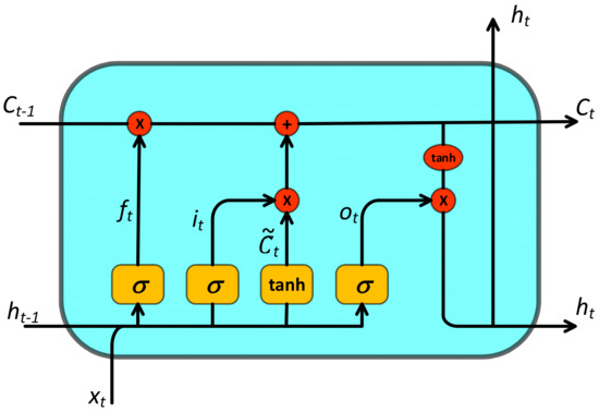
Figure 1.
LSTM structure.
2.2. Particle Swarm Algorithm
Indeed, the LSTM algorithm, known for its ability to retain information over time, proves highly effective in simulating and predicting variable load processes of coal-fired units, given their typical time series nature. However, like many neural network models, LSTM relies on several hyperparameters, including the number of neurons and hidden layers. These hyperparameters significantly influence the accuracy and performance of the algorithm. Therefore, careful selection and tuning of these hyperparameters are crucial for optimizing the LSTM model’s predictive capabilities and overall effectiveness in capturing the complex dynamics of variable load processes in coal-fired units.
In this study, the PSO algorithm is employed to discover the optimal hyperparameters for the LSTM neural network. The PSO algorithm is a widely used optimization technique renowned for its efficiency, simplicity, and low computational resource requirements [33].
In essence, the PSO algorithm treats each combination of hyperparameters as a particle within a global swarm. These particles traverse different directions and velocities during the iterative process. Over time, they converge towards both individual and global optimal positions. This iterative movement enables the PSO algorithm to find the optimal solution for the function being optimized, facilitating a comprehensive global search for optimization [34].
The specific process of the PSO algorithm is outlined as follows:
- (1)
- Initialize the parameters of the particle swarm:
- Set the particle swarm size N;Define the particle space dimension D;Determine the maximum number of iterations kmax;Specify the individual learning factor c1 and the population learning factor c2.
- (2)
- Initialize the position and velocity of each particle:
- Assign random initial positions within the search space for each particle;Initialize the velocity of each particle according to Equation (7).
- (3)
- Update the position and velocity of each particle iteratively:
- Calculate the fitness value for each particle based on its current position;Update the particle’s velocity and position using the individual and global best positions encountered so far, as well as the learning factors c1 and c2.
- (4)
- Repeat step (3) until convergence or the maximum number of iterations is reached:
- Evaluate the fitness of each particle at its updated position;Update the particle’s velocity and position accordingly;Update the global best position if necessary.
The velocity of the particles is shown in Equation (7):
where r1 and r2 are [0,1] random numbers used to increase the randomness of the search, and w is the inertia weight. The first term of the polynomial is the inertia part, which represents the continuation of the particle to the previous motion state; the second term of the polynomial is the cognitive part, which represents the speed and direction of the particle itself towards the local optimal direction; and the third term is the social part, which represents the sharing of information and co-operation among the particles and is the speed and direction of the particle’s motion towards the global direction. xid, vid, pid,best, pd,gbest are the position vector, velocity vector, individual optimal solution, and group optimal solution of the particle, respectively, and the specific structure is shown in Equations (8)–(11):
The equation governing the update of particle position is presented as Equation (12):
In other words, the particle position in the next step is obtained by adding the vector sum of the particle position from the previous step and the particle velocity from the next step.
The optimization of hyperparameters for LSTM long and short-term neural networks is illustrated in Figure 2.
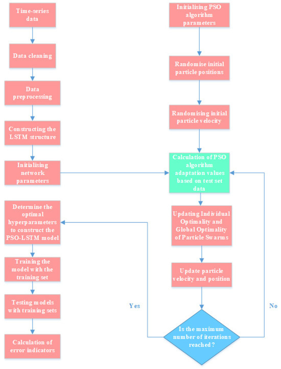
Figure 2.
Flowchart of hyperparameter optimization for LSTM long- and short-term neural networks.
3. Model Development
3.1. Data Preprocessing
The data utilized for the PSO-LSTM model originates from the DCS of a supercritical 2 × 600 MW unit located in North China. This dataset encompasses essential control parameters, including load commands and loads across all levels. Extracted from the unit’s monitoring and control information system, the second-level time series data spanning from May to July 2018 are employed for model training and testing, amounting to a total of 777,600 data points.
The dataset underwent scrutiny for missing values. Given that the load instructions and load data represent continuous time series, an interpolation approach was adopted to address missing values. Specifically, the average of the preceding and succeeding values at the missing positions was computed and used to fill in the gaps. Subsequently, the data were segregated into characteristic and target quantities [35].
The characteristic quantity ULD represents the specified value of unit load, as depicted in Equation (13):
The target quantity MW represents the output power of the generator, as shown in Equation (14):
In order to simulate the variable load response of the unit’s AGC, the input quantity comprises the feature quantity of the preceding two seconds, while the target quantity is shifted forward by two time steps. This adjustment ensures that the data required for model training maintain a one-to-one correspondence in terms of the time sequence. Any unmatched data at the end of the sequence are excluded. Additionally, the data are dimensionally restructured to facilitate sliding window input for the feature quantity. The input dataset is obtained from Equations (15) and (16).
The dataset is partitioned into training and test sets in an 8:2 ratio. Subsequently, both the training and test sets are normalized according to Equation (17), ensuring that the data conform to a normal distribution with a mean of 0 and a standard deviation of 1 [36].
where Dmean and Dstd are the mean and standard deviation of the data set.
3.2. Preliminary Model Calculations
The dataset is partitioned into a training set and a test set in an 8:2 ratio. Following the definition of the initial parameters of the LSTM neural network, the training set is fed into the model. The specific initial parameter configurations are presented in Table 1. With an increasing number of iterations, the mean square error of both the training and test sets gradually approaches zero. The test set is utilized for model validation to derive error metrics such as MAE, MAPE, RMSE, and R2, facilitating an initial assessment of the model. The error metrics are presented in Table 2. Comparison of predicted and actual output power is shown in Figure 3.

Table 1.
Model initial parameter settings.

Table 2.
Error between predicted and true values of the test set.
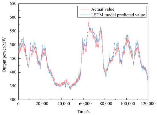
Figure 3.
Comparison of predicted and actual output power.
The comparison between predicted and actual values is depicted in Figure 3, illustrating that the initial AGC variable load digital model for thermal power units can to some extent forecast power generation during the variable load process. Nonetheless, in real-world scenarios, simulating longer control processes necessitates numerous model iterations, resulting in a gradual amplification of model errors. Hence, there remains potential for enhancing the accuracy of the digital model.
3.3. PSO Particle Swarm Algorithm to Optimize Numerical Models
The optimization of crucial hyperparameters in the model is conducted using the PSO algorithm [37]. The process begins by initializing the random particles’ initial position and velocity, followed by setting parameters such as the individual learning factor c1, population learning factor c2, and inertia weight w. These key hyperparameters for optimization are constrained within specific ranges, as detailed in Table 3 and Table 4.

Table 3.
PSO algorithm parameter settings.

Table 4.
Hyperparameter optimization range settings.
Once the model parameters are established, the PSO model is integrated with the thermal unit AGC variable load digital model, and the LSTM model’s hyperparameters are optimized using the PSO algorithm. The digital model undergoes several iterations of optimization as per Equation (7), and the variations in PSO adaptation value and LSTM hyperparameters during the calculation process are illustrated in Figure 4. The optimized parameters obtained from the optimization search are detailed in Table 5.
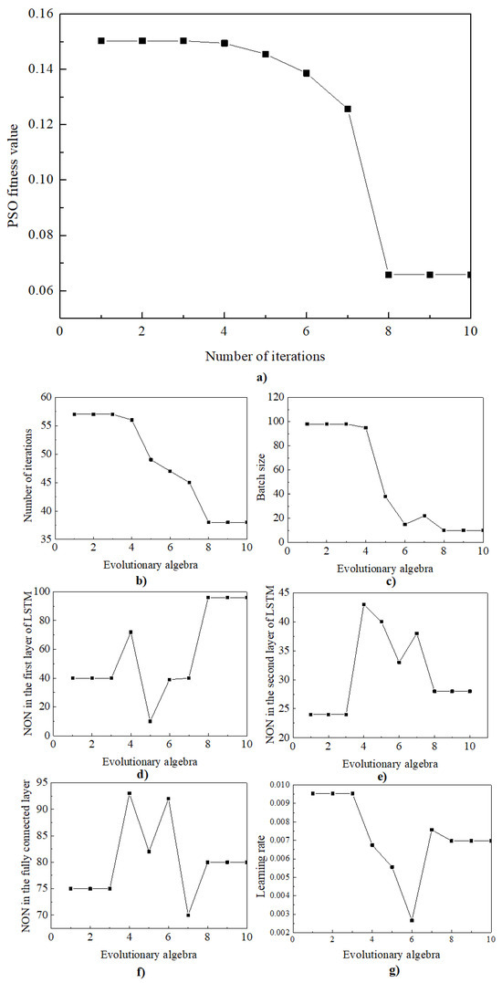
Figure 4.
PSO optimization iterative process.

Table 5.
Optimal hyperparameter settings.
The best parameters optimized using the PSO algorithm are utilized to update the hyperparameters of the LSTM long- and short-term neural network model. By inputting the same dataset into the updated model, the optimized numerical model’s performance on the test set is illustrated in Figure 5 and summarized in Table 6.
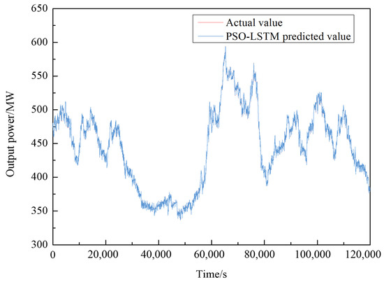
Figure 5.
Comparison of predicted and true values after PSO optimization.

Table 6.
Test set prediction and true value errors after the optimization process.
The application of the PSO algorithm notably enhances the model’s accuracy, leading to an improved fit between the predicted values and the actual values by 10.8%.
3.4. Model Validation
3.4.1. Dymola-Based Physical Modeling
As equipment aging and performance degradation are inevitable over years of operation, actual operational data may deviate from the design values. Therefore, in order to improve the credibility and applicability of this study in engineering applications and to provide more data, as well as controls for the data model, we chose the Dymola simulation software to simulate the unit. The digital model is then verified in two dimensions: through physical modeling calculation results and comparison with actual operational data. This software allows for the integration of physical relationships and control logic within the coal-fired unit, enabling dynamic simulation of thermal parameters and internal variables under near full load conditions using the Modelica simulation language. The specific unit chosen for simulation is a 600 MW supercritical power plant with primary intermediate reheat, a three-cylinder/four-extraction steam turbine, a single-axis configuration, and direct air-cooled condensing steam turbine technology. The boiler design is tailored for the coal type detailed in Table 7.

Table 7.
Coal type parameters for unit design.
The unit is modeled based on the specified design parameters outlined above. To simplify the modeling process, certain considerations are made as follows [38]:
- (1)
- The distinction between primary and secondary air is neglected, where the air necessary for coal combustion is preheated by the air preheater and introduced into the furnace.
- (2)
- Various losses such as air leakage losses on different sides (air, flue gas, and steam engine) and heat dissipation losses are disregarded.
- (3)
- Kinetic characteristics related to coal combustion are not accounted for.
- (4)
- The thermal system is assumed to have constant isentropic efficiency.
- (5)
- Mechanical inertia of the shaft is also overlooked.
Building upon this simplified model, a PID control system is integrated to regulate key system parameters, ensuring the stable operation of the model. The dynamic model, developed using Dymola software, is depicted in Figure 6.
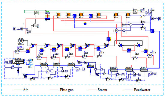
Figure 6.
Dynamic model of 600 MW supercritical direct air-cooled unit based on Dymola.
To validate the accuracy of the dynamic model simulation, the thermal parameters of the dynamic model under 100% THA condition are compared against the design parameters, and the specific errors are detailed in Table 8.

Table 8.
Validation of simulation results under 100% THA operating conditions.
The data presented in Table 8 demonstrate that the absolute value of the relative error between the dynamic model created with Dymola software and the designed steady-state data under 100% THA working condition does not exceed 0.2%. This level of accuracy is deemed sufficient to meet the practical requirements of the project.
3.4.2. Dymola-Based Numerical Model Validation
A segment of actual variable load process data from 20 September 2018 was chosen to test both the digital and physical models. The load command data were inputted into both the digital and physical models, and the resulting variable load dynamic curve is illustrated in Figure 7.
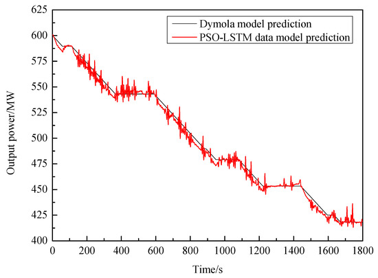
Figure 7.
Variable load dynamic curves of two models.
As depicted in Figure 7, upon comparing the actual values with the simulated values from both models, it is observed that both models can reasonably simulate the trend of the actual variable load process. The calculated goodness of fit R2 for the physical model is 0.954, while for the numerical model it is 0.998. Consequently, the numerical model can be deemed more accurate than the physical model in simulating the actual load instructions.
4. Results and Discussion
4.1. AGC Variable Load Process Study
To investigate the dynamic characteristics of the optimized numerical model’s AGC variable load process, simulations were conducted for load rising and load reduction processes from 75% THA to 100% THA using various load change rates. These simulations started from 0 s, and all load command changes followed primary function changes. The results of these simulations are presented in Figure 8 and summarized in Table 9.
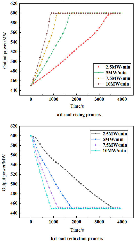
Figure 8.
Variation in output power at different variable load rates.

Table 9.
Overshooting at different variable load rates.
From the analysis of Figure 8 and Table 9, it is evident that the power generation response time during load raising process is slightly faster compared to load reduction. Moreover, as the load change rate in the model increases, there is a corresponding increase in the overshoot of actual generation power, and the intensity of fluctuations becomes more pronounced.
4.2. AGC Variable Operating Condition Evaluation Index
Due to the implementation of the “two regulations” in each regional grid of the power system, the demands on thermal power units have become increasingly stringent. Consequently, a more detailed and comprehensive evaluation index for AGC variable operating conditions in thermal power units has been developed [39]. A specific evaluation index for the “two regulations” is proposed [40], and its calculation method is outlined in Equations (18)–(20).
where K1 is the regulation rate index and K2 is the regulation accuracy index; λ1 and λ2 are the weighting coefficients, the sum of which is 1; Km is the measured AGC regulation rate of the unit, and Kb is the basic response rate of the unit; β is the precision deflation coefficient, which is used to unify the order of magnitude of the two indexes; P1(t) is the actual output of the unit under the process of variable load of the AGC, and P2(t) is the target output of the unit after the action of the AGC; and T is the time of input of the AGC.
4.3. Load Command Optimization
The load command input into the simulated AGC variable load process above is currently set using a basic primary function. To establish the optimal load command settings and refine the AGC variable load control process, the numerical model developed in this study can be applied to simulate the AGC variable load process. Initially, the load command settings are determined based on the relationship, as depicted in Equations (21) and (22), enabling the generation of various load command sets.
where U is the load command, T is the time, and γ is the power index, which is set to change the load command by setting different values; a and b are constants, which are determined by Equation (22) and the variable load process; c is the initial value of the load; and T1 is the time for the load command to reach the target load. The power function is chosen as a function to determine the relationship between load command and time, and the derivative of the load command is 0 when the target load is reached by Equation (22) in order to reduce the loss of economy and safety of the unit caused by the amount of overshoot of the AGC variable load.
As an example, considering a 50–75% THA variable load with a load change rate of 10 MW/min and T1 = 900 s, the load instruction changes are illustrated in Figure 8. Various load command sets are input into the deep learning model to derive P1(t), which is then used in conjunction with Equation (20) to compute the comprehensive evaluation index for variable load. In this calculation, the accuracy deflation factor b is set to 0.01, and λ1 = λ2 = 0.5. The variable load evaluation indexes under different load command settings are detailed in Table 10 and Table 11.

Table 10.
Comprehensive evaluation indexes of variable load under different load reduction commands.

Table 11.
Comprehensive evaluation indexes of variable load under different load rising commands.
The analysis presented in Table 10 and Table 11 reveals an inverse relationship between γ and stabilization time during both load rising and load reduction processes. This phenomenon arises due to the nature of γ: a larger value indicates a more abrupt initial change in the load command, followed by a smoother transition towards the final change. Consequently, while the load experiences greater variation at the onset, the system gradually adapts during subsequent periods, reducing the system’s instability during the response transition and hastening the time needed to attain a stable state.
However, it is essential to note that while within the experimental range a decrease in stabilization time is observed with increasing γ, such conclusions have limits. When γ becomes sufficiently large, the load command undergoes very sharp changes initially, potentially causing significant oscillations or overshoots in the system. This can lead to a longer recovery time and a delay in reaching the stable state, ultimately resulting in an increased stabilization time. Thus, the impact of γ on stabilization time exhibits a nuanced relationship that depends on the specific system dynamics and the extent of load command changes.
The regulation rate indicator K1 exhibits a decreasing trend with increasing γ, observed during both load rising and load reduction processes. This behavior can be attributed to the relationship between γ and the initial load command change. Specifically, as γ increases, the load command undergoes a more abrupt change at the beginning. Consequently, the output power also begins to change drastically earlier, leading to an earlier attainment of the target command. This early convergence towards the target load results in a decrease in the regulation rate indicator K1 as γ increases.
The regulation accuracy index K2 exhibits a non-linear trend with respect to γ in both the load rising and load reduction processes. Initially, K2 decreases as γ increases, indicating that when the load command changes steeply followed by a smooth transition, the control system may experience over-regulation or oscillations, leading to reduced regulation accuracy. Conversely, when the load command changes smoothly and then steeply, the system can adjust the load more gently, albeit potentially resulting in a slower regulation response and reduced timeliness in regulation accuracy. Therefore, an optimal value of γ is crucial to achieve the best regulation accuracy, striking a balance between rapid response to load changes and maintaining stability to ensure effective regulation.
In summary, the comprehensive evaluation indicator Ik demonstrates a non-linear trend with increasing γ. Specifically, within the experimental range, γ = 1.8 yields optimal comprehensive evaluation indicators for the regulation accuracy and regulation rate. However, it is important to note that this study offers a generalized approach and guidance for load command optimization in coal-fired power plants. The applicability of these conclusions may vary for other coal-fired power plants due to differences in load command strategies, control systems, and system configurations. Nonetheless, this methodology provides a framework for evaluation that can be adapted and applied across various coal-fired power plant contexts.
5. Conclusions
In this study, operational data from a 600 MW supercritical unit in North China was collected and processed to ensure its quality. We then employed an LSTM long short-term neural network to model the AGC variable load process of the unit. The model was rigorously tested using dedicated test set data and subsequently fine-tuned using the PSO algorithm for optimization purposes. Comprehensive validations of the data model were conducted using Dymola simulation software, revealing a high level of accuracy and effectiveness in simulating actual variable load conditions. Furthermore, comprehensive evaluation indexes were introduced and applied within the variable load process. These indexes were instrumental in evaluating the dynamic characteristics of coal-fired units under various load commands. By optimizing these load commands based on the evaluation indexes, we derived optimal settings that offer valuable guidance for the load command values during the peaking process of coal-fired units. The key conclusions drawn from this study are as follows:
- (1)
- The preliminary LSTM model was optimized using the PSO algorithm, which involved continuously updating the individual and population optima of particle positions. This optimization process led to a 10.8% improvement in the goodness of fit of the optimized model compared to the initial model.
- (2)
- The study utilized the data model to analyze the AGC variable load process, revealing several important findings. Specifically, it was observed that the generation power response rate during load rising process was slightly higher than during load reduction process. Additionally, faster load change rates in the model correlated with larger overshoots in actual generation power and more pronounced fluctuations.
- (3)
- Through numerical model simulations, an optimal variable load instruction set was determined within the experimental range. Notably, the load changing process demonstrated the smallest comprehensive evaluation index at γ = 1.8, representing the optimal load changing instruction set that balances safety and economy. The optimization of instructions based on the numerical model significantly improved the comprehensive system performance index by 55.1% for the load rising process and 54.2% for the load reduction process. These results highlight the numerical model’s ability to enhance the comprehensive performance of AGC’s variable load process while maintaining a high level of accuracy.
In this study, the PSO-LSTM data model is used to predict the output power under various load commands and determine the optimal value, which is a guide for the setting of load commands for coal-fired units, and the method can be used to calculate the output power before varying the loads for different operating conditions for different coal-fired units. However, there are some limitations of this study. For example, the analyses conducted using the data model are relatively superficial in terms of exploring the intrinsic mechanisms. In addition, the functions considered in the load command optimization process are relatively simple and beneficial to the operation of coal-fired units but lack in-depth theoretical analysis. It is hoped that these limitations will be further explored in future studies.
Author Contributions
Conceptualization, X.H.; Methodology, C.Y.; Software, H.C.; Validation, J.B.; Formal analysis, H.W.; Investigation, W.Z.; Writing—original draft, J.D.; Writing—review & editing, J.D. All authors have read and agreed to the published version of the manuscript.
Funding
This work was supported by the Science and Technology Project of the StateGrid Hebei Electric Power Co. (No. TSS2022-04).
Data Availability Statement
The original contributions presented in the study are included in the article, further inquiries can be directed to the corresponding authors.
Conflicts of Interest
Authors Xiaoguang Hao, Chunlai Yang, Jiandong Bao, Hui Wang and Wenbin Zhang were employed by the company State Grid Hebei Energy Technology Service Co., Ltd. The remaining authors declare that the research was conducted in the absence of any commercial or financial relationships that could be construed as a potential conflict of interest.
Nomenclature
| Superscripts and subscripts | |
| b | basic |
| m | measured |
| id | ideal |
| std | standard |
| Abbreviations | |
| AGC | Automatic Generation Control |
| DCS | Distributed Control System |
| GRU | Gate Recurrent Unit |
| MAPE | Mean Absolute Percentage Error |
| NON | Number of Output Neurons |
| PSO | Particle Swarm Optimization |
| RNN | Recurrent Neural Networks |
| BP | Back Propagation |
| GDP | Gross Domestic Product |
| MAE | Mean Absolute Error |
| MLP | Multilayer Perceptron |
| LSTM | Long Short-Term Memory |
| RMSE | Root Mean Square Error |
| THA | Turbine Heat Acceptance |
References
- Liu, J.; Lin, Y.; Jiang, M.; Guo, X. Exploring policy support for wind power development from a balancing perspective—A study of dynamic strategies based on evolutionary game. Energy Policy 2024, 188, 114061. [Google Scholar] [CrossRef]
- Raihan, A.; Mainul Bari, A.B.M. Energy-economy-environment nexus in China: The role of renewable energies toward carbon neutrality. Innov. Green Dev. 2024, 3, 100139. [Google Scholar] [CrossRef]
- Xie, Y.; Wu, X.; Hou, Z.; Li, Z.; Luo, J.; Lüddeke, C.T.; Huang, L.; Wu, L.; Liao, J. Gleaning insights from German energy transition and large-scale underground energy storage for China’s carbon neutrality. Int. J. Min. Sci. Technol. 2023, 33, 529–553. [Google Scholar] [CrossRef]
- Feng, T.-T.; Gong, X.-L.; Guo, Y.-H.; Yang, Y.-S.; Pan, B.-B.; Li, S.-P.; Dong, J. Electricity cooperation strategy between China and ASEAN countries under ‘The Belt and road’. Energy Strat. Rev. 2020, 30, 100512. [Google Scholar] [CrossRef]
- Obiora, S.C.; Olusola, B.; Hu, Y.; Ozsahin, D.U.; Adun, H. Assessing the decarbonization of electricity generation in major emitting countries by 2030 and 2050: Transition to a high share renewable energy mix. Heliyon 2024, 10, e28770. [Google Scholar] [CrossRef] [PubMed]
- Cao, J.; Ho, M.S.; Ma, R.; Zhang, Y. Transition from plan to market: Imperfect regulations in the electricity sector of China. J. Comp. Econ. 2024, 52, 509–533. [Google Scholar] [CrossRef]
- Ji, W.; Hong, F.; Zhao, Y.; Liang, L.; Du, H.; Hao, J.; Fang, F.; Liu, J. Applications of flywheel energy storage system on load frequency regulation combined with various power generations: A review. Renew. Energy 2024, 223, 119975. [Google Scholar] [CrossRef]
- Ju, L.; Lv, S.; Zhang, Z.; Li, G.; Gan, W.; Fang, J. Data-driven two-stage robust optimization dispatching model and benefit allocation strategy for a novel virtual power plant considering carbon-green certificate equivalence conversion mechanism. Appl. Energy 2024, 362, 122974. [Google Scholar] [CrossRef]
- Xu, Y.; Mu, Y.; Qi, H.; Li, H.; Yu, P.; Sun, S. Optimal dispatch approach for rural multi-energy supply systems considering virtual energy storage. Glob. Energy Interconnect. 2023, 6, 675–688. [Google Scholar] [CrossRef]
- Abouemara, K.; Shahbaz, M.; Mckay, G.; Al-Ansari, T. The review of power generation from integrated biomass gasification and solid oxide fuel cells: Current status and future directions. Fuel 2024, 360, 130511. [Google Scholar] [CrossRef]
- Zhou, S.; Bai, Z.; Li, Q.; Yuan, Y.; Wang, S. Potential of applying the thermochemical recuperation in combined cooling, heating and power generation: Optimized recuperation regulation with syngas storage. Appl. Energy 2024, 353, 122128. [Google Scholar] [CrossRef]
- Nik, A.; Karim, A. Shaping the Green Economy Through Application of Renewable Technologies and Industrialization. In Reference Module in Earth Systems and Environmental Sciences; Elsevier: Amsterdam, The Netherlands, 2024. [Google Scholar]
- Rana, M.; Uddin, M.; Sarkar, R.; Meraj, S.T.; Shafiullah, G.; Muyeen, S.; Islam, A.; Jamal, T. Applications of energy storage systems in power grids with and without renewable energy integration—A comprehensive review. J. Energy Storage 2023, 68, 107811. [Google Scholar] [CrossRef]
- Peng, W.; Chen, H.; Liu, J.; Zhao, X.; Xu, G. Techno-economic assessment of a conceptual waste-to-energy CHP system combining plasma gasification, SOFC, gas turbine and supercritical CO2 cycle. Energy Convers. Manag. 2021, 245, 114622. [Google Scholar] [CrossRef]
- Luo, Q.; Wang, W.; Fan, Q.-W.; Xu, C. Analysis of boiler dynamic response of thermal power unit with fast variable load. Therm. Power Eng. 2019, 34, 78–84. (In Chinese) [Google Scholar]
- Yong-liang, Z.; Bao-sheng, D.; Xiang, H. Simulation study on dynamic characteristics of variable load process of 660 MW supercritical coal-fired unit. China Electr. Power 2019, 52, 13–20. (In Chinese) [Google Scholar]
- Zlatkovikj, M.; Li, H.; Zaccaria, V.; Aslanidou, I. Development of feed-forward model predictive control for applications in biomass bubbling fluidized bed boilers. J. Process Control 2022, 115, 167–180. [Google Scholar] [CrossRef]
- Huang, C.; Li, Z.; Wang, Y.; Fang, F.; Liu, H.; Chen, Z.; Liu, Y. Influence of secondary air blade angle and oxygen-rich combustion characteristics of an improved Babcock swirl burner. Appl. Therm. Eng. 2024, 241, 122383. [Google Scholar] [CrossRef]
- Liu, G.; Liu, J.; Gao, P.; Yu, J.; Pu, Z. Understanding mechanisms of digital transformation in state-owned enterprises in China: An institutional perspective. Technol. Forecast. Soc. Chang. 2024, 202, 123288. [Google Scholar] [CrossRef]
- Irankhah, A.; Yaghmaee, M.H.; Ershadi-Nasab, S. Optimized short-term load forecasting in residential buildings based on deep learning methods for different time horizons. J. Build. Eng. 2024, 84, 108505. [Google Scholar] [CrossRef]
- Tian, Z.; Wang, Z.; Chong, D.; Wang, J.; Yan, J. Coordinated control strategy assessment of a virtual power plant based on electric public transportation. J. Energy Storage 2023, 59, 106380. [Google Scholar] [CrossRef]
- Si, R.C.; Wang, S.H.; Liu, X.W.; Li, J.; Zhou, C.; Li, B.J. Power unit load system modelling research based on BP neural network. In Proceedings of the 4th International Conference on Energy Engineering and Environmental Protection (EEEP), Sanya, China, 19–21 November 2019. [Google Scholar]
- Zhang, G.; Zhang, C.; Wang, W.; Cao, H.; Chen, Z.; Niu, Y. Offline reinforcement learning control for electricity and heat coordination in a supercritical CHP unit. Energy 2023, 266, 126485. [Google Scholar] [CrossRef]
- Wang, Z.; Liu, M.; Yan, H.; Zhao, Y.; Yan, J. Improving flexibility of thermal power plant through control strategy optimization based on orderly utilization of energy storage. Appl. Therm. Eng. 2024, 240, 122231. [Google Scholar] [CrossRef]
- Li, G.; Du, G.; Liu, G.; Yan, J. Study on the dynamic characteristics, control strategies and load variation rates of the concentrated solar power plant. Appl. Energy 2024, 357, 122538. [Google Scholar] [CrossRef]
- Wang, X.; Cui, C.; Pan, C.; Zhang, C.; Ren, H.; Ghias, A.M. A deep reinforcement learning control strategy to improve the operating flexibility of CHP units under variable load conditions. Therm. Sci. Eng. Prog. 2024, 49, 102482. [Google Scholar] [CrossRef]
- Jung, Y.G.; Lee, K.H.; Park, B.R.; Kim, T.W.; Moon, J.W. Development and performance evaluation of intelligent algorithm for optimal control of a hybrid heat pump system during the cooling season. Energy Build. 2024, 306, 113934. [Google Scholar] [CrossRef]
- Mate, S.; Pal, P.; Jaiswal, A.; Bhartiya, S. Simultaneous tuning of multiple PID controllers for multivariable systems using deep reinforcement learning. Digit. Chem. Eng. 2023, 9, 100131. [Google Scholar] [CrossRef]
- Elman, J.L. Distributed Representations, Simple Recurrent Networks, and Grammatical Structure. Mach. Learn. 1991, 7, 195–225. [Google Scholar] [CrossRef]
- Bengio, Y.; Simard, P.; Frasconi, P. Learning long-term dependencies with gradient descent is difficult. IEEE Trans. Neural Netw. 1994, 5, 157–166. [Google Scholar] [CrossRef] [PubMed]
- Hochreiter, S.; Schmidhuber, J. Long Short-Term Memory. Neural Comput. 1997, 9, 1735–1780. [Google Scholar] [CrossRef]
- Graves, A.; Mohamed, A.R.; Hinton, G. Speech recognition with deep recurrent neural networks. In Proceedings of the 2013 IEEE International Conference on Acoustics, Speech, and Signal Processing (ICASSP), Vancouver, BC, Canada, 26–31 May 2013; pp. 6645–6649. [Google Scholar]
- Ahmad, A.; Yadav, A.K. Parametric analysis of wastewater electrolysis for green hydrogen production: A combined RSM, genetic algorithm, and particle swarm optimization approach. Int. J. Hydrog. Energy 2024, 59, 51–62. [Google Scholar] [CrossRef]
- Zhang, X. Design optimization of irregularity RC structure based on ANN-PSO. Heliyon 2024, 10, e27179. [Google Scholar] [CrossRef] [PubMed]
- Mondal, R. Micro-segregated two-dimensional fluid and mass transport modelling in unsteady rotating annular photocatalytic reactor. Results Eng. 2022, 16, 100752. [Google Scholar] [CrossRef]
- Li, Y.; Li, Z.; Wang, H.; Cai, N. CaO carbonation kinetics determined using micro-fluidized bed thermogravimetric analysis. Fuel 2020, 264, 116823. [Google Scholar] [CrossRef]
- Liang, X.; Li, W.; Zhang, Y.; Zhong, Y.; Zhou, M. Recent advances in particle swarm optimization via population structuring and individual behavior control. In Proceedings of the Networking, Sensing and Control (ICNSC), 2013 10th IEEE International Conference, Evry, France, 10–12 April 2013. [Google Scholar]
- Yang, C.; Hao, X.; Zhang, Q.; Chen, H.; Yin, Z.; Jin, F. Performance Analysis of a 300 MW Coal-Fired Power Unit during the Transient Processes for Peak Shaving. Energies 2023, 16, 3727. [Google Scholar] [CrossRef]
- Feng, D.; Zhao, Y.; Su, H.; Li, H.; Zhou, Y. Bi-level decomposition algorithm of real-time AGC command for large-scale electric vehicles in frequency regulation. J. Energy Storage 2023, 62, 106852. [Google Scholar] [CrossRef]
- Wang, Y.; Wang, K. Load control system performance evaluation method considering “two rules”. J. Syst. Simul. 2021, 33, 710–720. (In Chinese) [Google Scholar]
Disclaimer/Publisher’s Note: The statements, opinions and data contained in all publications are solely those of the individual author(s) and contributor(s) and not of MDPI and/or the editor(s). MDPI and/or the editor(s) disclaim responsibility for any injury to people or property resulting from any ideas, methods, instructions or products referred to in the content. |
© 2024 by the authors. Licensee MDPI, Basel, Switzerland. This article is an open access article distributed under the terms and conditions of the Creative Commons Attribution (CC BY) license (https://creativecommons.org/licenses/by/4.0/).