Abstract
In the increasingly complex and dynamic electrical power system, forecasting harmonics is key to developing and ensuring a clean power supply. The traditional methods have achieved some degree of success. However, they often fail to forecast complex and dynamic harmonics, highlighting the serious need to improve the forecasting performance. Precise forecasting of electrical power system harmonics is challenging and demanding, owing to the increased frequency with harmonic noise. The occurrence of harmonics is stochastic in nature; it has taken a long time for the development of dependable and efficient models. Several machine learning and statistical methods have produced positive results with minimal errors. To improve the prognostic accuracy of the power supply system, this study proposes an organic hybrid combination of a convolutional neural network (CNN) and bidirectional long short-term memory (BiLSTM) with the attention mechanism (AM) method (CNN-BiLSTM-AM) to forecast load harmonics. CNN models intricate non-linear systems with multi-dimensionality aspects. LSTM performs better when dealing with exploding gradients in time series data. Bi-LSTM has two LSTM layers: one layer processes data in the onward direction and the other in the regressive direction. Bi-LSTM uses both preceding and subsequent data, and as a result, it has better performance compared to RNN and LSTM. AM’s purpose is to make desired features outstanding. The CNN-BiLSTM-AM method performed better than the other five methods, with a prediction accuracy of 92.366% and a root mean square error (RMSE) of 0.000000222.
1. Introduction
The wide usage of variable speed drives (VSDs), rectifiers, and inverters creates non-linear loads in a power network, resulting in non-sinusoidal current that is non-linearly related to the supply voltage. The non-sinusoidal current is a periodic function, and it can be decomposed into its fundamental sine wave plus various other sine waves of harmonic frequencies. Harmonics are an integral of multiples of the fundamental frequency. Thus, a non-sinusoidal current may have both odd and even harmonics. Harmonics have a negative impact on the reliability, stability, and safety of a power network. They may cause power supply interruptions, abnormal grounding protection, shorten equipment life, and overheat conductors as well as equipment [1]. This, in turn, has a cascading impact on equipment downtime, ultimately diminishing the overall system productivity. Identifying abnormal behavior in equipment is gaining recognition as a pivotal element in proactively anticipating necessary maintenance actions [1]. Both current and voltage harmonics are non-linear, non-stationary, dynamic, complex, noisy, and unstable and are classified as time series. These characteristics make harmonics difficult to predict.
Figure 1 shows a typical Nestle plant VSD connection of two electric motors. Most of the three-phase VSDs employ six-pulse-bridge “uncontrollable” diode rectifiers or “half-controllable” silicon-controlled rectifiers (SCRs) that are used to convert AC power to DC power that is used by variable frequency converters (VFCs). These circuits are low in cost, simple, and highly reliable. However, the conversion process produces significant harmonic currents that trigger system resonance at (Figure 1), which causes relatively high-voltage harmonics across the point of common coupling (PCC). All these phenomena pollute the power supply, leading to poor power quality. LC passive filters (de-tuned filter banks and fine-tuned filters) are used to address harmonics issues. Other measures include active filtering, inductive reactance, and high-pulse rectifiers. Nevertheless, filters are not quite cost-effective for dealing with these issues. In some instances, differential mode (DM) and common ode (CM) noise like electromagnetic interference (EM) filters are added to the filter circuit (Figure 1), but this increases the risk of resonance in a multi-drive system, like the one at the Nestle Chocolate factory in East London, Eastern Cape Province of South Africa.
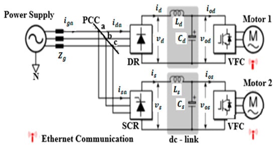
Figure 1.
A typical plant VSD connection.
Machine learning (ML) techniques model complex and non-linear problems better than statistical techniques. The precise detection of harmonics is critical to an electrical power network’s efficiency and reliability. Harmonics degrade the quality of an electrical power supply by causing steady-state waveform distortion [2]. An effective harmonics prediction method is a useful tool in planning an efficient electrical power network. Power network efficiency is characterized by its reliability and system reliability and is a function of cost-saving. The widespread use of electronic converters and inverters contributes to distorting both the voltage and current waveforms, resulting in harmonics. Statistical and machine learning algorithms have been used in forecasting power consumption, fault prediction on machines, and the number of time series data, but work is still being performed to find more accurate algorithms for the prediction of harmonics in an electrical power network [3,4,5,6,7].
To the best of our knowledge, the application of CNN-BiLSTM-AM has not been extensively utilized in the prediction of electrical load harmonics, marking this research as pioneering in this specific field. This work is built on our previous work on the application of ANN, LSTM, and CNN-LSTM in the detection and prediction of harmonics in an electrical power system [8,9,10]. In this paper, six (6) models are used to predict the load harmonics and are separately trained and tested using the historical harmonics data. The independent results are analyzed to determine the most accurate model, and RMSE is the method performance indicator. The paper’s contribution is to (1) propose an innovative method of harmonics detection and prediction based on a hybrid CNN-BiLSTM-AM model; (2) compare CNN-BiLSTM-AM model harmonics forecasting capabilities with five other deep learning methods; and (3) demonstrate that the CNN-BiLSTM-AM network performed better than the other five models in detecting and forecasting of harmonics. The paper outline is as follows: Section 2 covers related work performed so far. Section 3 outlines the methodology used in this paper. The results are discussed in Section 4 and the conclusion in Section 5.
2. Review of Harmonics Forecasting
The literature review effectively contextualized the investigation by considering aspects such as scope and relevance, the identification of research gaps, rationale for the investigation, integration with investigation objectives, critical analysis, and synthesis, as well as scope limitations. This comprehensive approach ensured that the investigation’s context was well established, relevant research gaps were clearly identified, and the rationale for addressing these gaps was justified based on the existing literature. Additionally, the review critically analyzed prior research and synthesized diverse perspectives, providing a solid foundation for the current investigation’s contributions.
Fast Fourier transforms (FFTs), the zero-crossing method, the least squared method (LSM), the Prony method, and the Time-Domain Quasi-Synchronous Sampling method have traditionally been used in harmonics measurements [5]. These methods are challenged when they are used to manipulate big data. FFT has problems associated with spectrum leakage and picket fencing resulting from nonsynchronous sampling. These challenges are handled better using LSM based on the interpolation method, resulting in improved accuracy [6]. Most of these methods extract features in the time and frequency domains, and the associated challenges include the following: 1. Harmonics and many other power quality disturbances have almost similar features; this leads to poor feature selection. 2. Features captured in the time and frequency domains do not describe harmonic pollution, thus leading to poor selection accuracy. 3. A feature extraction process demands a high-level understanding of harmonics characteristics, leading to complex feature extraction [7].
Time series prediction techniques fall into two categories, namely, traditional time series methods and forecasting methods based on machine learning. Traditional time series techniques deal with specific models to describe time series, and they have challenges in dealing with real-world time series data due to their non-linearities [8]. The dynamic equation for time series is either complex or unknown, and as such, noisy and complex features would not be determined using analytical equations. These ML techniques require low-end hardware [9]. ML and DL methods are used to enhance network management, and these methods are bioinspired mathematical [10]. Support vector machines (SVMs), Random Forest, ARIMA, decision trees, and logistic regression are the most frequently used ML time series data approaches, and they tend to work better on small-scale data [11].
DL (deep learning), a branch of ML, is a data-driven methodology with the capability to handle prediction issues related to big data. On the other hand, signal processing techniques struggle with prediction issues related to big data. DL methods perform better when used to solve power quality disturbance challenges [12]. The DL method has shown good performance when dealing with high-dimension data, non-stationary data, and non-linear time series data [10]. The most popular deep learning (DL) methods are recurrent neural networks (RNNs), LSTM, BiLSTM, and CNN. These algorithms have densely connected neurons, resulting in high learning and generalization capabilities [13]. A ‘deep recurrent neural network with long short-term memory (DRNN-LSTM)’ was used to predict solar panel output including the load an hour ahead [14].
A deep neural network (DNN) is a developed and advanced artificial neural network (ANN) that is sequence-based and has the capability of learning and extracting features from inputs in the time series domain. RNN is a recurring neural network and has a unique network architecture, as shown in Figure 2. to represent the input variables, while to represent the output variables. A variable is a symbolic representation that can assume various values, categorized based on characteristics and context into types like independent, dependent, discrete, continuous, and categorical.
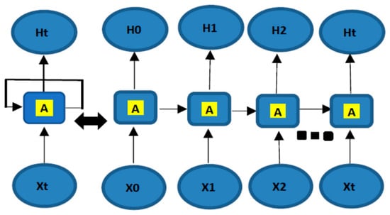
Figure 2.
RNN structure.
The output of the neuron is an input to the same neuron at the following time point, so that the output of the system at this instant comes from the interaction between the input of a particular time instant and all the time instances in memory. Consequently, it essentially lets signals move forwards and in reverse. In the time domain, the regression procedure has produced good results during wind speed forecast and current control [15]. RNN methods are many inputs to one output, many inputs to many outputs, and one input to many outputs. RNN is challenged when dealing with long-term dependencies that lead to vanishing gradients. LSTM is a specialized RNN capable of dealing with these long-term dependency challenges and has shown significant performance when dealing with time series data and forecasting [16]. RNN and particularly LSTM have been used in feature sequence extraction, for example, in transient periods, as well as data classification in power applications, including fault diagnosis of photovoltaic, wind turbines with multivariate time series, transmission lines, and the prediction of fault location distance in a two-bus line test system of 220 km [17]. There is no need to make assumptions when using LSTM, and it can deal with dynamic, non-linear, complex, and noisy data in a higher-dimensional space. The LSTM network transmits in the forward direction, and Bi-LSTM has a minimum of two LSTM layers arranged so that one LSTM layer processes data in the onward direction and the second LSTM layer in the reverse direction. This arrangement improves forecasting precision [18].
CNN is extensively used in the field of image processing and is steadily being used to predict time series data [19]. CNN has been applied in various electrical power systems relating to prediction and classification problems varying from harmonics, transients, islanding, instability, etc. CNN automatically extracts system features and is easy to train compared to other neural networks that have several hidden layers. CNN can also be used for 1-D inputs, like most power systems problems, and relies mainly on the convolutional and dense layers rendering the pooling layer less significant. It has been successfully used in a number of power system-related classification and prediction problems [20]. Figure 3 is the example of CNN 1-D architecture.
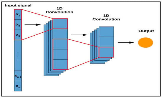
Figure 3.
CNN 1-D architecture [20].
CNN is combined with AM to focus on specific features, leaving unnecessary features and boosting the desired information. This enhances the feature selectivity of the chosen model [21]. CNN-BiLSTM with attention mechanism (AM) has been successfully used to identify a two-phase flow pattern in a multivariate time series. AM was used to select the highest values of the small vectors, as the vital features of the small vectors could not be detected and selected by CNN-BiLSTM layers. These vectors would be combined in the n-dimensional vector to give a vector of each medium-sized vector [22]. Hybrid LSTM with the AM model has been used in residential load forecasting and showed impressive results. AM is well suited for demand-side forecasting methods involving LSTM. LSTM cannot pick up inner correlations among the hidden features that have a significant impact on the forecast results. Thus, AM is deployed to mitigate this weakness by adaptively weighting the hidden features [23].
3. Methodology
The idea of DL was developed from the study of artificial neural networks (ANNs), a shallower learning algorithm. DL has multi-hidden layers and can perform a layer-by-layer transformation of data features, thereby extracting the most effective information from the data. DL is a data-driven algorithm, and it does not need to construct a physical model. It only needs historical data to extract optimal features of the power network and subsequently perform tasks such as harmonics/fault diagnosis, harmonics/fault classification, and prediction.
The aim is to build a DL machine model that can forecast the production of harmonics, thereby reducing the risk of machine breakdown. Supervised learning typically requires iterations of building and evaluating different models. Figure 4 shows the proposed model flowchart. The data are initially split into training and validation data. The model root mean square error (RMSE) loss is checked whether it is stable. If the RMSE error rate is not stable, the model will retrain; otherwise, the model will be validated, and the training ends. Once the model is trained, its performance is typically evaluated by comparing model predictions with known responses.
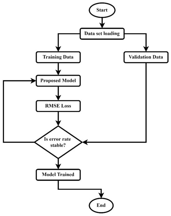
Figure 4.
Proposed model flowchart.
3.1. Data Analysis and Problem Formulation
The study is conducted using historical data collected at Nestle East London, South Africa. The dataset consisted of 8967 records between 06 January 2021 and 06 November 2021 (eleven months). It is very important to note that the data period is long, and harmonics data were reported hourly, but there were some periods within this interval where the data were not recorded for various reasons. Hence, to generate robust and reliable results, pre-processing was performed, and the null data were filtered out and removed. The data were smoothed out, and the cleaned raw data are shown in Figure 5a–e.
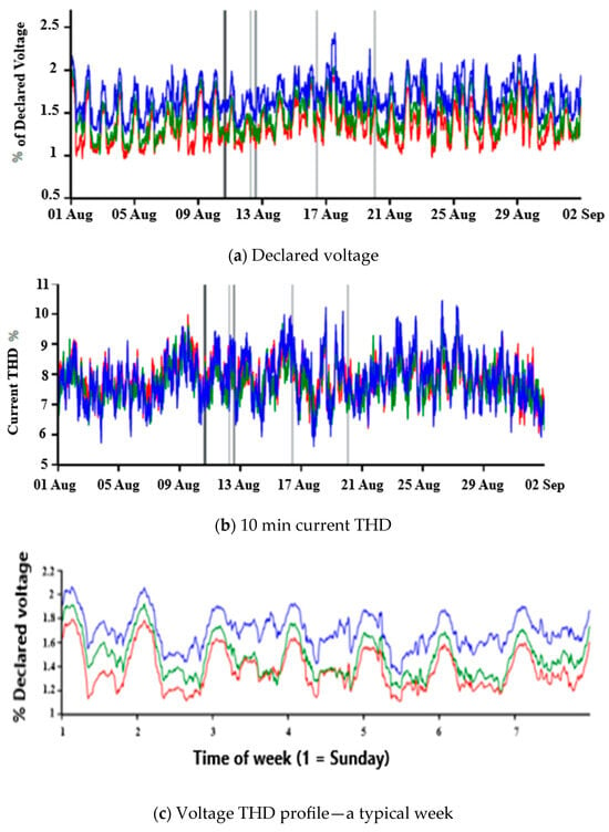
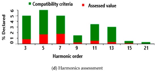
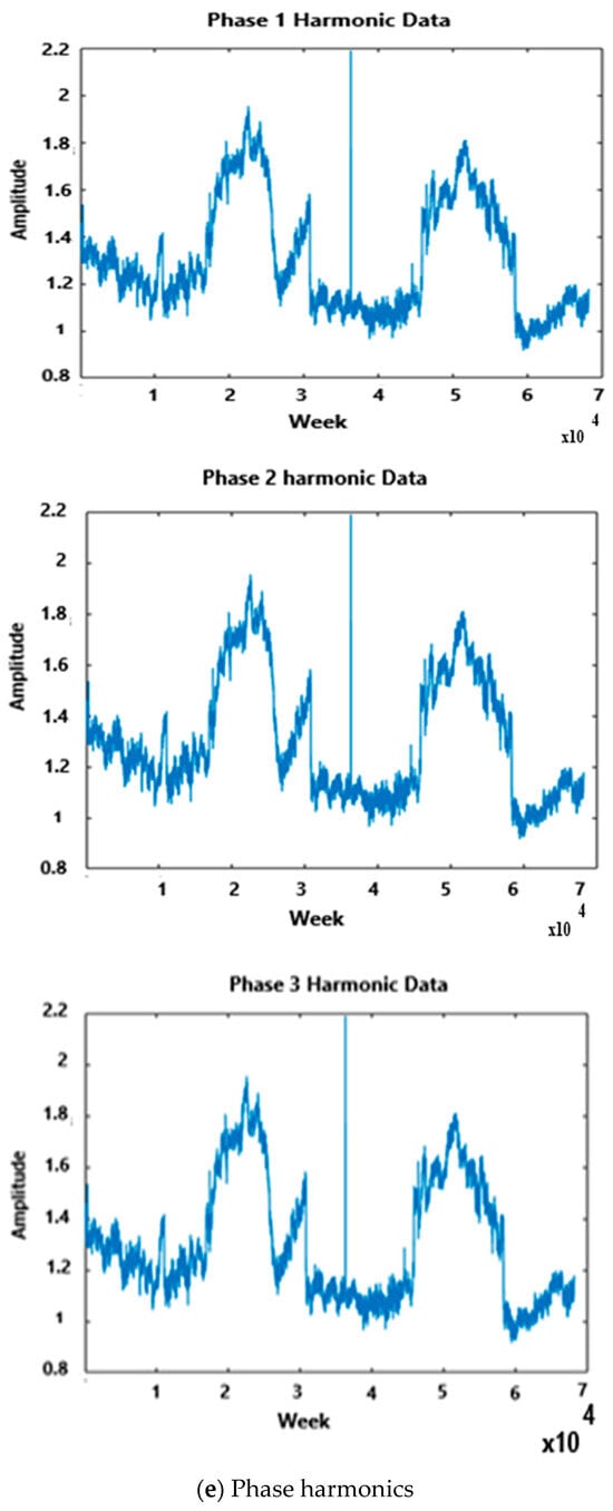
Figure 5.
(a–e): Measured harmonics.
The factory uses both variable frequency drives (VFDs) and variable speed drives (VSDs) for the speed control of DC and AC motors and variable source inverters (VSI) in uninterruptible power supplies (UPS) units. Modern VSDs use pulse-width modulation voltage source inverters (PWM VSIs) to control the speed of three-phase induction motors. The advantages of PWD VSI are extremely good dynamics, peak current protection, instantaneous current waveform control, better accuracy, compensation of load parameter changes effect, semiconductor voltage drop compensation, and dc link and ac side voltage changes compensation. VSDs and VFDs have numerous advantages, including the following: matching motor and load characteristics; energy-saving speed; and position control; the reduction of stresses as well as transients caused by ON/OFF; and sudden motion operations. VSDs may significantly decrease the quality of the alternating current (AC) to which they are connected, and they draw non-sinusoidal current from the main power AC supply, thus leading to the generation of high-order harmonics in the power supply. These harmonics are reduced by direct current (DC) chokes to maintain levels below the International Electro-technical Commission (IEC) 62,635 maximum standard measured total harmonics distortion (THD) index. The sample THD data that was used in this paper are shown in Figure 5a–e. The declared voltage represented a sample of the supply voltage, alongside current total harmonic distortion (THD), a typical three-phase voltage THD profile for a typical week measured at the plant, harmonic order data of the measured harmonics at the plant, and phase harmonic information. Figure 5e depicted the simulation results of harmonic data in MATLAB, aiming to gauge how closely the simulation aligned with the actual harmonics measured at the plant. The objective is to accurately manage the active filter’s reaction time delays and response using the proposed DL method. The filters are designed and used by manufacturing factories with non-linear and stochastic loads, like Nestle in East London. The Nestle confectionery plant emerged as one of the top five contributors to harmonics in the Buffalo City Municipality electrical distribution network. Nestle proactively supplied the requisite data, whereas the other four plants declined participation without clarification. The study specifically delved into utilizing AI techniques to forecast harmonics within the load-side subsystem of the electrical power system, mirroring earlier research that explored AI techniques for predicting harmonics in the generation and transmission subsystems.
The cleaning functions in MATLAB (illmissing, ismissing, rmmissing, filloutliers, rmoutliers, smoothdata, movmean, and movmedian) were used to enhance dataset quality. They filled in missing values, identified missing data, removed outliers, and reduced noise, ensuring data reliability for analysis and modeling.
3.2. Deep Learning Algorithms
3.2.1. Bi-Directional LSTM
BiLSTM architecture is best explained using the LSTM architecture as the fundamental building block. LSTM was developed to improve RNN weaknesses in dealing with long-term dependencies. The RNN model structure has a return loop that uses prior information efficiently. However, the RNN model has limited memory and does not learn long-term dependencies well, resulting in a vanishing gradient. The vanishing gradient phenomenon is when the input information or the gradient passes through several layers, then vanishes and washes out when it reaches the end. Consequently, RNN struggles to capture long-term dependencies and makes training much harder since the training algorithm assigns smaller values to the weights. When this happens, the RNN algorithm stops learning. Another challenge associated with this phenomenon is “exploding gradients”. Exploding gradients refer to situations where the input information or gradient passes through multiple layers, and by the time it reaches the end, the gradient is exceptionally large, making the training of RNN challenging. This challenge makes the training algorithm assign bigger values to the weights. In mitigation, the gradient can be truncated. The gradient is mathematically expressed as a partial derivative of the output of a function with respect to its input. Thus, the gradient determines how much the output changes with respect to the changes affecting the input. A Gated Recurrent Unit (GRU) shown in Figure 6 is used to mitigate the RNN gradient problems.
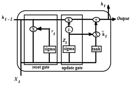
Figure 6.
GRU structure.
The input is ; the reset gate is ; , is hidden layer state output at the current and previous time; the update gate is ; tanh is an activation function; is a sigmoid function; and is the active state of a hidden layer at the present time. The GRU has been used in a hybrid model with AM in order to improve its performance [24]. GRU, short for “Gated Recurrent Unit,” represents a form of recurrent neural network (RNN) architecture. It serves as a modification of conventional RNNs and aims to tackle the challenge of the vanishing gradient problem encountered during the training of RNNs on lengthy sequences. GRUs integrate gating mechanisms that manage the information flow within the network, enhancing its capacity to comprehend dependencies across extended sequences. They find extensive application in natural language processing endeavors such as machine translation, text generation, and sentiment analysis, alongside various sequential data tasks like time series forecasting and speech recognition.
LSTM was developed based on GRU and was developed to deal with RNN limitations [25]. The LSTM model has memory cells that are used to remember long-term historical data, and Figure 7 shows the LSTM cell architecture. The data in an LSTM cell are regulated through three gate mechanisms, namely, the input gate , the forget gate , and the output gate . The input gate deals with the latest information that is fed into a cell by choosing which current information is maintained from the previous state; the forget gate regulates how much information must leave a cell and the output gate deals with how much information can leave the cell to the output. Memory plays a significant role in LSTM by enabling the network to selectively store and retrieve information over time. The start of the memory cell is performed through point-wise multiplication and sigmoid function operations. The input information at the current state, together with , forms the hidden state of the previous LSTM cell/layer and is fed into all the gates and transitioned by the sigmoid and tanh functions. A linear combination of the prior cell state and the current input is manipulated to update the cell when the gating mechanism is activated. The forget gate determines data that must be kept or rejected, and its output is anywhere between zero and one. If the forget output is leaning towards zero, then it means the information has been ignored, and if the information is close to one, then the data have been kept.
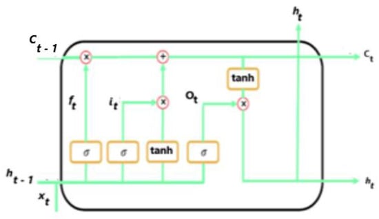
Figure 7.
LSTM cell architecture.
The forget operation is expressed mathematically as
where is the sigmoid activation function, is the weight, and is the bias. The vectorial summation of and is fed into all gates through the sigmoid and tanh activation functions. The input gate decides which data to update. The input gate is expressed as
The next step is to feed the current input state and the hidden state into the tanh function. At this stage, the cell state is determined, and the resulting value updates the cell state and is expressed by the equation.
where tanh is the activation function. A new memory state and new hidden state is passed on to the next state. is determined by the equation.
A single LSTM layer manipulates data in the forward direction. Bi-LSTM has two LSTM layers: one layer processes data in the onward direction and the other layer in the regressive direction, as shown in Figure 8. The LSTM layer in the forward direction receives the input past data information, and the reverse LSTM layer obtains the input sequences’ future information. Then, the output in both hidden layers is combined. The hidden state of Bi-LSTM at time t has forward and reverse and is expressed by the equation.
where is a summation of the forward and reverse components. Bi-LSTM uses both preceding and subsequent data, and as a result, it has better performance compared to RNN and LSTM.
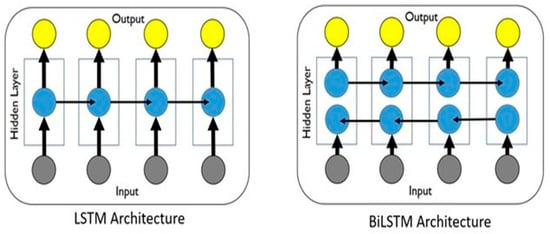
Figure 8.
LSTM and Bi-LSTM architecture.
3.2.2. Convolutional Neural Network
CNN, a deep learning method, is principally employed in image identification as well as progressively and steadily being utilized in time series data forecasts [11]. It models intricate non-linear systems with multi-dimensionality aspects. For example, given I (an image), a 2D convolution manipulation is expressed by the following:
where (i, j) is the pixel coordinate vector, I (i + u, j + v) is the image intensity at (i + u, j + v), W is weight, and b is bias. W and b are learned during the training phase. represents the convolution kernel feature at position (i, j), and k is the number of convolution kernels. During the training phase, the input layers are updated with the back propagation learning process, which results in an internal covariant transformation. Batch normalization is used to mitigate this problem. A non-linear down-sampling process, maximum pooling, is used to decrease the data dimension while at the same time retaining the invariability of image translation, expansion, and rotation [26].
Figure 9 shows the CNN architecture, consisting of stacking up the convolutional, pooling, and fully connected layers. The convolution layer has filters to extract features from the input pattern. The filters perform convolution processes through weight sharing and thus reduce the intricacy of the computational operations and increase the network performance [27]. The down-sampling process, used to reduce the dimensions of the features and overfitting, is performed by the pooling layer. The fully connected layer is used to learn the non-linear combinations of features and produces the output [28]. The CNN method has issues in learning relationships between time series data. A combination of RNN and CNN is used to mitigate this challenge.

Figure 9.
CNN structure.
3.2.3. Attention Mechanism
The purpose of the attention mechanism is to upgrade and make desired features outstanding, and it is motivated by the human visual system. When the human visual system observes a scene, it focuses on detail as needed. Thus, it does not observe the whole scene from start to finish. Therefore, AM selectively focuses on important feature information, ignores unnecessary feature information, and enhances the desired feature information. AM is used in image captioning and is increasingly applied to other fields, including time series data, like in this research. The AM process is illustrated in Figure 10.
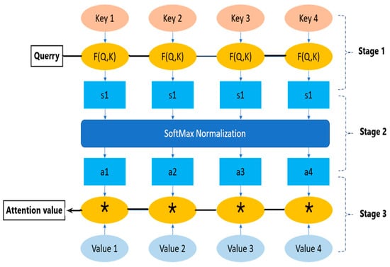
Figure 10.
Attention mechanism process.
The AM process is based on weight allocation, determining key and valuable information through the distribution of higher weights. It has three stages and is usually used after the CNN and Bi-LSTM networks to place emphasis on characteristics that contribute to the desired output and model performance improvement. The attention function is a mapping from a query to a sequence of key values. The similarity between the query and each key is calculated in the first stage using the mathematical expression.
where is the attention score, is the weight, is the input vector, and is the bias. The score obtained in stage one is normalized, and SoftMax function is employed to convert the attention score using the mathematical expression at stage two.
The final attention score is computed at stage 3 using the mathematical expression.
A SoftMax activation function is used for multi-class classification issues and is used as a last activation function of a neural network to normalize the output of the network to a probability distribution over the predicted output. It takes an input vector and produces a probability distribution over the classes at the output. Each element present in the output vector represents the probability of the input belonging to the class and the formula is as follows:
where x_i is the i-th element of the input vector, n is the size of the input vector, and is the exponential of the i-th element of the input, and the sum of it is over all elements j in the input vector. The SoftMax function has a feature that the sum of the output probabilities is equal to one and expressed by Equation (13).

This is of vital importance for tasks where the input can only belong to one of the several mutually exclusive classes. The SoftMax function is used in backpropagation algorithms since the function is differentiable.
3.2.4. CNN-Bi-LSTM Attention Model
CNN and Bi-LSTM networks are employed to fully extract the spatial and temporal features of the harmonics, and AM is used to focus on the characteristics that have a strong correlation with harmonics, making the prediction performance better. Firstly, the harmonics data are pre-processed. Secondly, the CNN is used to capture the spatial dependencies on the harmonics to reduce the dimension of the harmonics data so that effective spatial information is used. Thirdly, the temporal dependencies are captured using Bi-LSTM. Fourthly, the AM is used to highlight important harmonics features to achieve satisfactory prediction performance. Bi-LSTM has a good forecasting accuracy that would capture future and past harmonics data simultaneously. A reverse relationship of the data is considered to forecast the long-term and short-term production of stochastic harmonics efficiently. Figure 11 shows the model flowchart and layout. The input vectors are fed into the CNN layer, and the output is the input to the BiLSTM connected to the attention mechanism that is finally connected to the output.
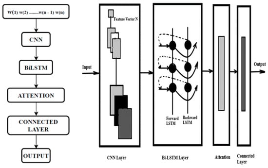
Figure 11.
CNN-Bi-LSTM attention model flowchart and layout.
The CNN-BiLSTM-AM architecture in Figure 11 comprises an input layer for receiving data, typically word embeddings or textual representations, followed by a convolutional neural network (CNN) to extract local features. These features are then passed to a bidirectional long short-term memory (BiLSTM) layer, which captures both past and future context to understand the sequential data comprehensively. An attention mechanism further refines the model’s focus by assigning weights to different parts of the input sequence, enhancing its ability to discern relevant information. Finally, the output layer generates the desired classification or regression output based on the specific task at hand. This architecture amalgamates the strengths of CNNs, BiLSTMs, and attention mechanisms, making it a potent choice for various natural language processing tasks. Given the dataset’s considerable size, the experimentation utilized a Core i7 processor and started with 3 million epochs and continues to increase the number of epochs to 4.5 million, which gave better results, as shown in Figure 12. Figure 12a show the final results while Figure 12b shows progress results.
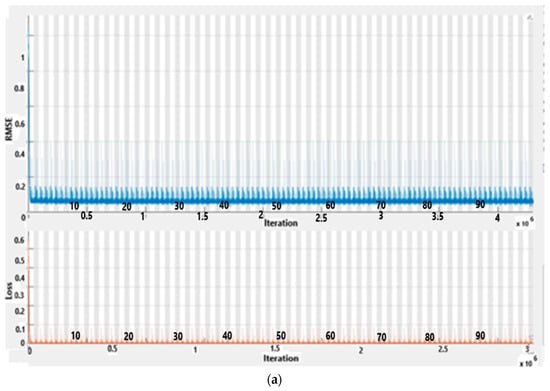
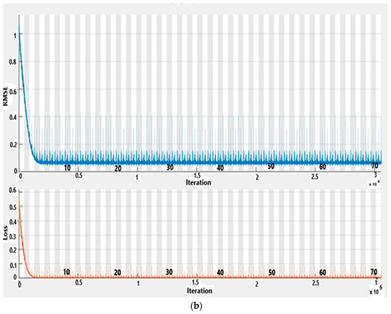
Figure 12.
CNN-BiLSTM-AM—RMSE and loss.
3.2.5. Hybrid Combination of CNN-LSTM
The main motivation for using the hybrid method on time series data is that a CNN model is good at extracting the key features and is also able to filter out noise that may be present in the input, while LSTM models are used to capture the sequence pattern information in the input data. Although CNN methods are employed to extract patterns of local trends and similar patterns in other sections of the time series data, they are not normally good at dealing with long temporal dependencies. This CNN weakness is taken care of by LSTM, as is dealing with temporal correlations using attributes in the training data [29]. The hybrid model exploits the strengths of both deep learning models, resulting in improved forecasting accuracy.
3.2.6. Performance Indicators
RMSE, mean square error (MSE), mean absolute percentage error (MAPE), and mean absolute error (MAE) are the commonly used performance indicators that are given in Equations (11)–(14). The decision to use one performance indicator depends on the intended results, the data being used, and the accuracy required.
where n is the number of data points, is the observed values, and is the predicted value. RMSE is used to measure the model’s error in predicting quantitative data and establishes the standard deviation of the prediction errors. It uses variance to assign more weight to errors with larger absolute values compared to errors with smaller absolute values. RMSE is effective in assessing the model’s error data and is concentrated around the line of best fit. When the samples are large enough and the error distribution is Gaussian, RMSE tends to be more appropriate to use. RMSE avoids the use of absolute values and is preferred in mathematical computations. MAE is an indicator of areas between the forecast value and the observed value, and it assigns the same weights to all errors. MAPE determines the prediction accuracy in model forecasting. MSE is a risk function related to the expected value of the squared error loss and is an average of the squared value of the difference between the predicted outcome and the actual outcome. The closer the MSE value is to zero, the better the quality and superiority of the model’s prediction capabilities. The selection of the most superior performance varies and depends on different researchers and the task they are working on. RMSE is used in this paper since it is the most appropriate and has better results.
Accuracy is a performance indicator that measures the proportion of correct predictions made by the model and is suitable for balanced datasets with equally represented classes as determined by the mathematical expression .
4. Results and Discussions
The same dataset is applied to five other algorithms, and the results are compared with the proposed hybrid model. These models are CNN, LSTM, BiLSTM, CNN-LSTM, CNN-BiLSTM, and CNN-BiLSTM-AM, and their prediction performances are shown in Table 1. The proposed CNN-BiLSTM-AM hybrid model has the best performance and minimum prediction error. RMSE and loss functions against iteration plots for CNN-BiLSTM-AM model performance are shown in Figure 12. Plotting RMSE against iteration in machine learning or optimization shows how the error changes throughout training or optimization. Initially, RMSE typically decreases rapidly as the model improves its predictions. Eventually, the rate of decrease slows, and RMSE may stabilize, indicating convergence. A rising RMSE on a validation dataset while the training RMSE continues to decrease suggests overfitting, prompting techniques like early stopping to prevent it. Overall, this visualization offers insights into training progress, convergence, and potential overfitting, aiding in the optimization of machine learning models. Plotting the loss against iteration in machine learning or optimization demonstrates how the loss function evolves during training or optimization. Initially, the loss typically decreases rapidly as the model learns from the data, indicating improvement in predictions. Over time, the rate of decrease may slow down, and the loss may stabilize, signifying convergence. A rising loss on a validation dataset while the training loss decreases suggests overfitting, prompting techniques like early stopping to prevent it. In essence, this visualization provides crucial insights into training progress, convergence, and potential overfitting, guiding the optimization of machine learning models.

Table 1.
Comparison of six methods prediction accuracy and performance evaluation indices.
For the RMSE graph, the y-axis is and the loss graph y-axis is . The network training cycle had 430 epochs and completed 43,000 iterations with a piecewise learning rate of 1exp (−12), and (a) shows 100% training complete while (b) is 70% complete. CNN-BiLSTM-AM offered superior accuracy by leveraging automated feature extraction, capturing temporal dependencies, focusing attention, enabling end-to-end learning, and ensuring adaptability compared to traditional methods.
Figure 13 shows CNN-BiLSTM RMSE and loss curves. The network training cycle had 430 epochs and completed 43,000 iterations with a piecewise learning rate of 1exp (−12), and (a) shows 100% training complete while (b) is 70% complete. RMSE and loss start to fall at epoch 3. An “epoch” in machine learning signifies one complete iteration through the entire training dataset during neural network training. It involves processing all data batches to adjust model parameters based on computed errors. Multiple epochs are typically needed for effective model training, with validation performed after each epoch to monitor progress and prevent overfitting.
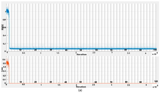
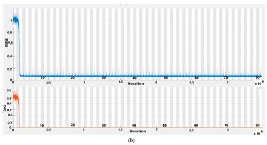
Figure 13.
CNN-BiLSTM—RMSE and loss.
Both RMSE and loss progressively decreased as the iterations increased. An indication measure of how a model can predict the expected outcome is called a loss function. A loss function is a commonly used metric to evaluate a model’s misclassification rate, i.e., the proportion of incorrect predictions. The deep learning network learns by means of the loss function. The loss function tends to be large when the predictions deviate significantly from the actual results. Optimization algorithms are used to ensure that the loss function learns to minimize the error in the prediction process. In general, loss functions are classified into two major categories, namely, regression losses and classification losses. In our work, the loss function is a regression loss because it is used to predict continuous values.
The trained network is tested by forecasting multiple harmonics in the future. The network would predict time steps one at a time, then update the network state at each prediction, i.e., the previous prediction is used as an input function for the current prediction. A large harmonics data and Intel Core i7 CPU are used. The Intel Core i7 processor is an industry-leading CPU in terms of its performance for discrete-level graphics and AI acceleration and predictions, as well as the RMSE is computed faster.
The results are in line with expectations. CNN has a fast training time and makes superior predictions when dealing with images instead of time series data. LSTM’s prediction performance on time series data is better than CNN’s prediction performance on time series data. BiLSTM’s prediction performance is better than LSTM’s since it extracts information from both forward and reverse directions. CNN-BiLSTM’s prediction is superior to that of CNN-LSTM. These hybrid models combine the advantages of either model, resulting in faster training times and better performance. Adding the attention mechanism to the CNN-BiLSTM model, which is the focus of this paper, further improves the prediction accuracy, as shown in Figure 14. In (a), the prediction in blue closely follows the expected in red; (b) shows the harmonics data; and (c) shows that the prediction in red closely follows the expected. The model’s prediction accuracy is superior. The proposed hybrid model achieved excellent results in the prediction of harmonics.
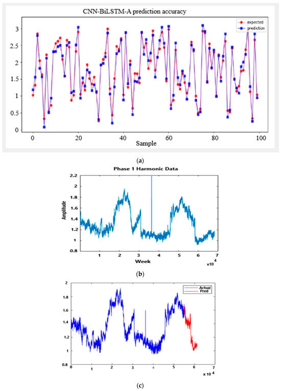
Figure 14.
CNN-BiLSTM A model predication accuracy.
The superiority of the proposed model is further shown in Table 1, where it is compared to the five other models. The table compares model prediction accuracy and RMSE.
The combination of CNNs, BiLSTMs, and attention mechanisms (AMs) can improve accuracy for the prediction of load harmonics compared to traditional methods in several ways:
- (i)
- CNN (feature extraction): Traditional methods often rely on handcrafted features or simplistic transformations of the input data. In contrast, CNNs can automatically learn hierarchical representations of the data, capturing both local and global features that are relevant to load harmonics. This allows the model to adapt more effectively to the complexity of the data and extract features that may not be apparent through manual analysis.
- (ii)
- BiLSTM (capturing temporal dependencies): Load harmonics data are inherently sequential, with complex temporal dependencies between data points. BiLSTMs are designed to capture such dependencies by processing the data bidirectionally, enabling the model to learn patterns across different time scales. This ability to capture long-range dependencies can lead to more accurate predictions compared to traditional methods that may struggle with capturing temporal dynamics effectively.
- (iii)
- Attention Mechanism: The attention mechanism further enhances the model’s ability to focus on relevant parts of the input sequence. In the context of load harmonics prediction, certain time periods or frequency components may be more critical for accurate forecasting. By dynamically adjusting the importance of different parts of the input sequence, the attention mechanism allows the model to prioritize information that is most relevant to the prediction task, leading to improved accuracy.
- (iv)
- End-to-End Learning: The CNN-BiLSTM-AM architecture facilitates end-to-end learning, where the model learns directly from the raw input data to make predictions. Traditional methods often involve multiple stages of preprocessing and feature engineering, which can introduce manual errors and may not fully capture the complexity of the data. By learning directly from the raw data, the CNN-BiLSTM-AM model can leverage the full information content of the input sequence, potentially leading to more accurate predictions.
- (v)
- Adaptability and Generalization: CNN-BiLSTM-AM models are highly adaptable and can generalize well to unseen data. Traditional methods may rely on assumptions or simplifications that limit their applicability to diverse datasets or changing conditions. The flexibility of deep learning models allows them to adapt to different data distributions and environmental factors, leading to more robust and accurate predictions across a wide range of scenarios.
Overall, the CNN-BiLSTM-AM architecture offers significant advantages over traditional methods for load harmonics prediction, including improved feature representation, better capture of temporal dependencies, enhanced attention mechanisms, end-to-end learning, and increased adaptability and generalization capabilities. These advantages contribute to higher accuracy and more reliable predictions in practical applications.
The hybrid model, consisting of CNN-BiLSTM-AM, exhibits optimal performance with minimal prediction error, as evidenced by the RMSE and loss function plots against iterations presented in Figure 12. In the RMSE graph, the y-axis is scaled by 1016, while the Loss graph y-axis is scaled by 1033. The network underwent 430 epochs, completing 43,000 iterations with a piecewise learning rate of 1exp(−12). Subplot (a) indicates 100% training completion, while subplot (b) represents 70% completion.
Figure 13 showcases the RMSE and loss curves for CNN-BiLSTM. Similar to the previous case, the network underwent 430 epochs, completing 43,000 iterations with a piecewise learning rate of 1exp(−12). Subplot (a) denotes 100% training completion, and subplot (b) signifies 70% completion. Notably, both the RMSE and loss curves begin to decline at epoch 3, indicating the model’s improving predictive capabilities.
The reduction in both RMSE and loss metrics continues as iterations progress. The loss function serves as a metric for evaluating misclassification rates, reflecting the proportion of incorrect predictions. Optimization algorithms ensure that the loss function minimizes prediction errors during the learning process.
Comparing individual model performances, CNN demonstrates rapid training for image-related tasks, while LSTM outperforms CNN in time series data prediction. BiLSTM, by considering information in both forward and reverse directions, surpasses LSTM. The hybrid CNN-BiLSTM model excels over CNN-LSTM, offering faster training and enhanced performance. The CNN-BiLSTM-AM model is validated using methods like holdout, cross-validation, time series validation, and stratified sampling. Given the time series nature and complexity of the harmonics data, time series validation methods were selected. This approach involves training the model on past data and validating it on future data using a rolling or expanding window approach. Other validation methods, include Nested Cross-Validation, Holdout with Stratified Sampling, Bootstrapping, Leave-One-Out Cross-Validation (LOOCV), Holdout Validation, and Cross-Validation.
The introduction of the attention mechanism in the CNN-BiLSTM model, highlighted in this study, further enhances prediction accuracy, as depicted in Figure 14. Subplot (a) illustrates the close alignment between the blue prediction curve and the red expected curve. Subplot (b) displays harmonics data, and subplot (c) showcases the red prediction closely matching the expected data, emphasizing the superior accuracy of the model in predicting harmonics.
Table 1 reinforces the excellence of the proposed hybrid model by comparing it to five other models. The table provides a comprehensive overview of model prediction accuracy and RMSE, further supporting the superior performance of the proposed hybrid model in predicting harmonics.
The CNN-BiLSTM-AM model introduces novel contributions to electrical power system harmonics analysis by integrating CNNs for feature extraction, BiLSTMs for capturing temporal dependencies, and attention mechanisms for focusing on relevant harmonic components. This integrated framework enhances the accuracy and interpretability of harmonic analysis, potentially improving detection and mitigation strategies for harmonic distortions in power systems.
In electrical engineering, the CNN-BiLSTM-AM architecture has various practical applications:
- (i)
- Power Quality Analysis:
- Voltage Sag/Swell Detection: Detect and classify voltage disturbances with CNNs, BiLSTMs, and attention mechanisms.
- Harmonic Analysis: Assess power quality and harmonic distortion using CNNs, BiLSTMs, and attention mechanisms.
- (ii)
- Power Grid Monitoring and Control:
- Fault Detection: Detect anomalies in power transmission systems using CNNs, BiLSTMs, and attention mechanisms.
- Load Forecasting: Predict future electricity demand by analyzing historical load data with CNNs, BiLSTMs, and attention mechanisms.
- (iii)
- Smart Grid Optimization:
- Energy Management: Optimize energy distribution and consumption in smart grids with CNNs, BiLSTMs, and attention mechanisms.
- Renewable Energy Integration: Integrate renewable energy sources efficiently using CNNs, BiLSTMs, and attention mechanisms.
- (iv)
- Electrical Equipment Maintenance:
- Predictive Maintenance: Predict and prevent equipment failures with CNNs, BiLSTMs, and attention mechanisms.
- Condition Monitoring: Continuously monitor equipment health and performance using CNNs, BiLSTMs, and attention mechanisms.
These applications highlight how the CNN-BiLSTM-AM architecture can be applied in electrical engineering for various tasks such as monitoring, control, optimization, and maintenance.
The CNN-BiLSTM-AM model, while powerful for sequence modeling, faces notable limitations. Its computational complexity demands substantial resources for training and inference, restricting its deployment in resource-constrained environments. Moreover, large labeled datasets are necessary for optimal performance, posing challenges for applications with limited data availability. Hyperparameter tuning is time-consuming and expertise-intensive, crucial for achieving model effectiveness, while the model’s complex architecture hinders interpretability, impacting its suitability for transparent decision-making contexts. Overfitting is a risk, especially with small datasets or overly complex architectures, and training time can be lengthy, necessitating acceleration techniques for efficiency. Domain specificity may require retraining or fine-tuning, and imbalanced datasets can undermine performance, necessitating additional mitigation strategies. Understanding and addressing these limitations are essential for effective utilization of the CNN-BiLSTM-AM model across diverse applications.
Future work on the CNN-BiLSTM-AM hybrid model could involve hyperparameter tuning, adjusting model architecture, exploring ensemble methods, and optimizing for real-time applications. Continuous evaluation and refinement of the model along these suggested directions, can enhance its adaptability and effectiveness. One potential avenue for future work involves the development of the demand-side subsystem within the electrical power system. This would entail integrating the trained model and evaluating its impact. A comparative analysis would then be conducted between the demand-side subsystem with and without the model to assess its effectiveness.
5. Conclusions
This work proposes a deep learning CNN-BiLSTM-AM hybrid model for harmonics prediction. The historical data were collected at a chocolate manufacturing factory in East London, South Africa, and the main source of harmonics is the variable speed drives. The prediction methodology has the following steps: The dataset is divided into training data and test data, and the data are apportioned as 80% and 20%, respectively. The proposed CNN-BiLSTM-AM model prediction performance is compared with five other algorithms. The hybrid model exploits the strengths of both deep learning models, resulting in improved forecasting accuracy. RMSE is used to measure the method’s prediction performance. Based on the results, the CNN-BiLSTM-AM model produces superior results compared to the other models. The superiority of the individual algorithms and the attention mechanism all put together greatly improved prediction accuracy, lowered the RMSE to 0.0000002215, and achieved an accuracy of 92.3569%.
Author Contributions
Conceptualization, methodology, software, validation, formal analysis, investigation, resources, writing—original draft preparation, data curation, E.M.K. Writing—review and editing visualization, E.M.K., A.N.H. and T.C.S. project administration, funding acquisition, A.N.H. and T.C.S. All authors have read and agreed to the published version of the manuscript.
Funding
This research received no external funding.
Data Availability Statement
Not application.
Conflicts of Interest
The authors declare no conflict of interest.
References
- de Jonge, B.; Scarf, P.A. A review on maintenance optimization. Eur. J. Oper. Res. 2020, 285, 805–824. [Google Scholar] [CrossRef]
- Mancuso, P.; Piccialli, V.; Sudoso, A.M. A machine learning approach for forecasting hierarchical time series. Expert Syst. Appl. 2021, 182, 115102. [Google Scholar] [CrossRef]
- Chen, F.; Chen, J.; Guo, P.; Xue, W.; Zheng, L.; Chen, B. A Fault Prediction Of Equipment Based On CNN-LSTM Network. In Proceedings of the 2019 IEEE International Conference on Energy Internet (ICEI), Nanjing, China, 27–31 May 2019; pp. 537–541. [Google Scholar] [CrossRef]
- Alhussein, M.; Aurangzeb, K.; Haider, S.I. Hybrid CNN-LSTM Model for Short-Term Individual Household Load Forecasting. IEEE Access 2020, 8, 180544–180557. [Google Scholar]
- Tan, Z.; Pan, P. Network Fault Prediction Based on CNN-LSTM Hybrid Neural Network. In Proceedings of the 2019 International Conference on Communications, Information System and Computer Engineering (CISCE), Haikou, China, 5–7 July 2019. [Google Scholar] [CrossRef]
- Motepe, S.; Hasan, A.N.; Twala, B.; Stopforth, R. Power Distribution Networks Load Forecasting Using Deep Belief Networks: The South African. In Proceedings of the 2019 IEEE Jordan International Joint Conference on Electrical Engineering and Information Technology, Amman, Jordan, 9–11 April 2019; pp. 507–512. [Google Scholar]
- Gellert, A.; Fiore, U.; Florea, A.; Chis, R.; Palmieri, F. Forecasting Electricity Consumption and Production in Smart Homes through Statistical Methods. Sustain. Cities Soc. 2022, 76, 103426. [Google Scholar] [CrossRef]
- Kuyumani, E.M.; Hasan, A.N.; Sbongwe, T. Harmonic current and voltage monitoring using artificial neural network. In Proceedings of the 2020 International Conference on Artificial Intelligence, Big Data, Computer and Data Communication System (icABCD), Durban, South Africa, 6–7 August 2020. [Google Scholar] [CrossRef]
- Kuyunani, E.M.; Hasan, A.N.; Shongwe, T. Improving voltage harmonics forecasting at a wind farm using deep learning techniques. In Proceedings of the 2021 IEEE 30th International Symposium on Industrial Electronics (ISIE), Kyoto, Japan, 20–23 June 2021; pp. 1–6. [Google Scholar] [CrossRef]
- Kuyumani, E.M.; Hasan, A.N.; Shongwe, T. A Hybrid Model Based on CNN-LSTM to Detect and Forecast Harmonics: A Case Study of an Eskom Substation in South Africa. Electr. Power Compon. Syst. 2023, 51, 746–760. [Google Scholar] [CrossRef]
- Garcia, C.I.; Grasso, F.; Luchetta, A.; Piccirilli, M.C.; Paolucci, L.; Talluri, G. A Comparison of Power Quality Disturbance Detection and Classification Methods Using CNN, LSTM and CNN-LSTM. Appl. Sci. 2020, 10, 6755. [Google Scholar] [CrossRef]
- Khan, S.; Nagar, S.; Meena, M.; Singh, B. Comparison between SPWM and OHSW technique for harmonic elimination in 15 level multilevel inverter. In Proceedings of the IEEE International Conference on Information, Communication and Instrumentation Control (ICICIC), Indore, India, 17–19 August 2017; Volume 2018, pp. 1–5. [Google Scholar] [CrossRef]
- Gupta, H.; Yadav, A.; Maurya, S. Multi carrier PWM and selective harmonic elimination technique for cascade multilevel inverter. In Proceedings of the IEEE 2nd International Conference on Advances in Electrical, Electronics, Information, Communication and Bio-Informatics (AEEICB16), Chennai, India, 27–28 February 2016; pp. 98–102. [Google Scholar] [CrossRef]
- Wang, Z.; Li, Y.; Zhang, H. Harmonic detection method based on windowed double-spectrum interpolation FFT. In Proceedings of the2019 International Conference on Robots & Intelligent System (ICRIS), Haikou, China, 15–16 June 2019; pp. 425–427. [Google Scholar] [CrossRef]
- Wen, H.; Zhang, J.; Yao, W.; Tang, L. FFT-Based Amplitude Estimation of Power Distribution Systems Signal Distorted by Harmonics and Noise. IEEE Trans. Ind. Inform. 2018, 14, 1447–1455. [Google Scholar] [CrossRef]
- Shuai, Z.; Zhang, J.; Tang, L.; Teng, Z.; Wen, H. Frequency Shifting and Filtering Algorithm for Power System Harmonic Estimation. IEEE Trans. Ind. Inform. 2019, 15, 1554–1565. [Google Scholar] [CrossRef]
- Zhao, H.; Jin, T.; Wang, S.; Sun, L. A Real-Time Selective Harmonic Elimination Based on a Transient-Free Inner Closed-Loop Control for Cascaded Multilevel Inverters. IEEE Trans. Power Electron. 2016, 31, 1000–1014. [Google Scholar] [CrossRef]
- Aljendy, R.; Sultan, H.M.; Al-Sumaiti, A.S.; Diab, A.A.Z. “Harmonic Analysis in Distribution Systems Using a Multi-Step Prediction with NARX. In Proceedings of the 46th Annual Conference of the IEEE Industrial Electronics Society (IECON), Singapore, 18–21 October 2020; pp. 2545–2550. [Google Scholar] [CrossRef]
- Liu, J.; Shao, Y.; Qin, X.; Lu, X. Inter-harmonics Parameter Detection Based on Interpolation FFT and Multiple Signal Classification Algorithm. In Proceedings of the 2019 31st Chinese Control and Decision Conference (CCDC), Nanchang, China, 3–5 June 2019; pp. 4691–4696. [Google Scholar] [CrossRef]
- Wang, H.; Yang, T.; Han, Q.; Luo, Z. Approach to the Quantitative Diagnosis of Rolling Bearings Based on Optimized VMD and Lempel–Ziv Complexity under Varying Conditions. Sensors 2023, 23, 4044. [Google Scholar] [CrossRef] [PubMed]
- Akpudo, U.E.; Hur, J.-W. A CEEMDAN-Assisted Deep Learning Model for the RUL Estimation of Solenoid Pumps. Electronics 2021, 10, 2054. [Google Scholar] [CrossRef]
- Wang, K.; Wang, C.; Wang, Y.; Luo, W.; Zhan, P.; Hu, Y.; Li, X. Time Series Classification via Enhanced Temporal Representation Learning. In Proceedings of the 2021 IEEE 6th International Conference on Big Data Analytics (ICBDA), Xiamen, China, 5–8 March 2021; pp. 188–192. [Google Scholar] [CrossRef]
- Wang, J.A.; Yang, M.; Wang, J.; Yang, M.; Wang, J. Adaptability of Financial Time Series Based on BiLSTM. Procedia Comput. Sci. 2022, 199, 18–25. [Google Scholar] [CrossRef]
- Masita, K.; Hasan, A.; Shongwe, T. Deep Learning in Object Detection: A Review. In Proceedings of the 2020 International Conference on Artificial Intelligence, Big Data, Computing and Data Communication Systems (icABCD), Durban, South Africa, 6–7 August 2020. [Google Scholar] [CrossRef]
- Deng, Y.; Wang, L.; Jia, H.; Tong, X.; Li, F. A Sequence-to-Sequence Deep Learning Architecture Based on Bidirectional GRU for Type Recognition and Time Location of Combined Power Quality Disturbance. IEEE Trans. Ind. Inform. 2019, 15, 4481–4493. [Google Scholar] [CrossRef]
- Kavianpour, P.; Kavianpour, M.; Ramezani, A. A CNN-BiLSTM Model with Attention Mechanism for Earthquake Prediction. J. Supercomput. 2023, 79, 19194–19226. [Google Scholar] [CrossRef]
- Khodayar, M.; Liu, G.; Khodayar, M.E. Deep Learning in Power Systems Research. CSEE J. Power Energy Syst. 2021, 7, 209–220. [Google Scholar] [CrossRef]
- Ali, A.; Hasan, A.N. Optimization of PV Model using Fuzzy- Neural Network for DC-DC converter Systems. In Proceedings of the 2018 9th International Renewable Energy Congress (IREC), Hammamet, Tunisia, 20–22 March 2018; pp. 1–6. [Google Scholar] [CrossRef]
- Yang, T.; Wang, H.; Aziz, S.; Jiang, H.; Peng, J. A Novel Method of Wind Speed Prediction by Peephole LSTM. In Proceedings of the 2018 International Conference on Power System Technology (POWERCON), Guangzhou, China, 6–8 November 2018; pp. 364–369. [Google Scholar] [CrossRef]
Disclaimer/Publisher’s Note: The statements, opinions and data contained in all publications are solely those of the individual author(s) and contributor(s) and not of MDPI and/or the editor(s). MDPI and/or the editor(s) disclaim responsibility for any injury to people or property resulting from any ideas, methods, instructions or products referred to in the content. |
© 2024 by the authors. Licensee MDPI, Basel, Switzerland. This article is an open access article distributed under the terms and conditions of the Creative Commons Attribution (CC BY) license (https://creativecommons.org/licenses/by/4.0/).