Transient Pressure Performance Analysis of Hydraulically Fractured Horizontal Well in Tight Oil Reservoir

Abstract

Utilizing the discrete fracture model (DFM), a transient flow model is established for fractured horizontal wells in tight oil reservoirs, accounting for threshold pressure gradient (TPG), stress sensitivity effect, hydraulic fracture parameters, and fracture distribution pattern. This model is solved using the finite-volume method (FVM), and an important sensitivity analysis is conducted. The findings reveal that the models incorporated by the threshold pressure gradient result in an upward trend in the pressure-derivative curve. As the threshold pressure gradient increases, this upward trend becomes more pronounced, rendering the distinction between flow regimes more challenging. The stress sensitivity effect predominantly impacts the pressure-derivative curve during the later flow period. Additionally, as the fracture half-length increases, the pressure performance of both fracture radial flow and formation radial flow becomes more difficult. Fracture conductivity has a significant influence during the early flow period, facilitating the identification of flow regimes with the trend of increasing fracture conductivity.

1. Introduction

As the key technology of tight oil reservoir development, multiple-hydraulic-fracture stimulation [1,2] can enlarge the accessible reservoir volume and improve well productivity significantly. To gain a deeper understanding of the impact of the fracturing and formation characteristics, it is imperative to research the transient flow model of fractured horizontal wells. Over the past few decades, numerous studies have been conducted in this field. Guo and Evans [3,4,5,6] utilized the source, Green’s function, and the superposition principle to derive solutions for fractured horizontal wells. Raghavan et al. [7] further explored the distinct response patterns of such wells by developing a mathematical model. Additionally, Zerzar et al. [8] introduced an analytical model specifically tailored for fractured horizontal wells in which semi-infinite, or anisotropic closed, homogenous, or naturally fractured systems have been considered for finite-conductivity, infinite-conductivity, and uniform-flux models. Al-Kobaisi et al. [9] introduced a hybrid model that integrated numerical and analytical techniques, dynamically linking a numerical fracture model with an analytical reservoir model. This approach allowed for a comprehensive analysis of the pressure-transient response in a horizontal well intersecting a finite-conductivity fracture. In addition, Wei et al. [10] examined the influence of turbulence on the pressure variation behavior of fluid flow and specifically focused on the fluid movement from the formation to the horizontal well with transverse fractures. Medeiros et al. [11] delved into the diagnostic analysis of pressure and pressure-derivative curves for fractured horizontal wells in inhomogeneous, locally fractured, and globally fractured reservoirs. Their findings revealed that the flow patterns in horizontal wells with transverse and longitudinal hydraulic fractures diverged primarily during the early and intermediate stages. Ozkan [12] employed the simplified trilinear flow model to simulate the transient pressure behavior and production patterns in fractured horizontal wells within unconventional reservoirs. Yao et al. [13] introduced a semi-analytical model leveraging Green’s function and the source/sink method, to present transient pressure analysis for multi-stage fractured horizontal wells in closed box-shaped reservoirs. Rbeawi et al. [14] derived solutions for fractured horizontal wells accounting for various fracture orientations, symmetries, and fracture propagation behaviors in isotropic or anisotropic formations with varying dimensions and spacing. Zhao et al. [15] utilized the source function to examine the transient pressure response of multiple-fractured horizontal wells in shale gas reservoirs, providing crucial insights into their performance. Yao et al. [16] derived an analytical solution for pressure dynamics in horizontal wells with multiple hydraulic fractures, leveraging the mirror-injection and superposition theorem given by the source/Green’s function method. Fan et al. [17] constructed a numerical composite-formation model for multiple-fractured horizontal wells, taking into account the stimulated reservoir volume (SRV). In their paper, three key zones were divided for the reservoir: hydraulic fracture zone, stimulated reservoir volume zone, and unstimulated matrix zone. Ren et al. [18] set up a transient pressure model of tight oil considering stress sensitive effect and double porosity model. In addition, the Laplace transform, perturbation transform, and superposition have been applied to solve the mathematical model.

The threshold pressure gradient (TPG) and stress sensitivity effect play pivotal roles in regulating fluid flow within tight oil reservoirs [19,20]. Song et al. [21] devised an experimental framework using a static approach to quantitatively assess the TPG within distinct wettability surface microchannels. Their findings demonstrated the TPG’s existence in microchannels. Zeng et al. [22] constructed an experimental apparatus to probe single-phase oil/water flow in ultra-low-permeability cores, leveraging a capillary flow meter for precise fluid volume measurements. Their study revealed that single-phase oil/water flow in these cores deviated from Darcy’s law, and a minimum threshold pressure gradient was widely observed for various fluids. Zhu et al. [23] conducted experimental research on the TPG’s occurrence conditions for gas transport in water-bearing tight gas reservoirs. Additionally, Davies et al. [24] presented several cases with a conceptual model of tight sandstone gas reservoirs, including stress-dependent permeability. Their results show that stress-dependent permeability should be accurately forecast to predict optimum production conditions. Shi et al. [25] explored the stress sensitivity effect of the Changqing tight gas reservoir, and a close exponential relationship between formation stress and rock permeability/porosity was obtained. In another study, Dautriat et al. [26] utilized an integrated approach combining hydrostatic and triaxial compression experiments, petrophysical analysis, high-resolution CMT imaging, and pore network simulations to simulate the mechanical impact of hydrostatic stress on rock properties in the linear deformation regime. Hence, the existence of the threshold pressure gradient (TPG) and stress sensitivity effect poses significant challenges in establishing a reliable well testing model for fractured horizontal wells in tight oil reservoirs because Darcy’s law fails to accurately describe fluid flow in these unique geological formations. Diwu et al. [27] proposed a new pressure superposition principle for shale and tight oil by considering TPG and different shut-in periods. Wu et al. [28] provided a simplified multi-linear transient pressure mathematical model considering TPG and the stress sensitivity effect. In their paper, six flow regimes were given, but wellbore storage effects were ignored.

Drawing upon the discrete fracture model, this study constructed a transient flow model specifically tailored for fractured horizontal wells within tight oil reservoirs. This model took into account crucial factors such as the threshold pressure gradient, stress sensitivity effects, fracture parameters, and their distribution patterns. Subsequently, the transient flow model was solved using the finite-volume method, and a comprehensive sensitivity analysis was conducted. This approach provides a more meaningful understanding of pressure performance for complex fluid flow behavior in tight oil reservoirs.

2. Transient Flow Model for a Fractured Horizontal Well in Tight Oil Reservoirs

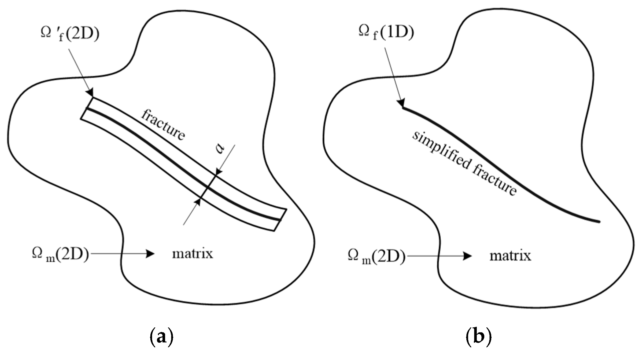
2.1. Physical Model

Drawing upon the fractured horizontal well configuration depicted in Figure 1 within a tight oil reservoir, several key assumptions should be given, as follows. The porous medium is assumed to be homogeneous, isotropic, and isothermal, ensuring consistency in its physical properties. Both the fluid and the rock are considered to be slightly compressible, and constant individual compressibility factors are considered. Moreover, the influence of stress sensitivity and wellbore storage is taken into account, capturing the dynamic interactions between the reservoir and the wellbore. The effects of gravity and capillary force are neglected to simplify the analysis. Meanwhile, it is assumed that the fractures penetrate the reservoir and are symmetric around the wellbore with a regular geometric distribution.

2.2. Mathematical Model for the Matrix System

The motion equation of a matrix porous medium in tight oil reservoirs, including TPG and the stress sensitivity effect, is as follows [27]:

$$v_{\mathrm{m}}=\{\begin{array}{ll}-\frac{k_0{e}^{\alpha \left(P-P_0\right)}}{\mu }\left(1-\frac{G}{\left|\nabla P\right|}\right)\nabla P& \left|\nabla P\right|>G\\ 0& \left|\nabla P\right|\le G\end{array}$$

(1)

where v_m is the fluid flow velocity in the matrix porous medium, cm/s; k₀ is the initial formation permeability, μm²; α is the permeability modulus, 10 MPa⁻¹; G is the TPG, 10⁻¹ MPa/cm; μ is the fluid viscosity, mPa·s; P₀ is the initial formation pressure, 10⁻¹ MPa; and P is the formation pressure, 10⁻¹ MPa.

The rock state equation of elastic porous media is as follows [29]:

$$\varphi ={\varphi }_0+C_{\mathrm{f}}\left(P-P_0\right)$$

(2)

where $\varphi$ is the porosity of the matrix porous medium; ${\varphi }_0$ is the initial porosity of the matrix porous medium; and C_f is the rock compressibility, 10 MPa⁻¹.

The state equation of the formation fluid is the following [29]:

$$\rho ={\rho }_0{e}^{C_{\mathrm{l}}\left(P-P_0\right)}$$

(3)

where ρ is the fluid density, g/cm³; ρ₀ is the initial fluid density, g/cm³; and C_l is the fluid compressibility, 10 MPa⁻¹.

The mass conservation equation is the following [29]:

$$\frac{\partial \left(\rho \varphi \right)}{\partial t}+\mathrm{div}\left(\rho v_{\mathrm{m}}\right)=0$$

(4)

Equation (5) is obtained based on Equations (2)–(4):

$$-\mathrm{div}\left(v_{\mathrm{m}}\right)-C_{\mathrm{l}}{v}_{\mathrm{m}}\nabla P=C_{\mathrm{t}}\frac{\partial P}{\partial t}$$

(5)

By substituting Equation (1) into the second term on the left of Equation (5), one can obtain the following:

$$C_{\mathrm{l}}{v}_{\mathrm{m}}\nabla P=\{\begin{array}{ll}-\frac{k{C}_{\mathrm{l}}}{\mu }\left[{\left(\nabla P\right)}^2-\frac{G{\left(\nabla P\right)}^2}{\left|\nabla P\right|}\right]& \left|\nabla P\right|>G\\ 0& \left|\nabla P\right|\le G\end{array}$$

(6)

where k is the effective permeability, $k=k_0{e}^{\alpha \left(P-P_0\right)}$.

The $\frac{k{C}_{\mathrm{l}}}{\mu }{\left(\nabla P\right)}^2$ and $\frac{k{C}_{\mathrm{l}}}{\mu }G\frac{{\left(\nabla P\right)}^2}{\left|\nabla P\right|}$ in Equation (6) can be ignored as they are too small and have a different sign, which means that the $C_{\mathrm{l}}{v}_{\mathrm{m}}\nabla P$ in Equation (6) can also be ignored. Then, the governing equation of the matrix porous medium in a tight oil reservoir becomes the following:

$$-\mathrm{div}\left(v_{\mathrm{m}}\right)=C_{\mathrm{t}}\frac{\partial P}{\partial t}$$

(7)

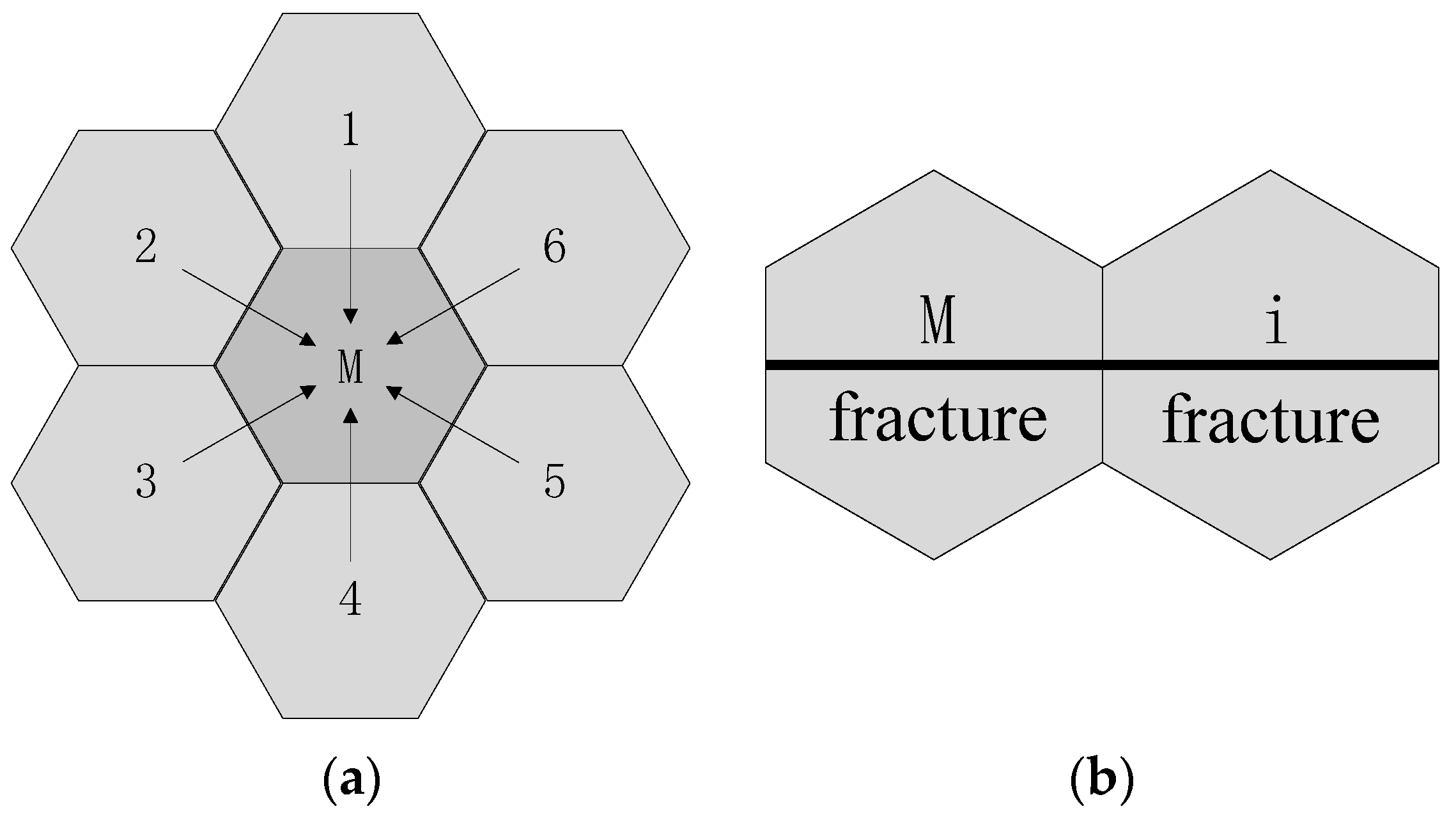
2.3. Mathematical Model for Fracture System Based on DFM

We take the fractures as one-dimensional entities based on the discrete fracture model [30,31,32,33,34] (Figure 2).

Based on the above assumptions, the motion equation of the fracture porous medium is as follows:

$$v_{\mathrm{f}}=-\frac{k_{\mathrm{f}}}{\mu }\mathrm{grad}{P}_{\mathrm{f}}$$

(8)

where v_f is the velocity in the fracture, cm/s; k_f is the fracture permeability, μm²; and P_f is the fracture pressure, 10⁻¹ MPa.

Some researchers [35,36] have proven that the compressibility of the fracture porous medium can be ignored; hence, the governing equation is the following:

$$\mathrm{div}\left(v_{\mathrm{f}}\right)=0$$

(9)

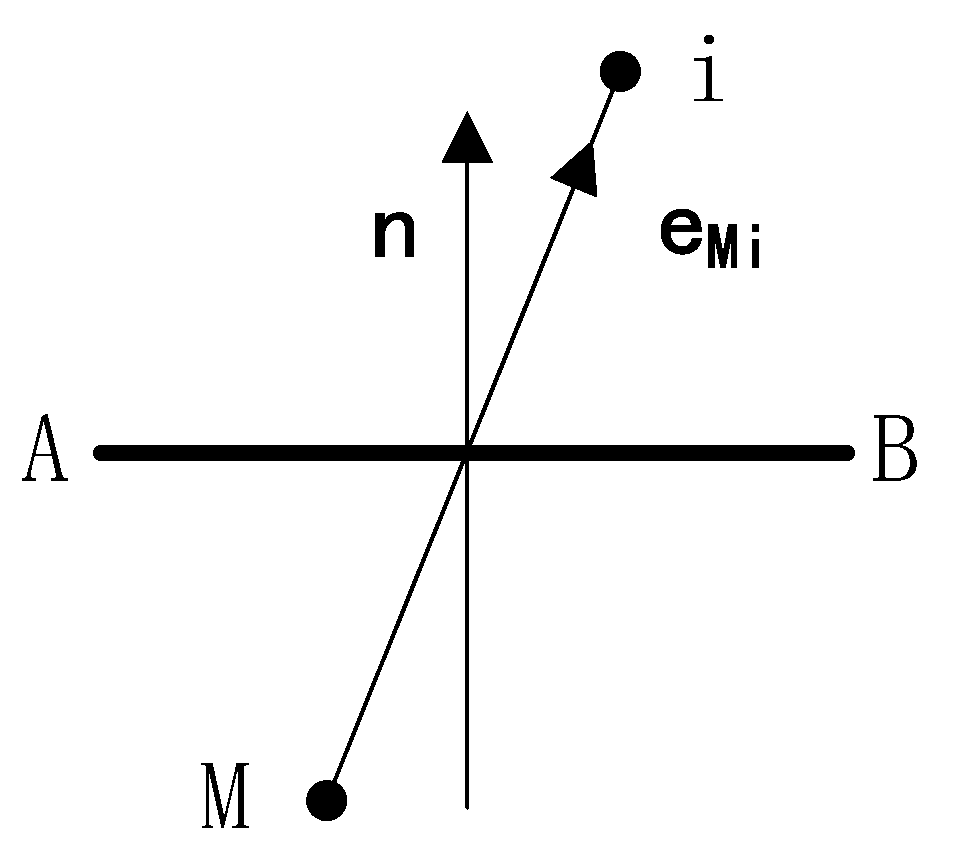
2.4. Mathematical Model for the Inner Boundary

The fluid flows from the fractures into the horizontal wellbore. The relationship between the surface production rate and the sandface rate when considering the wellbore storage is as follows:

Production well:

$$q-q_{\mathrm{b}}=-\frac{C}{B}\frac{\partial P_{\mathrm{wf}}}{\partial t}$$

(10)

Injection well:

$$q-q_{\mathrm{b}}=\frac{C}{B}\frac{\partial P_{\mathrm{wf}}}{\partial t}$$

(11)

where q is the surface production rate (std), cm³/s; q_b is the sandface rate, cm³/s; C is the wellbore storage coefficient, cm³/10⁻¹ MPa; B is the formation volume factor; and P_wf is the bottomhole pressure, 10⁻¹ MPa.

3. Numerical Solution for the Well Test Model

The new well test model can be solved numerically by FVM for fractured horizontal wells in tight oil reservoirs. Figure 3 represents the schematic of the cell vertex network model.

Figure 2 represents the notion that, if the global region is Ω, the matrix region is Ω_m, the fracture region is Ω_f, then the global region can be presented as follows:

$$\mathsf{\Omega }={\mathsf{\Omega }}_{\mathrm{m}}+{{\mathsf{\Omega }}^{\prime }}_{\mathrm{f}}={\mathsf{\Omega }}_{\mathrm{m}}+a{\mathsf{\Omega }}_{\mathrm{f}}$$

(12)

where a is the fracture aperture, cm.

(1)

The matrix region

We integrate Equation (7) to obtain Equation (13) for the matrix zone:

$${\displaystyle \underset{{\mathsf{\Omega }}_{\mathrm{m}}}{\int }-\mathrm{div}\left(v_{\mathrm{m}}\right)}\mathrm{d}{\mathsf{\Omega }}_{\mathrm{m}}={\displaystyle \underset{{\mathsf{\Omega }}_{\mathrm{m}}}{\int }{C}_{\mathrm{t}}\frac{\partial P}{\partial t}}\mathrm{d}{\mathsf{\Omega }}_{\mathrm{m}}$$

(13)

We then transform the left term in Equation (13) as the integration over the control volume (CV) surface based on Gauss’ Divergence Theorem.

$${\displaystyle \underset{A_{\mathrm{m}}}{\iint }-v_{\mathrm{m}}·n}\mathrm{d}{A}_{\mathrm{m}}={\displaystyle \underset{{\mathsf{\Omega }}_{\mathrm{m}}}{\int }{C}_{\mathrm{t}}\frac{\partial P}{\partial t}}\mathrm{d}{\mathsf{\Omega }}_{\mathrm{m}}$$

(14)

For CV_M, the physical meaning of the left term of Equation (14) is the total flux from neighboring CVs. The schematic of unit vector n and unit vector e_Mi of v_m is represented in Figure 4.

When $n·e_{\mathrm{Mi}}\left|P_{\mathrm{i}}-P_{\mathrm{M}}\right|/l_{\mathrm{Mi}}>G$, the flux from CV_i into CV_M is as follows:

$$Q_{\mathrm{mMi}}=T_{\mathrm{Mi}}{\lambda }_{\mathrm{Mi}}\left(P_{\mathrm{i}}-P_{\mathrm{M}}\right)-T_{\mathrm{GMi}}G{\lambda }_{\mathrm{Mi}}\left(P_{\mathrm{i}}-P_{\mathrm{M}}\right)/\left|P_{\mathrm{i}}-P_{\mathrm{M}}\right|$$

(15)

where ${\lambda }_{\mathrm{Mi}}=\left(k_{\mathrm{M}}+k_{\mathrm{i}}\right)/2\mu$, $k_{\mathrm{M}}=k_0{e}^{\alpha \left(P_{\mathrm{M}}-P_0\right)}$, $k_{\mathrm{i}}=k_0{e}^{\alpha \left(P_{\mathrm{i}}-P_0\right)}$, $T_{\mathrm{Mi}}=h{l}_{\mathrm{AB}}n·e_{\mathrm{Mi}}/l_{\mathrm{Mi}}$, $T_{\mathrm{GMi}}=h{l}_{\mathrm{AB}}$, h is the reservoir height, l_AB is the side length of CV_i and CV_M contact, l_Mi is the distance between the CV_M centroid and the CV_i centroid, $n$ is the unit normal vector to the control interface, and $e_{\mathrm{Mi}}$ is the unit vector along the direction of the line joining the centroids of CV_M and CV_i.

Governing Equation (16) can be obtained by discretizing Equation (15) when $n·e_{\mathrm{Mi}}\left|P_{\mathrm{i}}-P_{\mathrm{M}}\right|/l_{\mathrm{Mi}}>G$:

$${\displaystyle \sum _{i=1}^N{T}_{\mathrm{Mi}}\frac{k_{\mathrm{M}}^n+k_{\mathrm{i}}^n}{2\mu }\left(P_{\mathrm{i}}^{n+1}-P_{\mathrm{M}}^{n+1}\right)}=C_{\mathrm{tM}}\Delta V_{\mathrm{M}}\frac{P_{\mathrm{M}}^{n+1}-P_{\mathrm{M}}^n}{\Delta t^{n+1}}+{\displaystyle \sum _{i=1}^N{T}_{\mathrm{GMi}}G\frac{k_{\mathrm{M}}^n+k_{\mathrm{i}}^n}{2\mu }\frac{P_{\mathrm{i}}^n-P_{\mathrm{M}}^n}{\left|P_{\mathrm{i}}^n-P_{\mathrm{M}}^n\right|}}$$

(16)

where N is the number of neighboring CVs of CV_M, $k_{\mathrm{M}}^n=e^{\alpha \left(P_{\mathrm{M}}^n-P_0\right)}$, and $k_{\mathrm{i}}^n=e^{\alpha \left(P_{\mathrm{i}}^n-P_0\right)}$.

The numerical discrete scheme of Equation (16) is as follows:

$${\displaystyle \sum _{i=1}^N{T}_{\mathrm{Mi}}\frac{k_{\mathrm{M}}^n+k_{\mathrm{i}}^n}{2\mu }{P}_{\mathrm{i}}^{n+1}}-\left({\displaystyle \sum _{i=1}^N{T}_{\mathrm{Mi}}\frac{k_{\mathrm{M}}^n+k_{\mathrm{i}}^n}{2\mu }}+\frac{C_{\mathrm{tM}}\Delta V_{\mathrm{M}}}{\Delta t^{n+1}}\right)P_{\mathrm{M}}^{n+1}=-\frac{C_{\mathrm{tM}}\Delta V_{\mathrm{M}}}{\Delta t^{n+1}}{P}_{\mathrm{M}}^n+{\displaystyle \sum _{i=1}^N{T}_{\mathrm{GMi}}G\frac{k_{\mathrm{M}}^n+k_{\mathrm{i}}^n}{2\mu }\frac{P_{\mathrm{i}}^n-P_{\mathrm{M}}^n}{\left|P_{\mathrm{i}}^n-P_{\mathrm{M}}^n\right|}}$$

(17)

The flux from CV_i into CV_M is zero when $n·e_{\mathrm{Mi}}\left|P_{\mathrm{i}}-P_{\mathrm{M}}\right|/l_{\mathrm{Mi}}\le G$.

(2)

The fracture region

We integrate Equation (9) (fracture region) into Equation (18):

$$a{\displaystyle \underset{{\mathsf{\Omega }}_{\mathrm{f}}}{\int }-\mathrm{div}\left(v_{\mathrm{f}}\right)}\mathrm{d}{\mathsf{\Omega }}_{\mathrm{f}}=0$$

(18)

We transform the term on the left terms of Equation (18) as the integration over the fracture segments of the control volume surface, which can be shown as Equation (19):

$$a{\displaystyle \underset{A_{\mathrm{f}}}{\iint }-v_{\mathrm{f}}}\mathrm{d}{A}_{\mathrm{f}}=0$$

(19)

For CV_M, the physical meaning of the left term in Equation (19) is the total flux from the neighboring CVs through fractures.

The flux from CV_i into CV_M is as follows:

$$Q_{\mathrm{fMi}}=T_{\mathrm{fMi}}{\lambda }_{\mathrm{f}}\left(P_{\mathrm{i}}-P_{\mathrm{M}}\right)$$

(20)

where ${\lambda }_{\mathrm{f}}=k_{\mathrm{f}}/\mu$ and $T_{\mathrm{fMi}}=ah/l_{\mathrm{Mi}}$.

The following numerical scheme of Equation (21) of CV_M, which contains a fracture, can be obtained using Equations (17)–(20):

$$\begin{array}{l}{\displaystyle \sum _{i=1}^N{T}_{\mathrm{Mi}}\frac{k_{\mathrm{M}}^n+k_{\mathrm{i}}^n}{2\mu }{P}_{\mathrm{i}}^{n+1}}-\left({\displaystyle \sum _{i=1}^N{T}_{\mathrm{Mi}}\frac{k_{\mathrm{M}}^n+k_{\mathrm{i}}^n}{2\mu }}+\frac{C_{\mathrm{tM}}\Delta V_{\mathrm{M}}}{\Delta t^{n+1}}\right)P_{\mathrm{M}}^{n+1}+{\displaystyle \sum _{i=1}^{N_{\mathrm{f}}}{T}_{\mathrm{fMi}}{\lambda }_{\mathrm{f}}{P}_{\mathrm{i}}^{n+1}}-{\displaystyle \sum _{i=1}^{N_{\mathrm{f}}}{T}_{\mathrm{fMi}}{\lambda }_{\mathrm{f}}{P}_{\mathrm{M}}^{n+1}}\\ =-\frac{C_{\mathrm{tM}}\Delta V_{\mathrm{M}}}{\Delta t^{n+1}}{P}_{\mathrm{M}}^n+{\displaystyle \sum _{i=1}^N{T}_{\mathrm{GMi}}G\frac{k_{\mathrm{M}}^n+k_{\mathrm{i}}^n}{2\mu }\frac{P_{\mathrm{i}}^n-P_{\mathrm{M}}^n}{\left|P_{\mathrm{i}}^n-P_{\mathrm{M}}^n\right|}}\end{array}$$

(21)

where N_f is the number of CVs connected to CV_M through the fracture.

(3)

The inner boundary’s treatment

Taking a production well as an example, the centroid of CV_M, which contains a fracture, is on the inner boundary. This numerical scheme can be given as follows:

$$T_{\mathrm{fMi}}{\lambda }_{\mathrm{f}}{P}_{\mathrm{i}}^{n+1}-\left(T_{\mathrm{fMi}}{\lambda }_{\mathrm{f}}+\frac{C_{\mathrm{tM}}\Delta V_{\mathrm{M}}}{\Delta t^{n+1}}\right)P_{\mathrm{M}}^{n+1}-q_{\mathrm{M}}^{n+1}=-\frac{C_{\mathrm{tM}}\Delta V_{\mathrm{M}}}{\Delta t^{n+1}}{P}_{\mathrm{M}}^n$$

(22)

where $q_{\mathrm{M}}^{n+1}=\frac{q_{\mathrm{b}}^{n+1}B{\lambda }_{\mathrm{fM}}{T}_{\mathrm{fMi}}\left(P_{\mathrm{i}}^n-P_{\mathrm{M}}^n\right)}{{\displaystyle \sum _{M=1}^{N_{\mathrm{fw}}}{\lambda }_{\mathrm{fM}}{T}_{\mathrm{fMi}}\left(P_{\mathrm{i}}^n-P_{\mathrm{M}}^n\right)}}$λ_fM is the mobility of the fracture in CV_M, N_fw is the number of intersections of wellbore and fractures, and $q_{\mathrm{b}}^{n+1}$ is the sandface rate (std), cm³/s.

When considering the effect of wellbore storage, $q_{\mathrm{b}}^{n+1}$ is as follows:

$$q-q_{\mathrm{b}}^{n+1}=-\frac{C}{B}\frac{P_{\mathrm{wf}}^{n+1}-P_{\mathrm{wf}}^n}{\Delta t^{n+1}}$$

(23)

4. Accuracy Verification and Flow Regime Analysis

In this paper, we take a fractured horizontal well in tight oil reservoirs as an example [18,27,28,37,38,39]: the reservoir has a length of 3000 m, a width of 2000 m, a thickness of 10 m, an initial formation pressure of 30 MPa, an initial formation permeability of 2 mD, a permeability modulus of 0.02 MPa⁻¹, three fractures with a fracture half-length of 30 m, fracture spacing of 200 m, fracture conductivities (FCD) of 30 cm·μm², a formation volume factor of 1.2, a fluid viscosity of 2 mPa·s, a total compressibility of 4 × 10⁻⁴ MPa⁻¹, a TPG of 0.02 MPa/m, a productivity of 50 m³/d, a wellbore storage coefficient of 0.1 m³/MPa, and its outer boundary is closed.

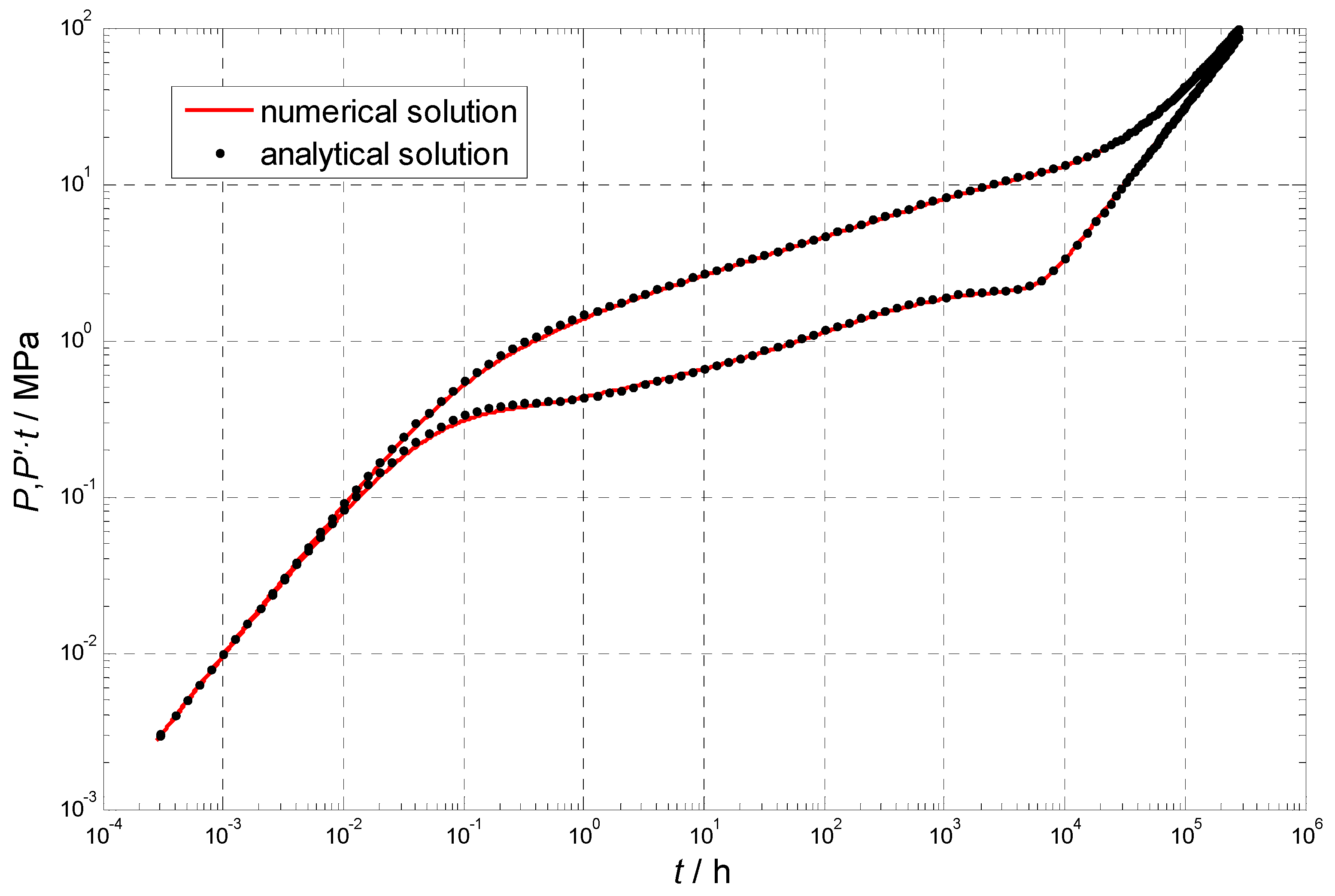
4.1. Accuracy Verification

To assess the precision of the aforementioned transient flow model, we simplify the fractured horizontal well into a fractured vertical configuration [37,40]. A reservoir radius of 500 m, a fracture half-length of 100 m, and a daily production rate of 20 cubic meters have been given, and the effects of TPG and stress sensitivity are disregarded. The numerical solution derived in this study is compared to an analytical solution, as presented in Figure 5. This comparison reveals a strong concordance between the two solutions, which indicates well the accuracy of the transient flow model.

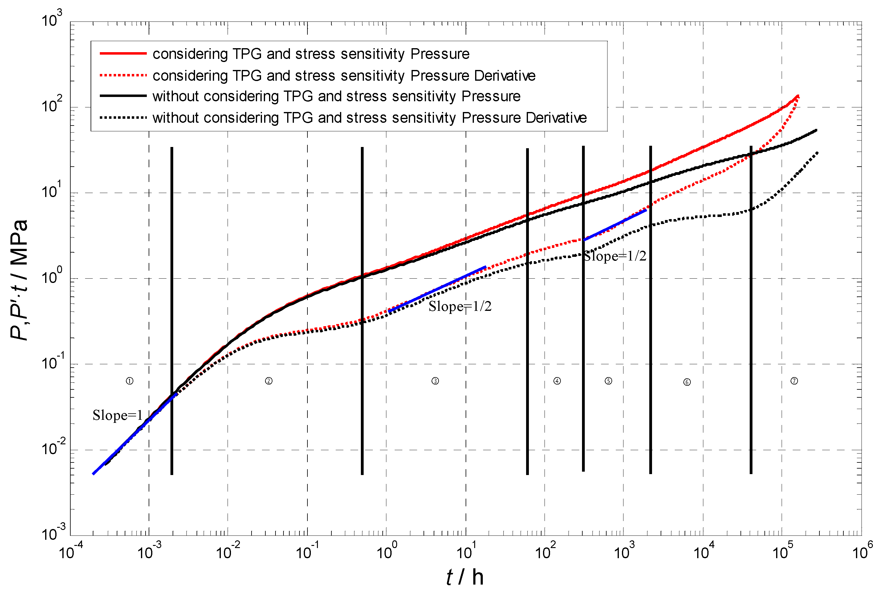
4.2. Flow Regime Analysis

In this paper, we analyze the flow regimes considering the effects of TPG and stress sensitivity, which can be categorized into seven distinct flow periods. Pressure-derivative curves are chosen to present the prominent characteristics of the different situations. The flow regimes are outlined in Figure 6 and described as follows:

(1)

Pure wellbore storage effect: This flow behavior occurs when the fluid has not yet penetrated into the wellbore. During this flow regime, the pressure and pressure-derivative curves completely overlap, displaying a unit slope line.

(2)

Channel flow: This situation represents the transitional flow regime between the pure wellbore storage effect and the fracture linear flow.

(3)

Fracture linear flow (Figure 7a): The fluid flows perpendicular to the fracture, resulting in a positive slope in the pressure-derivative curve. The main feature of this flow regime is that both the dimensionless pressure and the pressure-derivative curves are straight lines with a slope of 1/2.

(4)

Fracture radial flow (Figure 7b): When the fracture half-length is short and the spacing between fractures is wide, the fluid flows radially into each fracture before they begin to interact. This flow regime is characterized by a horizontal pressure-derivative curve. During this period, fluid flows radially from the fracture to the wellbore, and the main characteristic of this flow stage is a horizontal line on the dimensionless pressure-derivative curve.

(5)

Formation linear flow (Figure 7c): As the fractures begin to interact, the fluid flows parallel to the fractures, leading to a positive slope in the pressure-derivative curve. During this flow regime, the pressure-derivative curve shows a straight line with a slope of 1/2. This flow regime is mainly influenced by the dimensionless fracture conductivity and dimensionless fracture half-length.

(6)

Formation radial flow (Figure 7d): In this scenario, the reservoir is sufficiently large, and the production time is long enough, but the pressure wave has not yet reached the outer boundary; hence, the fluid flows radially into the fractured zone. This flow regime is also characterized by a horizontal pressure-derivative curve. During this flow regime, the dimensionless pressure-derivative curve shows a horizontal line but no longer adheres to the “0.5 slope line rule” when considering the TGP and the stress sensitivity.

(7)

Pseudo-steady flow: This regime emerges when the pressure wave reaches the closed outer boundary, resulting in a positive slope in the pressure-derivative curve. During this flow regime, the pressure and pressure-derivative curves still overlap but no longer adhere to the “unit slope line rule” when considering the TGP and the stress sensitivity.

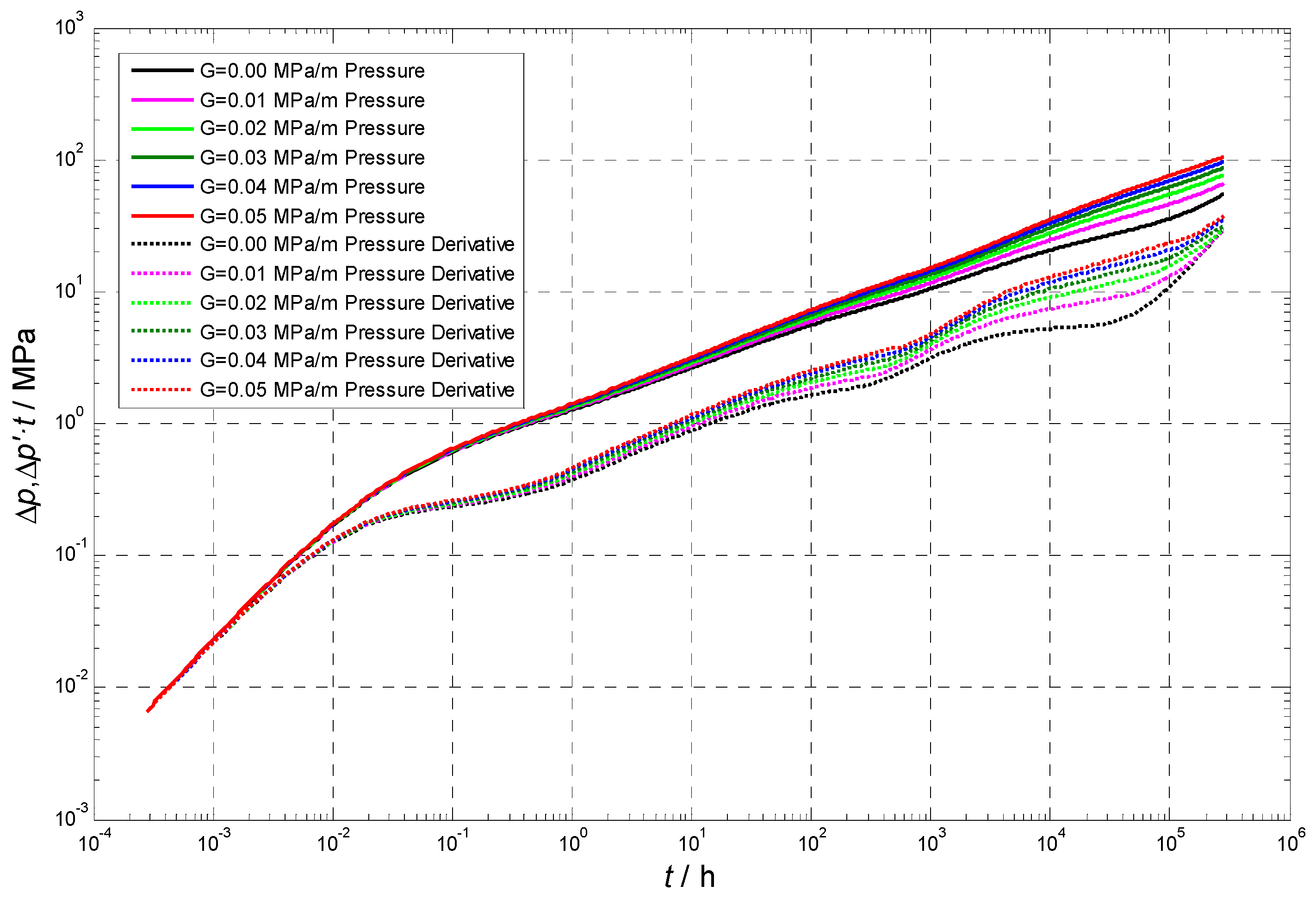
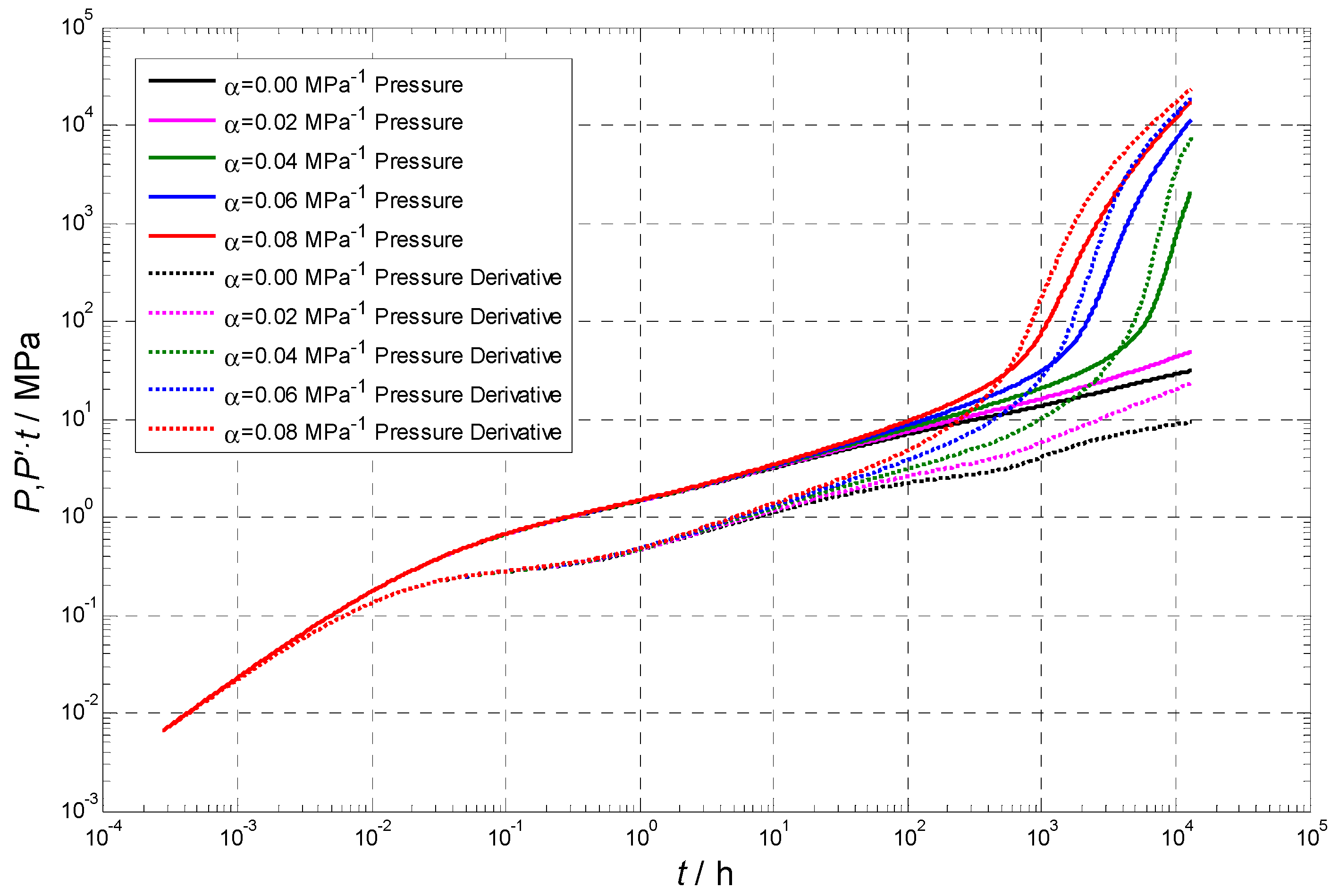
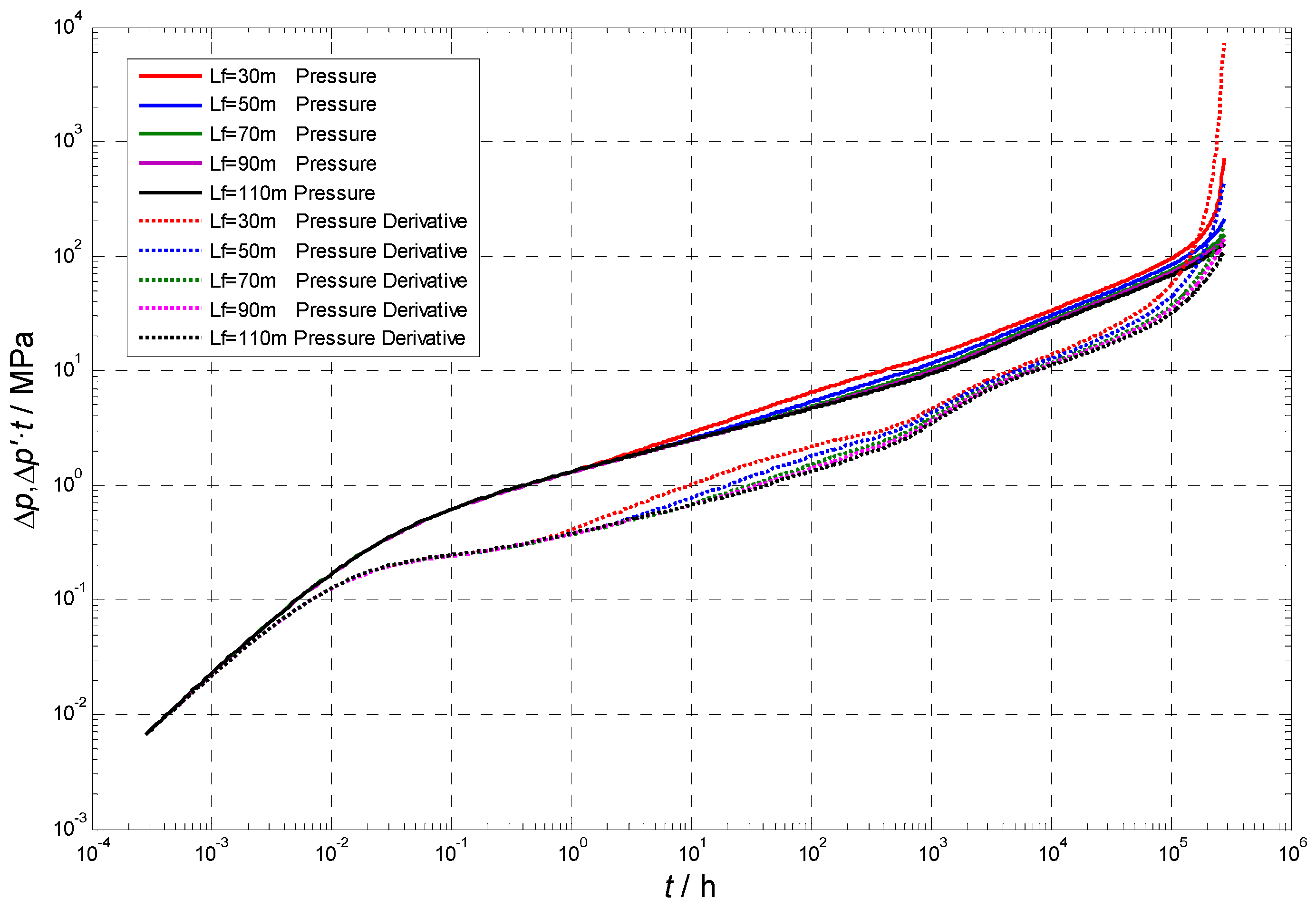
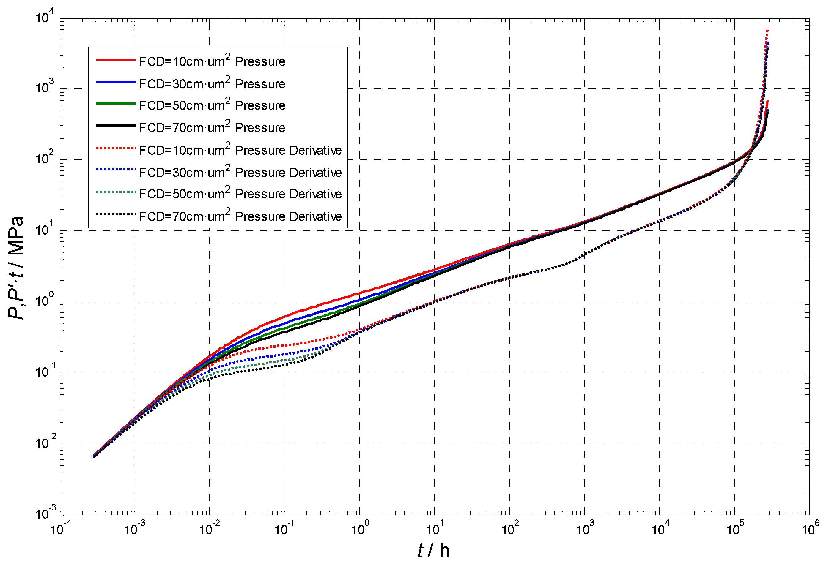
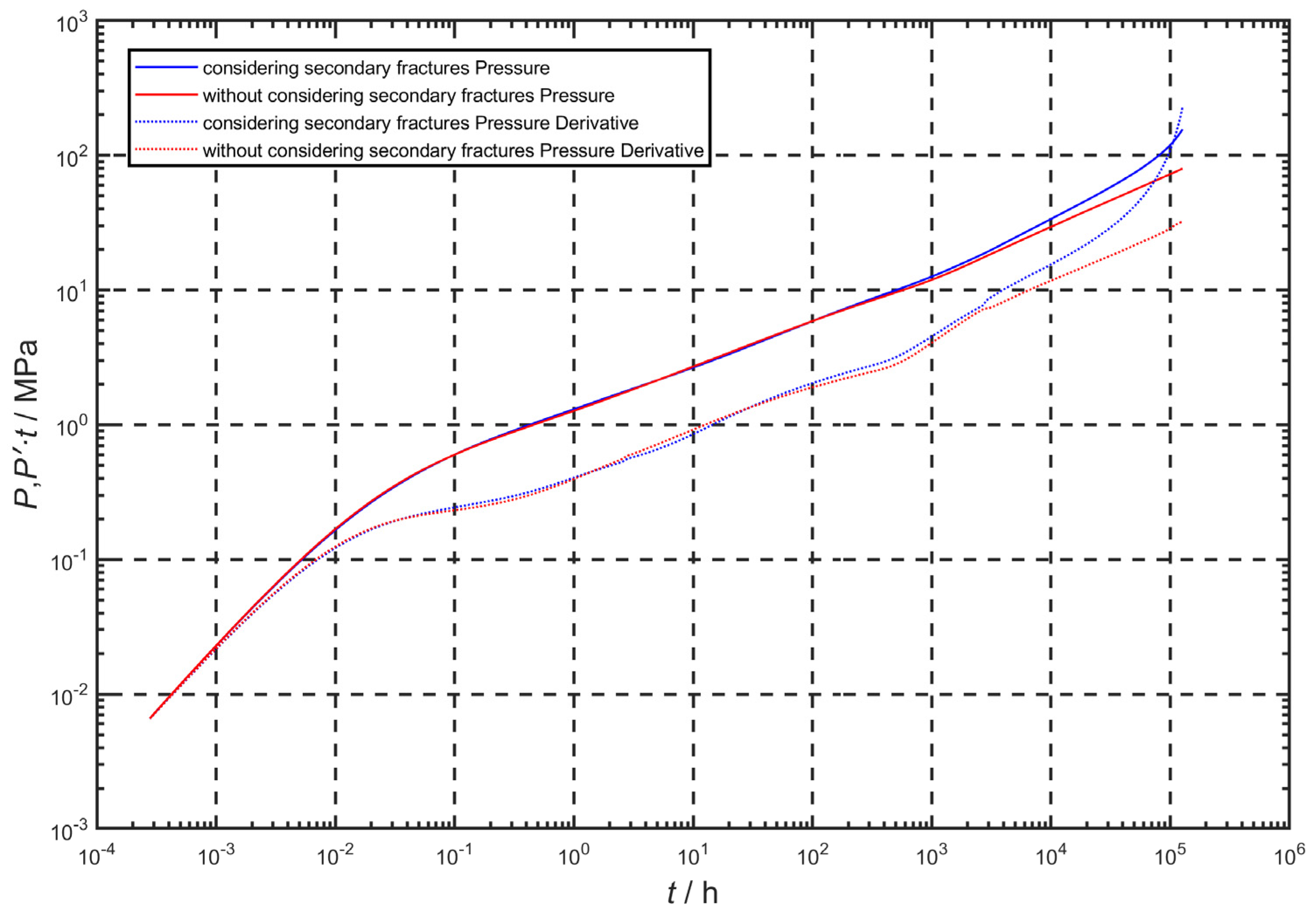
5. Sensitivity Analysis

Figure 8 demonstrates that the pressure-derivative curve exhibits an upward shift when the total pressure gradient (TPG) is considered and the stress sensitivity effects are neglected. This upward trend becomes more pronounced as the TPG increases, leading to increased difficulty in distinguishing between different flow regimes. Notably, the sensitivity of the pressure-derivative curve to TPG diminishes as the TPG value rises, but it increases over time.

Figure 9 illustrates that, as the permeability modulus increases, the pressure-derivative curve shifts upward. This upward trend becomes more prominent with higher permeability modulus values, particularly during later flow periods. The sensitivity of the pressure-derivative curve to the permeability modulus can be intensified over production time. Notably, as the permeability modulus increases, it becomes increasingly challenging to distinguish the fracture linear flow and the subsequent flow periods. Interestingly, when the permeability modulus remains constant, the upward shift initially intensifies but subsequently diminishes. This observation can be attributed to the exponential relationship between matrix permeability and pressure drop, which means that its variations become negligible, and the significance of the stress sensitivity effects can be reduced when matrix permeability decreases to a certain level.

Figure 10 demonstrates that, as the fracture half-length increases, the pressure-derivative curve exhibits a downward trend. The sensitivity of this curve to changes diminishes with the fracture half-length increasing. In addition, the fractur half-length primarily influences the fracture linear flow and subsequent flow periods, while the formation of fracture radial flow and the formation radial flow become increasingly challenging as the fracture half-length increases. Interestingly, during later flow periods, a decrease in the fracture half-length leads to a more severe upward shift in the pressure-derivative curve. This observation is attributed to the increasing influence of the matrix porous medium as the fracture half-length decreases, which enhances the effects of stress sensitivity.

Figure 11 illustrates that, as the fracture conductivity increases, the pressure-derivative curve exhibits a downward trend. The sensitivity of this curve to changes diminishes with fracture conductivity increasing. Notably, the fracture conductivity has a significant impact on the early flow period. In addition, a situation with an increase in fracture conductivity can be given to distinguish between various flow regimes, including transient flow, fracture linear flow, and fracture radial flow.

Figure 12 illustrates the effect of secondary fractures on formation pressure and pressure-derivative curve. In this case, two secondary fractures can be connected into each main crack, and the secondary fractures have a fracture half-length of 30 m [28], fracture conductivities (FCD) of 30 cm·μm² [37], and a fracture orientation of 45° to the main fracture. We can find that secondary fractures have a significant impact on the late flow period. Compared with the case without considering secondary fractures, the pressure-derivative curve of secondary fractures increases in the late flow period, which means that the pressure propagates faster to the boundary of the oil reservoir.

6. Conclusions

Drawing upon the discrete fracture model, this paper constructs a transient flow model specifically tailored to fractured horizontal wells in tight oil reservoirs. This model takes into account the intricate effects of total pressure gradient (TPG), stress sensitivity, fracture parameters, and fracture distribution. In addition, the finite-volume method is employed to solve this model. The precision of the aforementioned transient flow model is verified well with simplified numerical and analytical solutions. Finally, the sensitivity analysis of the obtained model has been discussed with such critical parameters. Some important conclusions have been summarized as follows.

As for fractured horizontal wells, there are typically seven distinct flow regimes, and the characteristic parameters for these have been given. However, incorporating the effects of TPG and stress sensitivity complicates the division of these flow regimes, because these factors contribute to an upward trend in the pressure-derivative curve. The pressure-derivative curve exhibits a more pronounced upward trend as the TPG and permeability modulus increase, which means that the pressure is more likely to reach the boundary as TPG increases. Notably, stress sensitivity primarily impacts the flow in later periods, and it initially enhances the upward trend but subsequently causes it to taper off, and its variations become negligible, and the significance of the stress sensitivity effects can be reduced when matrix permeability decreases to a certain level. Additionally, as the fracture half-length increases, the formation of fracture radial flow and formation radial flow becomes increasingly challenging because hydraulic fractures have a higher conductivity compared to the matrix and have an important role in pressure performance in tight oil development. Conversely, the fracture conductivity has a significant influence on the early flow period. Notably, accurately distinguishing flow regimes becomes more difficult with the increase in TPG and the permeability modulus, as well as the decrease in fracture conductivity. Compared with the case without considering secondary fractures, the pressure-derivative curve of secondary fractures increases in the late flow period, which means that the pressure propagates faster to the boundary of the oil reservoir.

In future works, the fracture network will be verified in the tight oil reservoir by microseism or fiber optic testing, and the discrete fracture model (DFM) or the embedded discrete fracture model (EDFM) will be employed to treat the fracture network when meaningful field data can be obtained [41,42]. In addition, after hydraulic fracturing, the fracturing liquid cannot flow back totally; hence, in the early flow period, the fluid flow should be a two-phase flow, which would affect the transient pressure performance in new models [43,44].

References

1. Qi, Y.; Zhang, T.; Chen, Q.; Ma, B.; Bai, J.; Ye, K.; Tang, J. What Low Frequency Distributed Acoustic Sensing Revealed of The Hydraulic Fracturing in Tight Oil Reservoir: Ordos Case Study. In Proceedings of the International Petroleum Technology Conference, Dhahran, Saudi Arabia, 18–20 February 2024. [Google Scholar]
2. Wang, H.; Zhou, W.; Wu, R.; Shang, Y.; Li, Z.; Li, G.; Huangfu, X.; Zhao, M.; Liu, X.; Wu, Y.; et al. Study on the Influence of DFN on Hydraulic Fracture Propagation for Horizontal Wells in Unconventional Resource—A Case Study from China. In Proceedings of the International Petroleum Technology Conference, Dhahran, Saudi Arabia, 18–20 February 2024. [Google Scholar]
3. Guo, G.; Evans, R.D. Pressure-transient behavior and inflow performance of horizontal wells intersecting discrete fractures. In Proceedings of the Offshore Technology Conference, Houston, TX, USA, 26–28 October 1993. SPE Paper 26446. [Google Scholar]
4. Guo, G.; Evans, R.D. Inflow performance and production forecasting of horizontal wells with multiple hydraulic fractures in low-permeability gas reservoirs. In Proceedings of the SPE Gas Technology Symposium, Calgary, AB, Canada, 28–30 June 1993. SPE Paper 26169. [Google Scholar]
5. Guo, G.; Evans, R.D. Inflow performance of a horizontal well intersecting natural fractures. In Proceedings of the OTC Arctic Technology Conference, Copenhagen, Denmark, 21–23 March 1993. SPE Paper 25501. [Google Scholar]
6. Guo, G.; Evans, R.D. Pressure-transient behavior for a horizontal well intersecting multiple random discrete fractures. In Proceedings of the SPE Annual Technical Conference and Exhibition, New Orleans, Louisiana, 25–28 September 1994. SPE Paper 28390. [Google Scholar]
7. Raghavan, R.S.; Chen, C.C.; Agarwal, B. An analysis of horizontal wells intercepted by multiple fractures. Soc. Pet. Eng. 1997, 2, 235–245. [Google Scholar] [CrossRef]
8. Zerzar, A.; Bettam, Y. Interpretation of Multiple Hydraulically Fractured Horizontal Wells in Closed Systems. In Proceedings of the SPE International Improved Oil Recovery Conference in Asia Pacific, Kuala Lumpur, Malaysia, 20–21 October 2003. SPE Paper 84888-MS. [Google Scholar]
9. Al-Kobaisi, M.; Ozkan, E.; Kazemi, H. A Hybrid Numerical-Analytical Model of Finite-Conductivity Vertical Fractures Intercepted by a Horizontal Well. In Proceedings of the SPE International Petroleum Conference in Mexico, Puebla Pue, Mexico, 7–9 November 2004. SPE Paper 92040-MS. [Google Scholar]
10. Wei, Y.; Economides, M.J. Transverse Hydraulic Fractures from a Horizontal Well. In Proceedings of the SPE Annual Technical Conference and Exhibition, Dallas, TX, USA, 9–12 October 2005. SPE Paper 94671-MS. [Google Scholar]
11. Medeiros, F.; Kurtoglu, B.; Ozkan, E.; Kazemi, H. Pressure-Transient Performances of Hydraulically Fractured Horizontal Wells in Locally and Globally Naturally Fractured Formations. In Proceedings of the International Petroleum Technology Conference, Dubai, United Arab Emirates, 4–6 December 2007. [Google Scholar]
12. Ozkan, E.; Brown, M.; Raghavan, R.; Kazemi, H. Comparison of fractured horizontal well performance in conventional and unconventional reservoirs. In Proceedings of the SPE Western Regional Meeting, San Jose, CA, USA, 24–26 March 2009. SPE Paper 121290-MS. [Google Scholar]
13. Yao, S.; Zeng, F.; Liu, H.; Zhao, G. A Semianalytical Model for Multistage Fractured Horizontal Wells. In Proceedings of the SPE Canadian Unconventional Resources Conference, Calgary, AB, Canada, 30 October–1 November 2012. SPE Paper 162784-MS. [Google Scholar]
14. Rbeawi, S.A.; Tiab, D. Transient pressure analysis of a horizontal well with multiple inclined hydraulic fractures using type-curve matching. In Proceedings of the SPE International Symposium and Exhibition on Formation Damage Control, Lafayette, LA, USA, 15–17 February 2012. SPE Paper 149902. [Google Scholar]
15. Zhao, Y.; Zhang, L.; Zhao, J.; Luo, J.; Zhang, B. “Triple porosity” modeling of transient well test and rate decline analysis for multi-fractured horizontal well in shale gas reservoirs. J. Pet. Sci. Eng. 2013, 110, 253–262. [Google Scholar] [CrossRef]
16. Yao, J.; Liu, P.; Wu, M. Well test analysis of fractured horizontal well in fractured reservoir. J. China Univ. Pet. 2013, 37, 107–113. [Google Scholar]
17. Fan, D.; Yao, J.; Sun, H.; Zeng, H.; Wang, W. A composite model of hydraulic fractured horizontal well with stimulated reservoir volume in tight oil & gas reservoir. J. Nat. Gas Sci. Eng. 2015, 24, 115–123. [Google Scholar]
18. Ren, Z.; Wang, X.; Han, G.; Liu, L.; Wang, X.; Zhang, G.; Lin, G.; Zhang, J.; Zhang, X. Transient pressure behavior of multi-stage fractured horizontal wells in stress-sensitive tight oil reservoirs. J. Pet. Sci. Eng. 2017, 157, 1197–1208. [Google Scholar]
19. Prada, A.; Civan, F. Modification of Darcy’s law for the threshold pressure gradient. J. Pet. Sci. Eng. 1999, 22, 237–240. [Google Scholar] [CrossRef]
20. Xiong, W.; Lei, Q.; Gao, S.; Hu, Z.; Xue, H. Pseudo threshold pressure gradient to flow for low permeability reservoirs. Pet. Explor. Dev. 2009, 36, 232–236. [Google Scholar]
21. Song, F.; Wang, J.; Liu, H. Static Threshold Pressure Gradient Characteristics of Liquid Influenced by Boundary Wettability. Chin. Phys. Lett. 2010, 27, 024704. [Google Scholar]
22. Zeng, B.; Cheng, L.; Li, C. Low velocity non-linear flow in ultra-low permeability reservoir. J. Pet. Sci. Eng. 2011, 80, 1–6. [Google Scholar] [CrossRef]
23. Zhu, W.; Song, H.; Huang, X.; Liu, X.; He, D.; Ran, Q. Pressure characteristics and effective deployment in a water-bearing tight gas reservoir with low-velocity non-Darcy flow. Energy Fuels 2011, 25, 1111–1117. [Google Scholar] [CrossRef]
24. Davies, J.P.; Davies, D.K. Stress-Dependent Permeability: Characterization and Modeling. In Proceedings of the SPE Annual Technical Conference and Exhibition, Houston, TX, USA, 3–6 October 1999. SPE Paper 56813-MS. [Google Scholar]
25. Shi, Y.; Sun, X. Stress sensitivity analysis of Changqing tight elastic reservoir. Pet. Explor. Dev. 2001, 28, 85–87. [Google Scholar]
26. Dautriat, J.; Gland, N.F.; Youssef, S.; Rosenberg, E.; Bekri, S. Stress-Dependent Permeabilities of Sandstones and Carbonates: Compression Experiments and Pore Network Modelings. In Proceedings of the SPE Annual Technical Conference and Exhibition, Anaheim, CA, USA, 11–14 November 2007. SPE Paper 110455-MS. [Google Scholar]
27. Diwu, P.; Liu, T.; You, Z.; Jiang, B.; Zhou, J. Effect of low velocity non-Darcy flow on pressure response in shale and tight oil reservoirs. Fuel 2018, 216, 398–406. [Google Scholar] [CrossRef]
28. Wu, Z.; Cui, C.; Lv, G.; Bing, S.; Cao, G. A multi-linear transient pressure model for multistage fractured horizontal well in tight oil reservoirs with considering threshold pressure gradient and stress sensitivity. J. Pet. Eng. 2019, 172, 839–854. [Google Scholar] [CrossRef]
29. Stress Fanchi, J.R.; Christiansen, R.L. Introduction to Petroleum Engineering; John Wiley & Sons: Hoboken, NJ, USA, 2016. [Google Scholar]
30. Karimi-Fard, M.; Durlofsky, L.J. An Efficient Discrete Fracture Model Applicable for General Purpose Reservoir Simulators. In Proceedings of the SPE Reservoir Simulation Symposium, Houston, TX, USA, 14–17 February 2003. SPE Paper 79699-MS. [Google Scholar]
31. Karimi-Fard, M.; Firoozabadi, A. Numerical Simulation of Water Injection in Fractured Media Using the Discrete-Fracture Model and the Galerkin Method. SPE Reserv. Eval. Eng. 2003, 6, 117–126. [Google Scholar] [CrossRef]
32. Hui, M.; Mallison, B.; Thomas, S.; Muron, P.; Rousset, M.; Earnest, E.; Playton, T.; Vo, H.; Jensen, C. A Hybrid Embedded Discrete Fracture Model and Dual-Porosity, Dual-Permeability Workflow for Hierarchical Treatment of Fractures in Practical Field Studies. SPE Res. Eval. Eng. 2023, 26, 888–904. [Google Scholar] [CrossRef]
33. Xiang, Y.; Wang, L.; Si, B.; Zhu, Y.; Yu, J.; Pan, Z. General Optimization Framework of Water Huff-n-Puff Based on Embedded Discrete Fracture Model Technology in Fractured Tight Oil Reservoir: A Case Study of Mazhong Reservoir in the Santanghu Basin in China. SPE J. 2023, 28, 3341–3357. [Google Scholar] [CrossRef]
34. Rashid, H.U.; Olufemi, O. A Continuous Projection-Based EDFM Model for Flow in Fractured Reservoirs. SPE J. 2024, 29, 476–492. [Google Scholar] [CrossRef]
35. Cinco-Ley, H.; Samaniego-V, F. Transient Pressure Analysis for Fractured Wells. J. Pet. Technol. 1981, 33, 1749–1766. [Google Scholar] [CrossRef]
36. Agarwal, R.G.; Carter, R.D.; Pollock, C.B. Evaluation and Performance Prediction of Low-Permeability Gas Wells Stimulated by Massive Hydraulic Fracturing. J. Pet. Technol. 1979, 31, 362–372. [Google Scholar] [CrossRef]
37. Feng, Q.; Xia, T.; Wang, S.; Singh, H. Pressure transient behavior of horizontal well with time-dependent fracture conductivity in tight oil reservoirs. Geofluids 2017, 2017, 5279792. [Google Scholar] [CrossRef]
38. Liu, Y.; Ding, Z.; He, F. Three kinds of methods for determining the start-up pressure gradients in low permeability reservoir. Well Test. 2002, 11, 1–4. [Google Scholar]
39. Liu, K.; Yin, D.; Sun, Y.; Xia, L. Analytical and experimental study of stress sensitivity effect on matrix/fracture transfer in fractured tight reservoir. J. Pet. Sci. Eng. 2020, 195, 107958. [Google Scholar] [CrossRef]
40. Kang, L.; Wang, G.; Zhang, X.; Guo, W.; Liang, B.; Jiang, P.; Liu, Y.; Gao, J.; Liu, D.; Yu, R.; et al. Dynamic Pressure Analysis of Shale Gas Wells Considering Three-Dimensional Distribution and Properties of the Hydraulic Fracture Network. Processes 2024, 12, 286. [Google Scholar] [CrossRef]
41. Liu, X.; Yan, J.; Lin, B.; Zhang, Q.; Wei, S. An integrated 3D fracture network reconstruction method based on microseismic events. J. Nat. Gas Sci. Eng. 2021, 95, 104182. [Google Scholar] [CrossRef]
42. Hou, B.; Zhang, Q.; Lv, J. Distributed Fiber Optic Monitoring of Asymmetric Fracture Swarm Propagation in Laminated Continental Shale Oil Reservoirs. Rock Mech. Rock Eng. 2024, 1–21. [Google Scholar] [CrossRef]
43. Dahi Taleghani, A.; Cai, Y.; Pouya, A. Fracture closure modes during flowback from hydraulic fractures. Int. J. Numer. Anal. Methods Geomech. 2020, 44, 1695–1704. [Google Scholar] [CrossRef]
44. Jia, P.; Cheng, L.; Huang, S.; Xue, Y.; Clarkson, C.R.; Williams-Kovacs, J.D.; Wang, S.; Wang, D. Dynamic coupling of analytical linear flow solution and numerical fracture model for simulating early-time flowback of fractured tight oil wells (planar fracture and complex fracture network). J. Pet. Sci. Eng. 2019, 177, 1–23. [Google Scholar] [CrossRef]
Figure 1. The schematic of a fractured horizontal well in tight oil reservoirs.
Energies 17 02556 g001
Figure 2. The schematic figure of the discrete fracture model. (a) single-porosity model; (b) discrete fracture model.
Energies 17 02556 g002
Figure 3. The schematic of the cell vertex network model. (a) control volume cells of the matrix; (b) control volume cells contain fracture.
Energies 17 02556 g003
Figure 4. The schematic of transmission between neighbored grids.
Energies 17 02556 g004
Figure 5. Comparison between numerical solution and analytical solution.
Energies 17 02556 g005
Figure 6. Pressure performance behavior of fracturing horizontal wells in tight oil reservoirs.
Energies 17 02556 g006
Figure 7. The schematics of the main flow regimes of a fractured horizontal well. (a) fracture linear flow; (b) fracture radial flow; (c) formation linear flow; (d) formation radial flow.
Energies 17 02556 g007
Figure 8. Effect of TPG on formation pressure and pressure-derivative curve.
Energies 17 02556 g008
Figure 9. Effect of permeability modulus on formation pressure and pressure-derivative curve.
Energies 17 02556 g009
Figure 10. Effect of the fracture half-length on formation pressure and pressure-derivative curve.
Energies 17 02556 g010
Figure 11. Effect of fracture conductivity on formation pressure and pressure-derivative curve.
Energies 17 02556 g011
Figure 12. Effect of secondary fractures on formation pressure and pressure-derivative curve.
Energies 17 02556 g012
Disclaimer/Publisher’s Note: The statements, opinions and data contained in all publications are solely those of the individual author(s) and contributor(s) and not of MDPI and/or the editor(s). MDPI and/or the editor(s) disclaim responsibility for any injury to people or property resulting from any ideas, methods, instructions or products referred to in the content.