End-to-End Top-Down Load Forecasting Model for Residential Consumers

Abstract

This study presents an efficient end-to-end (E2E) learning approach for the short-term load forecasting of hierarchically structured residential consumers based on the principles of a top-down (TD) approach. This technique employs a neural network for predicting load at lower hierarchical levels based on the aggregated one at the top. A simulation is carried out with 9 (from 2013 to 2021) years of energy consumption data of 50 houses located in the United States of America. Simulation results demonstrate that the E2E model, which uses a single model for different nodes and is based on the principles of a top-down approach, shows huge potential for improving forecasting accuracy, making it a valuable tool for grid planners. Model inputs are derived from the aggregated residential category and the specific cluster targeted for forecasting. The proposed model can accurately forecast any residential consumption cluster without requiring any hyperparameter adjustments. According to the experimental analysis, the E2E model outperformed a two-stage methodology and a benchmarked Seasonal Autoregressive Integrated Moving Average (SARIMA) and Support Vector Regression (SVR) model by a mean absolute percentage error (MAPE) of 2.27%.

1. Introduction

A load forecast is one of the vital phases for planning in the electricity sector. An accurate load forecast model helps power system operators make informed decisions, such as scheduled maintenance, economic dispatch, and unit commitment [1]. Particularly, short-term hourly forecasts are vital in the efficacy of day-ahead markets [2]. Traditionally, many models based on regression, such as Autoregressive Integrated Moving Average ARIMA), Support Vector Regression (SVR), and exponential regression are used to forecast load consumption [3,4]. However, the integration of Distributed Energy Resources (DERs) and interruptible loads has altered the consumption profile, making it difficult for the existing regression-based models to forecast load accurately. While these models are proficient with linear loads, the increasing prevalence of Electric Vehicles (EVs), energy storage systems (ESS), and renewable energy sources (RESs) has altered the load profile from linear to nonlinear, which significantly impacts low-voltage networks. Consequently, it becomes crucial to direct attention toward low-voltage consumers, particularly in the residential sector. Accurate residential load forecasting can unlock opportunities for the demand response for which residential customers are the primary targets. However, the inherent volatility in their consumption patterns presents a significant challenge for accurate forecasting.

The existing literature on residential consumers predominantly concentrates on constructing precise forecast models tailored to individual households [5,6,7]. However, due to the unpredictable nature of consumption behavior, it becomes a challenge for a single model to accurately predict the load of different households. While certain models exist to forecast load for multiple individual households, these are typically designed to estimate daily consumption rather than hourly intervals. Alternatively, some models in the literature aim to forecast the hourly consumption of aggregated groups of houses [8,9]. However, such methodologies often rely on intricate details about individual homes, including appliance-level data. In a nutshell, most existing models primarily focus on predicting energy usage for either single residences or clusters of homes, with their efficacy often hinging on extensive data regarding energy-usage patterns. For instance, in a recent study by Hadar et al. in [10], a model based on Long Short-Term Memory (LSTM) was developed to forecast the combined consumption of selected houses. Despite being rigorously tested across various datasets to ascertain its accuracy; this model forecasts load as an aggregate sum of all the included households and disregards the individual forecasts. Moreover, the fluctuating consumption patterns observed in households make it impractical for a single model to provide accurate forecasts for all residential consumers involved. Another group of authors Zheng et al. [11] directed their efforts toward devising a model capable of providing both point and probability forecasts for residential households. The forecast model for the residential sector heavily relies on private household data, which is a huge challenge, but the widespread adoption of smart meters has facilitated access to time-series consumption data from these residences. Consequently, there is a growing need to develop forecast models that rely on historical time-series data rather than relying on personal resident details.

The residential sector encompasses a diverse array of consumers, each distinguished by various factors, including demographics, socio-economic status, lifestyle, and consumption patterns [12]. Instead of treating all residential consumers as a homogeneous group, it is more appropriate to leverage time-series data collected from smart meters and focus on hierarchical load forecasting. This approach enables a deeper understanding of the distinct consumer groups within the sector and facilitates the identification of those most suitable for implementing energy conservation and demand-side management strategies. Additionally, accurate forecasts for the different consumer groups are essential for grid operators in planning their demand and forecasting needs. Hierarchical load forecasts offer a means to achieve this, ensuring comprehensive forecasting across all groups within the residential sector.

There are three main types of approaches for hierarchical load forecasting: top-down (TD), bottom-up (BU), and middle-out approaches [13,14]. In the TD approach, the forecast is performed at the highest level of the hierarchy, which is then distributed to lower levels, whereas in the BU approach, the forecast is performed at a lower level of the hierarchy, which is then summed up to the aggregated level. The middle-out approach, as explained in [14], combines the benefits of both the TD and BU approaches by selecting a middle level in the hierarchy and generating forecasts for it. For the higher levels, the forecasts at the middle level are summed up to obtain higher-level forecasts. While many current models adopt a bottom-up approach to forecasting, this method necessitates multiple forecasting models and intricate data inputs at lower hierarchical levels. This approach holds promise for precise forecasting at lower hierarchy levels, but errors tend to escalate when attempting to forecast at higher levels of hierarchy. On the other hand, the TD approach, while simpler, may result in reduced accuracy at other hierarchy levels due to its dependence on distribution ratios for dividing forecasts at lower levels [13]. The increase in error occurs when the unique characteristics of lower levels are not considered. A residential sector organized in a hierarchical structure will also require the design of numerous independent forecast models for each group under the BU approach where each model requires detailed input features explaining the inherent characteristics of the group—a laborious task from a practical implementation standpoint. Nonetheless, the concept behind the TD approach is appealing because it offers simpler implementation.

In this paper, we introduce a novel end-to-end learning model driven by the concept of a top-down hierarchical load-forecasting approach. This model leverages smart meter data to its fullest extent, prioritizing essential input features while minimizing reliance on exogenous input features for performance. In summary, our primary contributions in this paper include the following:

• The development of a high-performing end-to-end (E2E) learning model for residential sector forecasting, drawing from the core idea of the top-down approach.
• The model’s capability to forecast the load of various subgroups within a hierarchy without requiring hyperparameter tuning.
• The model’s ability to facilitate cross-learning across different hierarchy levels to enhance forecasting accuracy.

The rest of the paper is organized as follows. The related work is summarized in Section 2. Section 3 presents the proposed methodology and describes its main components. The forecasting results are presented in Section 4, along with a comparison with other forecasting models. Finally, the paper added concluding remarks in Section 5.

2. Related Work

In preceding years, numerous models for forecasting electricity demand have leaned on methods, such as ARIMA, Seasonal Autoregressive Integrated Moving Average (SARIMA), and SARIMAX (SARIMA with exogenous variables) [15,16]. These models, designed for time-dependent data, are particularly effective in predicting electricity demand in scenarios where the required forecasting series is linear in nature. For example, Lu et al. in [17] present a short-term load-forecasting approach centered on load decomposition and numerical weather prediction, which they have tested on a city grid in South China. In this method, the load is divided into two distinct components: the base component and the weather-sensitive component, with each being forecasted independently. For the time-series forecasting of the base component, the Holt–Winters model is applied. Additionally, the SVR model is trained using historical load data and meteorological information to predict the weather-sensitive component. However, the residential time-series data typically lack linearity due to the presence of diverse non-linear loads, such as EVs, rooftop photovoltaic (PV) systems, or simply due to differences in demographics.

Numerous researchers have dedicated efforts to developing precise forecast models within the power sector, primarily concentrating on predicting demand at the utility scale [18,19]. For example, Tindra et al., in their work in [18], specifically created a peak load-forecast model tailored for Banda Aceh City to address the escalating need for electrical energy. This model, leveraging the Adaptive Neuro-Fuzzy Inference System, incorporates variables, such as the temperature, humidity, and electrical load during peak hours. Shohan et al. [20] devise a hybrid approach employing LSTM techniques and a neural prophet via an artificial neural network (ANN) to forecast load one hour and one day ahead at the utility scale. Al-ani et al. [21] undertook load forecasting at the transmission level utilizing smart meter data, employing a forecast model rooted in ANN and Fuzzy logic. The influence of seasonal variations has not been included in this model. Models using techniques, such as SARIMA, can capture seasonality in the data. However, it is hard to capture the exact seasonal time. Therefore, Musbah and El-Hawary developed a SARIMA model in which the hourly electrical load data are transformed into the frequency domain to detect the existence of seasonal components from the time-series electrical load [22]. While these models demonstrate commendable accuracy, their primary focus lies within the broader domains of the power sector, encompassing the utility scale and transmission levels, with limited attention given to one of the most challenging sectors within utilities, namely the residential sector. Furthermore, in recent years, there has been the increasing adoption of renewable energy sources within the residential sector. Hence, the residential sector encompasses both consumers and prosumers [23]. The effective management of this intricate electricity network, integrating variable generators, is paramount. Improved forecast models are key, as the precise prediction of residential electricity usage is essential for optimizing overall energy efficiency in the system. In the residential sector, simply having forecasts for individual houses or different aggregation groups of houses is insufficient. It is more valuable to gain a comprehensive understanding of how forecasts appear across the residential hierarchy.

Many studies have been dedicated to building forecast models for hierarchical load structures [24,25,26]. The hierarchical forecast model follows either a TD or BU approach. In BU, forecasts are conducted at lower levels of the hierarchy, which are summed up to obtain an estimate at a higher level. Therefore, the BU approach necessitates employing several forecast models, each corresponding to a sub-level within the hierarchy, and necessitates the need for optimizing each model to achieve the most accurate estimation, whereas in the TD approach, the forecast is performed at the highest level of the hierarchy, which is then distributed down to lower levels using mathematical relationships between different levels of the hierarchy [26]. The TD approach provides better accuracy at the aggregated level but may lead to lower accuracy at lower levels due to the possibility of the loss of information. Additionally, the TD approach is straightforward to implement.

Most of the presented hierarchical forecasting models adopt the BU approach because it offers superior accuracy at the lower levels of the hierarchy. However, this accuracy hinges on the substantial volume of input data required. For example, Wang et al., in [27], propose a BU approach to forecast the load of a house using load characteristics of the appliances. Whereas Farzan et al., in [28], propose a BU engineering model to simulate the electricity demand of households and communities, where Markov chain, Bayesian, and logistic techniques are used to model the occupancy behavior along with the adoption of other technologies. Besides, the BU approach is not the best choice for aggregated-level forecasts as the errors at the lower level get compounded at the higher level. Another challenge encountered in the BU approach is that of coherence, where forecasts at lower levels are not appropriately aggregated to higher levels [29]. Hence, a considerable body of literature is dedicated to enhancing forecasting coherence across various hierarchy levels. The study conducted in [29] addresses this issue by focusing on forecasting the load of a distribution transformer hierarchy, which includes single-phase customers, the load at each phase, and the total load across all phases. In this study, base models utilizing ARIMA are employed to forecast at each hierarchical level. Subsequently, a distinct model based on minimum trace (MinT) is trained to effectively reconcile the base forecasts, thereby enhancing overall accuracy. Given the intricacies within the energy sector, utilizing the BU approach for forecasting is increasingly challenging in practical scenarios. Conversely, the TD approach provides a simpler implementation process. Leveraging its core principles in model design could lead to precise forecasts, while its simplicity holds promise for practical applications.

Rivera-Caballero et al., in [30], developed a model utilizing Multilayer Perceptron (MLP) and LSTM architectures to forecast the load demand of a substation comprising three feeders arranged hierarchically. They conducted a comparative analysis of accuracy between two scenarios: one considering the hierarchical structure and the other without it. The results demonstrated that the hierarchical load-forecast model outperforms individual forecasts in terms of accuracy. However, this paper primarily focuses on using the BU approach for forecasting at higher hierarchy levels with the methodology designed for the feeder-level consumption, which is not as volatile as the residential group.

In addition, it is widely recognized that the non-linear loads at the consumer level have altered the load profile [31,32,33]. As a result, it becomes imperative to gain a comprehensive understanding of the unique load profiles that the grid needs to accommodate. Rhodes et al. focused on identifying the distinct load profiles for residential consumers in the winter and summer seasons [34]. An analysis of load profiles is useful in identifying consumers who may benefit the most from energy conservation and time-of-use policies. Quilumba et al., in [24], classified the households with similar consumption patterns into one cluster and built a separate forecast model for each cluster. Although this approach could forecast load consumption for the entire residential group, it is computationally extensive due to the requirement for multiple forecast models. In contrast, Angizeh et al. combined the TD and BU approaches to estimate regional-level consumption [35]. This approach employs a simulator based on the physical characteristics of the building to model the consumption of each sector. However, this model is suitable for areas or cases where fine granular data are unavailable. A comparison between the performance of the BU and TD models was conducted in [36], and the BU approach was found to be better than TD in terms of accuracy at the lower levels of hierarchy. However, the forecast is for the total annual load consumption rather than the hourly load forecast. However, the availability of high-resolution data from smart meters, combined with the pattern recognition capabilities of neural networks, presents an opportunity to employ the TD approach without compromising accuracy across the entire hierarchy.

In [37], a global model is introduced for predicting load across an entire hierarchy. This methodology is assessed using a distribution network comprising various aggregation levels, encompassing individual consumers, feeders, and transformer substations within the hierarchy. Unlike conventional hierarchical methods, which entail multiple forecast models for each load series within the hierarchy, the proposed approach involves stacking samples from all load series within the hierarchy and subsequently fitting a single univariate forecasting function to the entire stacked dataset. The global model, utilizing the N-BEATS architecture, incorporates historical lags and calendar variables as input. The authors’ proposed approach entails supplementary steps aimed at enhancing the global model’s performance. This includes generating additional forecasts at various clusters, followed by an optimal ensemble step that combines all forecasts. While this global model effectively addresses the entirety of the hierarchy, it necessitates supplementary steps for optimizing forecasting accuracy. The findings illustrate the mean absolute percentage error (MAPE) in the range of 8.1–8.3% and mean absolute scaled error (MASE) values ranging between 0.6 and 0.8, which remains substantial compared to a simplistic naive approach yielding an MASE of 1.

Thus, there has not been significant research focusing on accurately estimating the load consumption for the entire residential group, including the different sub-groups with minimal exogenous data. Consequently, this study centers on constructing a hierarchical forecasting model with an E2E learning approach based on the concepts of the TD approach. The model relies solely on input features derived from smart meter data, making it a more practical and efficient for implementation because it does not depend on exogenous variables.

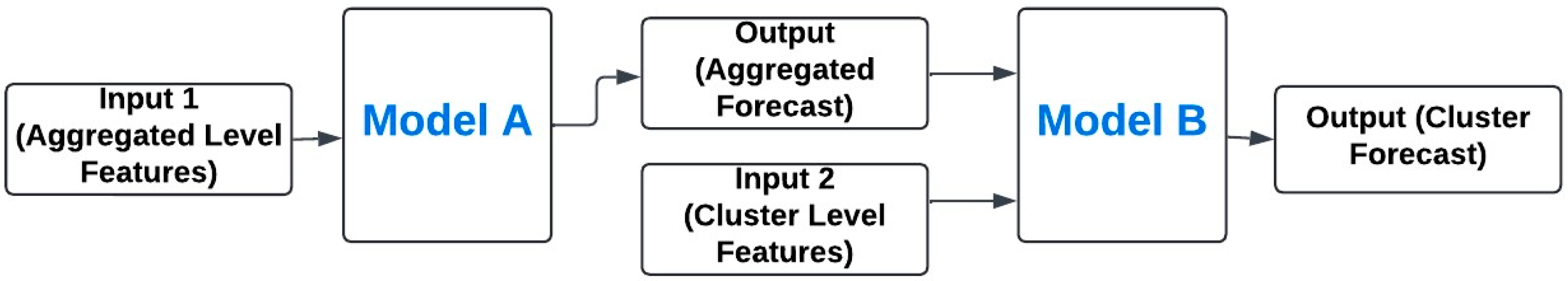
In one of our previous works [26], we tested the efficacy of models based on the TD approach by building a two-stage model to forecast the load consumption of the residential hierarchical structure. It consists of two models, where model A uses features of the aggregated level and is trained to forecast load at the aggregated level. On the other hand, model B uses two categories of features: the output of model A and specific features of the cluster for which the forecast is required. Each of these models is based on a neural network and requires independent sequential training of the two models. In comparison with the traditionally used SARIMA and SVR forecast model, this methodology performs better and shows significant potential in employing the concepts of the TD approach. However, it still requires the training of two separate models adding to the computation time. Moreover, the input features for the two models are dependent on the individual features of the aggregated level of hierarchy and the level for which the forecast is required, thereby disregarding the relationship between the two levels of the hierarchy i.e., the aggregated level and the cluster for which the forecast is required. This paper builds upon the work presented in [26] and introduces a single model capable of predicting load consumption at all levels of the hierarchy. Furthermore, it incorporates distinctive features that explain the relationship between the aggregated level and the cluster, thereby promoting cross-learning between different levels of the hierarchy. Therefore, this approach has a significant contribution to enhancing forecasting accuracy.

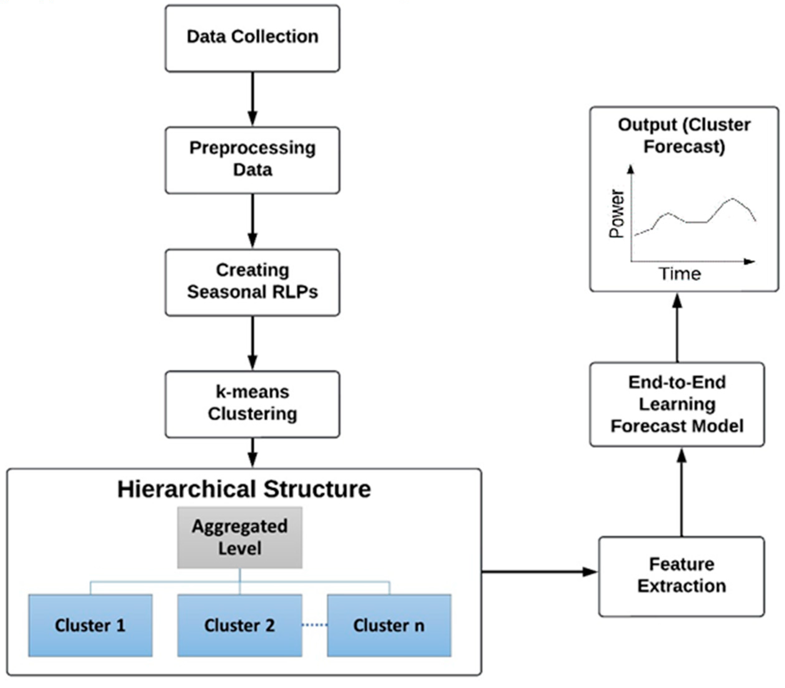
An E2E learning model is a system where the model learns all the steps from input to output simultaneously [38]. One of its widely used applications is for autonomous driving. In [39], Chen and Huang introduce an E2E learning model designed to predict the steering angle of a car using raw images as input. In this E2E approach, all the intermediate steps, such as lane detection, path planning, and steering control, are avoided. Motivated by this application, our paper aims to develop an E2E learning model centered on the TD hierarchical forecasting concept. This model predicts residential consumer load consumption within the power sector by incorporating features from different hierarchical levels simultaneously and training the model accordingly. In traditional TD approaches, forecasting occurs at the highest hierarchy level, and predictions are subsequently distributed to lower levels using historical mathematical distribution ratios. Similarly, our model adopts this principle by leveraging aggregated-level features alongside those specific to the lower levels where forecasting is necessary. This E2E learning model integrates the notion of cross-learning from features to enhance forecasting accuracy. As a result, the proposed methodology facilitates load-consumption forecasting across all hierarchical nodes.

3. Methodology

The proposed methodology is based on two main building blocks: building hierarchy following clustering and the end-to-end learning forecast model. Figure 1 illustrates the proposed framework for estimating the load of residential consumers.

3.1. Building Hierarchical Structure

The hierarchical structure is created as the first stage in the proposed methodology. The power sector’s inherent hierarchical structure serves as the motivation for the hierarchy building concept. In addition, a residential hierarchical structure facilitates the identification of groups that are present within this sector. Various methods exist for this purpose as some approaches group houses based on their geographical location, while some rely on similarities in consumption patterns. Leveraging smart meter data, this work constructs the hierarchy using the daily load profiles of individual consumers. The daily load profiles are used to create seasonal representative load profiles (RLPs). There are different methods to create seasonal RLPs. The first method involves two-stage clustering, where each customer is individually clustered based on their daily load profiles. The cluster with the highest number of load profiles becomes the representative cluster for that customer, and the average load profile within that cluster is used as the RLP. The second method calculates the RLP by averaging the daily load profiles of each customer and normalizing it relative to their maximum power value. Both of these methods were evaluated in [26], and it was found that the average method gives better RLPs. This work builds upon those findings, and seasonal RLPs are created for each customer for all four seasons: winter, summer, fall, and spring. These seasonal RLPs are used as input features for clustering algorithms, which are used to create hierarchical structures. Several algorithms are available in the literature for clustering. In a previous investigation [26], four clustering algorithms were evaluated for their effectiveness in creating high-quality clusters. Among those, the K-means clustering algorithm demonstrated superior performance in this context. Building upon prior research, this work employs the K-means clustering algorithm, where the seasonal RLPs serve as input to the clustering process. The clustering process employs time-series K-means clustering with dynamic time warping (DTW) as the metric. As a result, the algorithm groups households with similar load profiles into the same cluster. The elbow method [40,41] is utilized to determine the optimal number of clusters. In the elbow method, the K-means clustering algorithm is applied across a range of K values. For each K value, the sum of squared distances of data points to their respective cluster centroids, known as the within-cluster sum of squares (WCSS), is calculated [41]. A curve is then plotted for the values of K against their corresponding WCSS. The optimal value of K is chosen as the point on the curve where the WCSS drops significantly, resembling an elbow. Once clustering is complete, a hierarchical structure of households is established with the lowest level corresponding to individual houses with each cluster. Moving up a level, we encounter a cluster of households. Finally, the highest level represents the aggregated sum of all clusters. The hierarchical forecast in this work is limited to the cluster level and the aggregated level. The forecast model is not designed to forecast load consumption for individual load series of each house, as the fluctuating consumption patterns of households make it almost impossible for a single model to give accurate forecasting results for all the individual time series of each household.

3.2. End-to-End Learning Model

The proposed forecasting model is built on the top-down hierarchical approach. As explained in the TD approach, the forecast is performed at the highest level of the hierarchy, which is then distributed to the lower levels using mathematical distribution ratios. In this case, no consideration is given to the distinct input features of the cluster for which the forecast is required. Besides, it does not even consider the relationship between the aggregated and lower levels of the hierarchy. Traditionally, the mathematical ratios are either the average of historical proportions or the proportion of the historical average. The use of these ratios is beneficial in cases where the forecasting is required at a higher level of aggregation, such as monthly peak or total daily consumption, weekly sales, and so on. This approach is not suitable for forecasting hourly load consumption. On the other hand, the bottom-up approach requires an individually designed forecast model for each cluster group involved in the hierarchy, which basically means having multiple models, each having a probable different architecture and model type.

By considering the limitations discussed above, the proposed methodology incorporates the TD principles but also includes a cross-learning approach. This means that this paper designs a single E2E model by making use of input features derived from both aggregated and cluster levels along with an additional important feature, which explains the relationship between the different hierarchical levels. This approach is easier from an implementation perspective and combines the advantages of a top-down approach and incorporates cross-learning features.

An E2E model is designed for the entire hierarchy to forecast load at any node by giving input features of the aggregated level and of the relevant node. The input features to the model are based on the historical consumption data and calendar variables, further elaborated in

Table 1. Input features for the hierarchy.

Level	Input Features	Description
Aggregated Level	Lavg_3h, Lavg_t_d	Average of load consumption in the previous 3 h and average load consumption of the same 2 days of the week at the same time
	Lt−24, Lt_d, Lt−1, Lt−2, Lt−3, Lt−21, Lt−22, Lt−23, Lt−24	Load consumption at the same time as the previous day, load consumption on the same day of the week at the same time
	LTF1, LTF2, LTF3, LTF4, LTF5	Load tracking features as explained in Equations (1)–(5)
Cluster Level	Lc,avg_t_d	Average load consumption of the whole day
	Lc,t−24, Lc,t−1	Load consumption at the same time as the previous day and previous hour
	Rc	Ratio between aggregated and cluster-level consumption
Calendar features	hsine, hcos, dsine, dcos, msine, mcos, H	Hour of the day, day of the week, and month of the year expressed as the cyclic feature

.

The input features at the aggregated level consist of lag features, an average of the previous hour consumption, and load tracking features [42]. In time-series data, the load consumption at any hour does not depend only on the absolute value of historical consumption but also on how the consumption changes with time; therefore, a special group of features known as load tracking features (LTFs) is introduced in the model elaborated in [42]. These features are useful in describing the rate of change to the model. The LTFs depend on the hourly and daily load change, as shown in Equations (1)–(5), where $\mathrm{DLC}\mathrm{and}\mathrm{HLC}$ represent the daily load change and hourly load change, respectively, with subscript $\mathrm{D}$ and $\mathrm{H}$ representing the forecasting day and forecasting hour. For example, L_D,H denotes the load during the current hour of the forecasted day.

$${\mathrm{LTF}}_1={\mathrm{L}}_{\mathrm{D},\mathrm{H}-1}+{\mathrm{DLC}}_{\mathrm{D}-1,\mathrm{H}}$$

(1)

$${\mathrm{LTF}}_2={\mathrm{L}}_{\mathrm{D}-1,\mathrm{H}}+{\mathrm{HLC}}_{\mathrm{D}-1,\mathrm{H}}$$

(2)

$${\mathrm{LTF}}_3={\mathrm{L}}_{\mathrm{D},\mathrm{H}-1}+\mathrm{mean}({\mathrm{HLC}}_{\mathrm{D}-1,\mathrm{H}}+{\mathrm{HLC}}_{\mathrm{D}-2,\mathrm{H}})$$

(3)

$${\mathrm{LTF}}_4={\mathrm{L}}_{\mathrm{D},\mathrm{H}-1}+{\mathrm{HLC}}_{\mathrm{D}-7,\mathrm{H}}$$

(4)

$${\mathrm{LTF}}_5={\mathrm{L}}_{\mathrm{D},\mathrm{H}-1}+\mathrm{mean}({\mathrm{HLC}}_{\mathrm{D}-1,\mathrm{H}}+{\mathrm{HLC}}_{\mathrm{D}-7,\mathrm{H}})$$

(5)

The cluster features include the average of previous hours, lag features, and the ratio representing the relationship between the aggregated and cluster-level consumption. In addition to that, calendar variables, such as hour of the day, day of the month, and month are included as cyclic features. All the features are derived from historical consumption only and have not considered any exogenous features. Several features can be extracted from historical load data; however, to reduce the problem of dimensionality, most optimal input features are selected using the statistical Spearman coefficient [12,43].

The architecture of the proposed methodology, including the E2E learning model, is demonstrated in Figure 2. The E2E learning model relies on a single feedforward neural network architecture enhanced with dropout regularization. This model is designed to accommodate both cluster-level and aggregated-level forecasting tasks based on the specific requirements of the application. There are three sources of input features, i.e., aggregated, cluster level, and calendar variables, which are concatenated by the model before being processed by the hidden dense layers. The first hidden layer is a dense layer having 100 neurons, followed by a dropout layer. The incorporation of dropout regularization helps to prevent overfitting and improves the model’s generalization capabilities, ensuring robust performance across different datasets and scenarios. The activation function used is a rectified linear unit. The hyperparameters are tuned in to give the best possible forecasting accuracy. The model is compiled using Adam optimizer with the mean squared error as a loss function.

In our prior research [26], a two-stage methodology was assessed for forecasting load consumption within the residential hierarchy. This approach, comparable to the TD method, comprises two neural models trained separately. The first model, labeled as model A, is trained to predict load consumption at the aggregated level using only aggregated-level input features. Meanwhile, model B is tasked with forecasting load consumption at the cluster level, utilizing both its distinct features and the output of Model A. Illustrated in Figure 3 is a block diagram depicting the previously proposed two-stage model approach, showcasing the two neural network-based models. This methodology entailed training two models independently for each cluster forecast, and when compared to the BU approach, the methodology exhibited reduced error. The outcomes of the two-stage model approach demonstrated considerable potential in enhancing forecasting accuracy through the TD method, but the model in [26] did not consider any cross-learning features. Besides, the necessity of training two distinct models prompted the development of an end-to-end learning model, including cross-learning features, as elucidated in this paper.

3.3. Evaluation Metrics

The performance of the model is evaluated by using MAPE and MASE as expressed in Equations (6) and (7), respectively [44,45]. The MAPE is a metric to evaluate the precision of any forecasting technique. The MASE is a metric that compares the effectiveness of a model with the output of a naive forecasting approach [45]. The naive approach forecasts the value at any time instant equal to the observed value at the previous time stamp as presented in Equation (9). The MASE is calculated as a ratio between the mean absolute error (MAE) Equation (8) and naive forecast Equation (9), given in Equation (7). When the MASE has a value of 1, it indicates that the model’s performance is on par with simply using the previous timestamp’s output. In other words, lower MASE values correspond to higher accuracy for the proposed model.

$$\mathrm{MAPE}=\frac{100}{\mathrm{n}}{\displaystyle \sum }_{\mathrm{i}=1}^{\mathrm{n}}\mathrm{abs}\left(\frac{{\mathrm{A}}_{\mathrm{i}}-{\mathrm{F}}_{\mathrm{i}}}{{\mathrm{A}}_{\mathrm{i}}}\right)$$

(6)

$$\mathrm{MASE}=\frac{\mathrm{MAE}}{\mathrm{Naive}}$$

(7)

$$\mathrm{MAE}=\frac{1}{\mathrm{n}}{\displaystyle \sum }_{\mathrm{i}=1}^{\mathrm{n}}\mathrm{abs}({\mathrm{A}}_{\mathrm{i}}-{\mathrm{F}}_{\mathrm{i}})$$

(8)

$$\mathrm{Naive}=\frac{1}{\mathrm{n}-1}{{\displaystyle \sum }}_{\mathrm{i}=2}^{\mathrm{n}}\mathrm{abs}({\mathrm{A}}_{\mathrm{i}}-{\mathrm{A}}_{\mathrm{i}-1}),$$

(9)

where A_i denotes the observed value, F_i is the forecast value at time instant i, respectively, and n refers to the number of instants in the period.

4. Experiments and Results

In this section, we report experimental results on a real-world dataset that demonstrates the performance and characteristics of the proposed forecasting methodology. Specifically, we show experiments and their results that compare the proposed E2E methodology with other approaches. It highlights the main characteristics of the E2E model and the reasons why it may be a better solution in comparison to other methods used in the literature.

4.1. Dataset Description

The proposed methodology undergoes an evaluation using a dataset obtained from the Dataport of PECAN Street [46]. This dataset comprises half-hourly time-series electricity consumption data collected by smart meters installed in residential properties across the United States of America (USA) spanning a period of over nine years. The data resolution was adjusted by resampling to create 24 h load profiles for each household. For evaluation purposes, the study focuses on 50 houses and their load consumption spanning nine years, from 2013 to 2021. The dataset underwent preprocessing to address any erroneous values, and missing data were filled by computing the average for the corresponding days of the week at the same time. In assessing the model’s performance, short-term load forecasting (STLF) was conducted to predict consumption for the subsequent hour. The dataset was partitioned into 80% training data and 20% testing data, with an additional 10% of the training data allocated for validation purposes. To maintain the chronological integrity of the time-series data, the split was performed chronologically.

4.2. Hierarchical Structure

Representative seasonal load profiles are established for each year, with winter comprising December, January, and February, spring spanning from March to May, summer encompassing June to August, and fall covering September to November. Figure 4 and Figure 5 illustrate seasonal Residential Load Profiles (RLPs) for a single household for two different years, i.e., 2013 and 2021, respectively. Notably, significant consumption disparities are observed across seasons, with summer exhibiting the highest consumption due to intense heat. The data utilized originate from a city in Texas, USA, which supports the observation of peak magnitudes during the summer season, which can be attributed to elevated temperatures. Given the variability across different years, these annual seasonal profiles are utilized as input for the K-means clustering algorithm. Prior to input, these seasonal patterns undergo normalization using the maximum value. Seasonal RLPs are created for each of the 50 houses considered, which serve as input for the clustering algorithm. A range of K values from 4 to 15 is chosen, and WCSS is calculated for each case. The K value of 10 forms the elbow point in the graph; thus, the 50 houses are clustered into 10 distinct clusters.

In a nutshell, the analysis revealed that the optimal grouping for the selected 50 houses consists of 10 clusters with the validation of each cluster’s quality determined by its Index of Agreement [26,47]. In Figure 6, we present the 24 h load profiles for these 10 clusters. The load profiles shown are the average of all the houses in that cluster. Each cluster showcases a distinct profile, characterized by differences in both the temporal alignment and magnitude. Each cluster exhibits a distinct pattern of energy usage throughout the day. Each cluster displays a unique energy consumption pattern throughout the day. Cluster 0 exhibits relatively consistent energy usage with minor fluctuations. In contrast, clusters 1, 3, and 8 demonstrate notable increases in energy usage at specific times. On average, cluster 1 experiences peak usage in the morning around 8 a.m., followed by a secondary peak in the evening around 6 p.m. Meanwhile, cluster 3 shows two peak utilization periods, with the first occurring in the early hours around 4 to 5 a.m. and the second in the evening close to 8 p.m. Cluster 8 maintains stable consumption levels from morning until 8 p.m., where the peak occurs. Clusters 2, 4, and 6 exhibit less variability in consumption, with cluster 2 showing a significant peak in the late morning, between 11 a.m. and 12 p.m. Cluster 6 has low but steady energy consumption during the night at 8 a.m., after which the consumption stays steady with a higher magnitude. The remaining clusters, 7 and 9, demonstrate low energy usage throughout the day, with slight increases observed at certain times.

Table 2. Statistical parameters of clusters.

Cluster	Mean	Peak Value	Standard Deviation	Peak Instant
C0	2.11	14.70	1.52	13:00
C1	5.12	25.41	3.80	17:00
C2	3.96	17.56	2.04	18:00
C3	2.46	12.52	1.46	21:00
C4	7.48	31.6	4.65	19:00
C5	3.88	17.23	2.60	18:00
C6	2.14	10.8	1.39	18:00
C7	15.08	58.56	9.61	17:00
C8	3.69	27.45	2.53	16:00
C9	19.07	63.67	11.11	18:00

presents the statistical parameters for each cluster, computed over the period from 2013 to 2021. The statistical parameters are to highlight the differences in the clusters. The peak instances denote the specific time points corresponding to the highest values indicated in the table. It is essential to note that these peak instances differ from those depicted in the accompanying figure, which portrays the average behavior of each cluster. Instead, the peak instances here stem from the actual cluster data across the years.

Notably, for cluster 3 and the timing of their peak occurrences, there is a divergence of 3 h between them. Similarly, Cluster 1 and 8 display similar peak occurrence instances, yet their mean values demonstrate variance. These distinctions underscore the unique characteristics of each cluster, thereby validating the effectiveness of the clustering process.

Once the hierarchical structure is created, then the forecast model is designed to forecast load consumption for each created cluster. The model does not prioritize forecasting load consumption at individual households due to the highly volatile nature of consumption patterns observed at each residence. Instead, the primary focus is on providing forecasts for various consumer groups, which holds greater significance for stakeholders in the power sector.

4.3. Comparison of Forecast Models Using MAPE

To evaluate the effectiveness of the proposed E2E model with cross-learning features, the model is compared with the two-stage methodology discussed previously [17] and other traditionally used forecast models, SARIMA, and SVR [48,49]. The two-stage model, as explained in the previous section, is also based on the concept of TD hierarchical forecasting consisting of two models.

The other considered model for forecasting is the SARIMA model, which is an extension of the ARIMA model, including seasonal components. The SARIMA model is defined by three parameters: p, d, and q for the non-seasonal components and P, D, and Q for the seasonal component, and m is the seasonality. The parameters of the SARIMA model (p,d,q) (P,D,Q,m) are identified by analyzing the autocorrelation function (ACF) and partial autocorrelation function (PACF) plots [26,27,28,29,30,31,32,33,34,35,36,37,38,39,40,41,42,43,44,45,46,47,48,49,50]. The other considered model, SVR is a supervised regression-based model that works by finding the optimal hyperplane that best fits the data [49]. A kernel function is used to map the data to a higher dimensional space, and several kernel functions exist, such as linear, polynomial, and a radial base function (RBF). Another parameter C, known as the regularization parameter, is important for SVR as it controls the tradeoff between low training error and the model complexity. That is, C controls the ability of the model to generalize to the unseen data. The kernel function and the value of C are hyper-tuned to find the most optimal choice.

Input features are the most important part of any model; therefore, the data undergo preprocessing before evaluation, and features are chosen in accordance with Table 1. All the considered models are trained on the same dataset and evaluated. The accuracy of models is measured using MAPE, and the results are presented in

Table 3. Comparison of all forecast models using MAPE.

Cluster	MAPE (%)
	SARIMA	SVR	Two-Stage	E2E Model
C0	19.41	23.7	6.19	3.4
C1	12.7	13.6	1.5	1.12
C2	16.22	16.7	6.35	5.4
C3	32.87	34.6	7.73	3.49
C4	14.41	13.8	5.02	2.6
C5	25.9	21.6	1.22	1.37
C6	34.7	26	3.1	2.07
C7	29.82	13.9	0.69	0.88
C8	34.9	28.5	3.32	1.71
C9	34.8	11.6	3.75	0.71

. This shows MAPE for all the 10 clusters in the hierarchy for the four considered approaches. The results show that the highest mean MAPE of all clusters is from the SARIMA model, followed by SVR, a two-stage approach, and the lowest mean MAPE is observed from the proposed model. The performance of SARIMA and SVR is notably subpar, particularly since these models excel when dealing with datasets that exhibit a linear structure. Residential load consumption is non-linear in nature as it is affected by several factors, and it is important to consider the complexities involved. This is especially difficult for both models as these do not perform well when the data are significantly non-linear or dynamic. The SVR model relies on the assumption that the relationship between input and output variables is deterministic, i.e., there is no randomness involved, which is not true for residential load. Besides, the performance of SVR deteriorates with larger datasets, as it is not only computationally expensive, but selecting the optimal kernel function is not straightforward. Besides, the SARIMA model also faces a notable challenge in capturing the non-linear relationship between input and output. Due to these reasons, the performance of both of these models is significantly low. Improving these models is possible, but it is at the cost of extensive computation and memory size, which is a challenge from practical implementation and may require additional steps for feature engineering.

Conversely, the MAPE of both approaches, the two-stage and E2E learning model, is quite low, which justifies the idea of basing the forecast model on the principles of the TD approach. The chosen hyperparameters of the proposed model are such that they work well for the entire hierarchy while keeping the mean absolute percentage error within the allowed limits. It is demonstrated that the E2E model outperforms all other models, and the percentage error remains less than 6% for all the clusters. However, MAPE is lower for cluster 5 and cluster 7 using a two-stage approach, but MAPE for both clusters using the two models is less than 2%. For all the other clusters, the E2E model leads to better accuracy. The highest MAPE for the two-stage model is for cluster 3, and the value is 7.73%, whereas E2E gives a highest MAPE of 5.4% for cluster 2. Overall, the MAPE of 10 clusters using E2E is less than 5% for 9 clusters. In contrast, it is close to 5% for 1 cluster. This suggests that the MAPE varies across all clusters within the hierarchy, indicating differences in accuracy. However, these variations in MAPE are deemed acceptable because of the lower errors observed in the forecasting process.

4.4. Comparison of Two-Stage and E2E Learning Approach Using MASE

The two methodologies based on the concept of TD hierarchical forecasting, two-stage and E2E learning models, perform well in terms of MAPE. Therefore, the performance of the two models is further verified using MASE, with results shown in

Table 4. Comparison between E2E learning and two-stage model using MASE.

Cluster	MASE
	Two-Stage	E2E Model
C0	0.10	0.07
C1	0.11	0.07
C2	0.2	0.2
C3	0.25	0.09
C4	0.38	0.15
C5	0.05	0.05
C6	0.14	0.06
C7	0.04	0.05
C8	0.11	0.06
C9	0.33	0.06

. Both of these models perform better than the naive approach, which has an MASE of 1. The results particularly indicate that the E2E model surpasses the two-stage model significantly in terms of MASE, consistently achieving lower values. The demonstration reveals that using a single model, the E2E model can forecast load consumption for all sub-levels within the hierarchy, thereby reducing the computational workload with better forecasting accuracy.

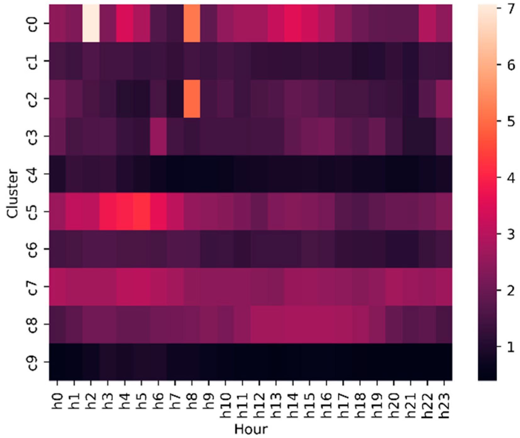
Moreover, employing the E2E learning model involves calculating the MAPE for every hour of the day across all clusters within the hierarchy. This is aimed at assessing the model’s performance across various time periods throughout the day. Figure 7 illustrates a heatmap showing the MAPE for all clusters across the 24 h of the day. The color gradient on the right indicates the MAPE, where lighter colors represent higher MAPE indicating lower accuracy. For each hour of the day, the MAPE for every cluster is below 5%, except for clusters 0, 2, and 5, which exhibit MAPE values of 7.06%, 4.98%, and 4.19% at 2 a.m., 8 a.m., and 5 a.m., respectively. Thus, the proposed methodology has an overall MAPE of less than 10% for every cluster in 24 h indicating that this model performs superior to other models.

4.5. Comparison between E2E Model and BU Approach

This E2E learning model is based on the principles of the TD approach. In contrast, the other widely used approach is the BU approach, which requires having individual local models for each group. This section compares the proposed E2E learning model with the conventionally used BU approach. The BU approach necessitates independent forecast models for each cluster, employing only features pertinent to each specific cluster. Therefore, features are chosen to reflect the unique characteristics of each individual cluster along with calendar variables. In the BU approach, utilizing aggregated-level features is deemed inappropriate as it deviates from the essence of the BU approach.

The individual models used for the BU approach are also based on neural networks consisting of cluster features and calendar variables. The cluster features used are the same as those of the E2E learning model. The results of individual forecast models were summed up to estimate the forecast at the aggregated level. The results are shown from both approaches and are presented in

Table 5. Comparison between E2E and BU approach.

Cluster	MAPE (%)
	E2E Model	BU
C0	3.4	15.22
C1	1.12	10.21
C2	5.4	14.7
C3	3.49	14.28
C4	2.6	11.19
C5	1.37	14.5
C6	2.07	13.97
C7	0.88	10.51
C8	1.71	14.78
C9	0.71	8.76

. The MAPE using local models is quite high compared to the proposed model with cross-learning features. The reasons are as follows.

According to the existing literature, the BU approach demonstrates superior performance compared to the TD approach when it comes to forecasting load at the sub-levels of a hierarchy. However, it comes at the cost of requiring substantial additional data to ensure accuracy. For residential a consumption forecast, BU uses physics-based models and behavior-related input features. The physics-based model uses principles of physics, such as appliance specification, energy consumption, operating hours, and usage patterns, along with the habits of residents, to explain the consumption [51]. However, in practical cases, it is not always possible to obtain such detailed data to be added as input features for improving the performance of the BU approach. Conversely, smart meters provide valuable insight into consumption and are recognized as valuable tools to enhance forecasting accuracy as shown in the proposed model. The proposed end-to-end (E2E) model leverages historical consumption data to extract features, employing cross-learning information from various hierarchy levels to enhance forecasting accuracy.

Figure 8 shows the comparison of the MAPE at the aggregated level for 24 h between the E2E model and BU approach. The proposed E2E model has a MAPE range of 0.08% to 1.85% in 24 h, while the BU approach has a range of 0.04% to 18.3%. The E2E model follows the actual values closely, while the BU approach deviates more. The E2E approach achieves high accuracy at the aggregated level because the TD approach is very precise at the aggregated level.

Thus, the proposed model exhibits resilience across various clusters, highlighting its adaptability in managing different patterns among clusters. Nevertheless, it is crucial to acknowledge that although the model’s structure and features remain uniform, retraining is essential to enhance performance within each cluster. This requirement stems from the inherent diversity among clusters, where distinct attributes and patterns prevail. Despite the imperative for retraining, our model consistently attains high accuracy rates across diverse clusters, affirming its efficacy and versatility. This serves as proof of concept that the proposed model, with its cross-learning capabilities, holds promise for applications in residential settings across different countries.

5. Discussion

This study develops and evaluates an E2E learning model for the residential hierarchical structure. The hierarchical load-forecast model is based on the principles of TD approach, which is less common than the BU approach for hierarchical models. However, BU-based models require the detailed features of each cluster involved in the hierarchy, making practical implementation difficult. This model utilizes features derived from historical load data, calendar variables, and specific features that explain the relationship between the aggregated level of hierarchy and the cluster requiring forecasts. This section discusses the performance of the model and a comparison against existing models, highlights the strengths and limitations, and suggests avenues for future research.

This model achieved promising results, with a mean absolute percentage error (MAPE) of less than 6% for all clusters in the hierarchy. This level of accuracy is not achieved by traditionally used statistical methods, such as SARIMA or SVR, for all of the involved clusters. Additionally, these methods require hyperparameter tuning for each cluster, whereas the proposed model performs well for all clusters without individual hyperparameter tuning. Incorporating the E2E model with cross-learning features allows this model to capture different patterns of different clusters, enabling a single model to provide accurate forecasts for all involved clusters.

Most existing hierarchical load-forecast models focus on the BU approach, where forecasts are made at lower hierarchy levels and then aggregated to higher levels. Although this approach leads to reasonable accuracy, it involves voluminous data that are difficult to handle in real-life scenarios. Moreover, this approach often suffers from bias and incoherence in forecasting. The proposed E2E learning model not only outperforms in accuracy but also uses input features derived solely from historical load data without needing any exogenous features. The results presented demonstrate the superior accuracy of the proposed E2E model, showing improvements in the mean MAPE compared to SARIMA, SVR, and the commonly used bottom-up hierarchical model by 91%, 85.8%, and 82.24%, respectively.

Each cluster in the hierarchy has a unique load profile, and one of the key strengths of the proposed model is its adaptability for different clusters without the need to change the model’s architecture and hyperparameters. However, the model has limitations. Firstly, the forecast accuracy may be affected by sudden extreme changes in data. Although the same model architecture and hyperparameters work well for all clusters, separate training is required for each cluster. Another challenge is the need for a large amount of historical data to train the model effectively, which can be difficult for smaller utilities with limited data access.

Future research in load forecasting could explore several avenues to further improve accuracy and efficiency, firstly, incorporating deep neural networks, like Long Short-Term Memory (LSTM), for sequence load forecasting. Additionally, testing the model on other datasets will assess the generalization ability of the model. As we look forward, we intend to expand the purview of this research to assess varying scenarios. Specifically, we aim to explore the integration of EVs and gauge its consequential impact on the model’s forecasting capability.

Despite these limitations, this study contributes to load forecasting by demonstrating the efficacy of an E2E learning model with cross-learning features in improving accuracy for hierarchical load structures, thereby reducing the computational burden. In conclusion, the study presents a robust load-forecast model that leverages machine learning to predict electricity demand with high accuracy. While challenges exist, this research highlights the potential of advanced forecasting techniques in shaping energy management and sustainability.

6. Conclusions and Future Work

The evolution of the power sector from regulated to deregulated has emphasized the need for adaptable solutions to accommodate these rapid transformations. Among the many challenges, accurately estimating demand stands out as a critical imperative, necessitating the development of robust load-forecast models. This study is dedicated to building an E2E learning model tailored to the residential hierarchical load structure. Constructing this hierarchical framework entails a thorough analysis of smart meter data from residential consumers, followed by the creation of seasonal representative load profiles for individual households. The foundation of the E2E learning model lies in its adherence to the fundamental principles of the top-down hierarchical approach. Leveraging features from various levels of hierarchy and integrating cross-learning information, this model is engineered to enhance forecast accuracy significantly. A distinctive feature of this model is its ability to forecast load at any node within the hierarchy, drawing upon input features from both the aggregated level and the specific node under consideration.

To ascertain the efficacy of the proposed E2E model, comparisons were conducted against the two-stage approach and other conventional methodologies. The findings underscore the superior performance of the E2E model, yielding forecasts with a MAPE of 2.27%, a notably lower margin compared to alternative methods. In showcasing the potential of the top-down concept, a comparative analysis with the bottom-up approach revealed a mean MAPE of 12.81% across all clusters using the BU approach. This evident contrast underscores the inherent advantages offered by the E2E model in terms of accuracy and efficiency. The versatility of the proposed single E2E learning model, capable of encompassing the entire hierarchy, holds paramount importance for stakeholders across the power sector. By providing accurate forecasts at every level of the hierarchy, this model empowers stakeholders with invaluable insights, facilitating informed decision-making and efficient resource allocation.