Optimized Decision-Making for Multi-Market Green Power Transactions of Electricity Retailers under Demand-Side Response: The Chinese Market Case Study

Abstract

With the energy structure transition and the development of the green power market, the role of electricity retailers in multi-market green power trading has become more and more important. Particularly in China, where aggressive green energy policies and rapid market transformations provide a distinct context for such studies, the challenges are pronounced. Under demand-side response, electricity retailers face the uncertainty of users’ electricity consumption and incentives, which complicates decision-making processes. The purpose of this paper is to explore the optimization decision-making problem of multi-market green power trading for electricity retailers under demand-side response, with a special focus on the Chinese market due to its leadership in implementing substantial green energy initiatives and its potential to set precedents for global practices. We first construct a two-party benefit optimization model, which comprehensively considers the profit objectives for electricity retailers and utility maximization for users. Then, the model is solved by the Lagrange multiplier method and distributed subgradient algorithm to obtain the optimal solution. Finally, the effectiveness of the incentive optimization strategy under the multi-market to promote green power consumption and improve the profit of electricity retailers is verified by arithmetic simulation. The results of this study show that the incentive optimization strategy under multi-market, particularly within the Chinese context, is expected to provide a reference for electricity retailers to develop more flexible and effective trading strategies in the green power market and to contribute to the process of promoting green power consumption globally.

1. Introduction

The global shift towards sustainable development has increasingly influenced energy policies, emphasizing the integration of environmental, economic, and social considerations to ensure long-term viability [1]. The concept of sustainable development in energy transactions necessitates a combined approach of technological advancements and economic principles for balanced growth. On 27 September 2023, China’s National Development and Reform Commission (NDRC) and six other departments released the ‘Measures for Electricity Demand Side Management (2023 Edition)’, which proposes to strengthen demand-side response (DSR) capabilities and increase the proportion of green electricity consumption [2]. This significant policy update, reflecting China’s commitment to sustainable energy practices, positions the Chinese electricity market as an ideal case study for this research. With the implementation of the new measures, participants in the electricity market are facing unprecedented opportunities and challenges, while the market demand and the behavioral patterns of electricity consumers have experienced significant shifts. Therefore, focusing on China provides a pertinent and timely examination of these dynamics in a context where green power initiatives are both mature and actively evolving, exemplifying a model of sustainable development in action.

As a key medium in the electricity market, electricity retailers can effectively guide electricity consumers to optimize their electricity consumption patterns by selling green electricity to them in conjunction with the implementation of well-designed incentives. This strategy not only enhances customer satisfaction and improves the market competitiveness of electricity retailers, but also promotes the widespread consumption of green electricity, which is of great practical significance for promoting the energy transition and realizing the goal of sustainable development.

Existing literature on green power trading and demand-side response covers a range of topics. Studies indicate that household green power trading could contribute significantly to carbon emission reductions [3]. Various approaches have been proposed to assign value to green electricity [4], determine willingness to pay [5], and to optimize tradable green certificate prices [6]. Other research explores the impact of green bonds, energy price volatility [7], and hydrogen production from green electricity [8]. New energy market models [9,10], optimization strategies [11], and blockchain-based mechanisms have also been proposed to enhance green power trading, particularly in China [12]. DSR plays a crucial role in power systems. Research suggests using price incentives and deep learning algorithms to improve load profiles and consumer response depths [13,14]. Techniques like recurrent neural networks and resilient distributed controllers mitigate risks like fake data injection attacks [15,16,17]. Price-based DSR, the participation of retailers with energy storage systems, and innovative schemes like coupon-based response have been explored as well [18,19,20]. Additionally, incorporating consumer psychology and blockchain technology offers promising avenues for advancing DSR programs, ensuring their effectiveness and sustainability [21,22]. Although the above literature has extensively explored the role of demand-side response and green power in the electricity market, most of the studies focus mainly on the proof of concept of DSR and the application of a single market, while less consideration has been given to how to effectively combine demand-side response strategies with multi-market trading, and, further, techniques for incentivizing demand-side response have not been adequately studied.

The Markov Decision Process (MDP) is crucial for advancing smart energy management and adeptly navigating the complexities and uncertainties of modern energy systems. MDP plays a significant role in facilitating strategic energy management across coordinated smart buildings and in incorporating advanced machine learning techniques to enhance cost-effectiveness and user satisfaction in smart facilities [23,24]. Additionally, the application of MDP extends to renewable energy integration, optimizing operations at photovoltaic-assisted electric vehicle charging stations and in-home energy systems [25,26]. These approaches adeptly manage real-time energy demands and pricing while adapting to user behaviors and dynamic market conditions. In the realm of smart grid and home energy management, MDP is instrumental in developing cost-effective pricing strategies and demand response programs, demonstrating remarkable flexibility in adapting to user preferences and fluctuating energy scenarios [27,28,29]. Together, these applications highlight the robustness of MDP in boosting the efficiency and sustainability of energy management across various domains.

In this study, the MDP is used to represent the uncertainty of user electricity consumption and incentives; the optimal decision model is then constructed to maximize the benefits of electricity sales and user utility. The model is solved by the Lagrange multiplier method and distributed sub-gradient algorithm, and finally, the simulation of the example shows that the real-time incentive optimization strategy can effectively improve the profit of the electricity retailers and promote the consumption of green electricity in a multi-market environment.

2. Methodology

2.1. Analysis of Response Uncertainty

The electricity consumption state of a customer is only related to the previous period and not to the previous electricity consumption state, which can be regarded as the ‘Markov property’ of the stochastic sequence.

The period time of a user’s electricity consumption is divided into 24 h: $h$ denotes the $h$th period of time, $I$ denotes the current user, and $i$ denotes each user. There are a total of $J$ users: $J$ denotes the set of users. $i\in J$ is denoted as $I^i(h)$ to represent the state space of the electricity consumption of user $i$ in period $h$. The state space of the electricity consumption of the user $i$ in period $h$ refers to the set of all possible electricity consumption behaviors of the user in that period. This includes the various electricity usage patterns of the consumer during that period, such as high load usage, low load usage, and outage status. This state space is useful for analyzing and predicting the electricity consumption behavior of the customer, which is essential for formulating targeted demand response measures and optimizing electricity sales strategies. $x^i(h)\in I^i(h)$ denotes the electricity consumption of user $i$ in period $h$. The electricity consumption of user $i$ in period $h$ refers to the total amount of electricity consumed by user $i$ in a specific period. This indicator is very important for the power system because it helps the power sales company or power management department to understand the demand for electricity in each period, better schedule the supply of electricity, and to regulate the operation of the power grid. Then:

$$\left\{I^i(h+1)=x^i(h+1)\left|\begin{array}{l}{I}^i(0)=x^i(0),I^i(0)=x^i(0),\\ \cdots I^i(h)=x^i(h),\end{array}\right.\right\}$$

(1)

The power consumption behavior of the user follows the Markov property; that is, the power consumption in each period only depends on the state of the previous period, and in any period, the power consumption $h$ of the user is limited, $x^i(h)\in \left[m^i(h),M^i(h)\right]$, $m^i(h)$ represents the total power consumption of the user due to the operation of the necessary equipment in the period of user $i$. $M^i(h)$ represents the electricity consumption required by user $i$ to turn on all electrical appliances during the $h$ period. The electric interval $\left[m^i(h),M^i(h)\right]$ is discretized and divided into $n$ states, denoted as $I^i(h)=\left\{x_1^i(h),x_2^i(h),\cdots x_n^i(h)\right\}$, where $x_1^i(h)=m^i(h)$, $x_n^i(h)=M^i(h)$. $f^i(h)={\left[f_1^i(h),f_2^i(h),\cdots f_n^i(h)\right]}^T\in {\left[0,1\right]}^n$ is the initial state; that is, the probability distribution of each power consumption state when it is sent to the user without incentive, and $f_k^i(h)\in \left[0,1\right],k=1,2,\cdots n$ represents the possibility of various possible power consumption behaviors of user $i$ in a specific period $h$. This involves the statistical analysis of user behavior patterns to estimate how often and regularly they use electricity over different periods.

The user will choose the electricity consumption state according to the incentive provided by the retailer, to determine the electricity consumption in the next period. This means that the user’s power consumption behavior can be adjusted through the incentive mechanism, to achieve the optimization of power consumption efficiency and the reasonable distribution of power resources. $P_{h,h+1}^i$ represents the probability $x^i(h+1)$ from the power consumption state $x^i(h)$ during period $h$ to the power consumption state $h+1$ during period $h$, which is expressed as $P_{h,h+1}^i=\mathrm{Pr}\{I^i(h+1)=x^i(h+1)\left|I^i(h)\right.=x^i(h)\}$.

The incentive that user $i$ receives from the electricity retailers in period $h$ is represented as ${\lambda }^i(h)$, and the incentive vector of $j$ users is $\lambda (h)={[{\lambda }^1(h),{\lambda }^2(h),\cdots ,{\lambda }^j(h)]}^T$. The state transition probability matrix describes the probability that the user will transfer from the current state of electricity consumption to the possible state of electricity consumption in the next period after receiving the incentive from the electricity retailers. This matrix can predict future electricity consumption behavior based on historical data and user behavior patterns, thus providing decision support for electricity retailers. Therefore, it can be expressed as

$$P_{h,h+1}^i({\lambda }^i(h))=\left[\begin{array}{ccc}{a}_{11}^i+b_{11}^i{\lambda }^i(h)& \cdots & a_{1n}^i+b_{1n}^i{\lambda }^i(h)\\ a_{21}^i+b_{21}^i{\lambda }^i(h)& \cdots & a_{2n}^i+b_{2n}^i{\lambda }^i(h)\\ ⋮& \ddots & ⋮\\ a_{n1}^i+b_{n1}^i{\lambda }^i(h)& \cdots & a_{nn}^i+b_{nn}^i{\lambda }^i(h)\end{array}\right]$$

(2)

Each element satisfies $0\le a_{de}^i+b_{de}^i{\lambda }^i(h)\le 1,d=1,2,\cdots n,f=1,2,\cdots n$, and each column satisfies ${\displaystyle {\displaystyle \sum _d^n}{a}_{de}^i+b_{de}^i{\lambda }^i(h)=1},f=1,2,\cdots n$.

The probability matrix of the user’s power consumption state takes into account a variety of influencing factors, and it represents the probability of the user moving from the current power consumption state to other possible states under different incentives. This matrix is usually modeled and analyzed based on the user’s electricity consumption history, incentive strategy effect, and external conditions.

$$\left[\begin{array}{c}{\omega }^1(h+1)\\ {\omega }^2(h+1)\\ ⋮\\ {\omega }^j(h+1)\end{array}\right]=\left[\begin{array}{cccc}{u}_{11}{P}_{h,h+1}^1\left({\lambda }^1(h)\right)& u_{12}E& \cdots & u_{1j}E\\ u_{21}E& u_{22}{P}_{h,h+1}^2\left({\lambda }^2(h)\right)& \cdots & u_{2j}E\\ ⋮& ⋮& \ddots & ⋮\\ u_{j1}E& u_{j2}E& \cdots & u_{jj}{P}_{h,h+1}^j\left({\lambda }^j(h)\right)\end{array}\right]\left[\begin{array}{c}{\omega }^1(h)\\ {\omega }^2(h)\\ ⋮\\ {\omega }^j(h)\end{array}\right]$$

(3)

2.2. Transaction Model Construction

2.2.1. Utility Function of Power Users

The relationship between the customer’s satisfaction and the degree of electricity consumption can be described by utility function, which is a common method in microeconomics. Utility function can reflect the satisfaction degree of users under different consumption levels and help to analyze and predict users’ preferences and responses to electricity consumption. The utility function $U(x,\pi )$ is commonly used, and the utility function must satisfy $\frac{\partial U(x,\pi )}{\partial \pi }>0$, $U(0,\pi )=0(\forall \pi >0)$.

$$U(x,\pi )=\left\{\begin{array}{l}\pi x-\frac{\alpha }{2}{x}^2,0\le x\le \frac{\pi }{\alpha }\\ \frac{{\pi }^2}{2\alpha },x>\frac{\pi }{\alpha }\end{array}\right.$$

(4)

2.2.2. Profit Function of Electricity Retailers under Demand-Side Response

In period $h$, the profit of an electricity retailer’s participation in demand-side response is determined by the combination of the cost of incentive compensation to customers, the cost of purchasing electricity, and the revenue from electricity sales. This profit function helps the retailer evaluate the economic benefits of implementing demand response, balance costs and benefits, and optimize its market strategy.

$$\begin{array}{l}{C}_{MO,h}=-C_{1,h}-C_{2,h}+C_{3,h}\\ C_{1,h}={\lambda }_h{\displaystyle {\displaystyle \sum }_{i=1}^N}{l}_{i,h}\\ C_{2,h}=P_h^{grid}{\gamma }_{1h}\Delta h+L(h){\gamma }_{2h}\\ C_{3,h}={\displaystyle {\displaystyle \sum }_{i=1}^N}{x}_{i,h}{\xi }_h\end{array}$$

(5)

In this formula, $C_{MO,h}$, $C_{1,h}$, $C_{2,h}$, and $C_{3,h}$ represent the profit of the seller participating in the demand response during period $h$, the incentive compensation cost issued to the user, the power purchase cost, and the electricity sales revenue generated by selling electricity to the user, respectively. ${\lambda }_h$ represents the incentive compensation price issued to users under the electricity retailer during period $h$. If the electricity retailers have no demand response plan, ${\lambda }_h$ is 0, and $l_{i,h}$ represents the response amount of users $i$ after receiving incentives from electricity retailers during period $h$. If the user does not participate in the response during this period, $l_{i,h}$ is 0, and $P_h^{grid}$ represents the power of green electricity purchased from green electricity generators during period $h$ in the spot market, ${\gamma }_{1h}$ represents the price of green electricity purchased from green electricity generators during period $h$ in the spot market, $L(h)$ represents the green electricity purchased by the seller from the spot market, ${\gamma }_{2h}$ represents the price of green electricity purchased by the seller during period $h$ in the spot market, $g_h$ represents the power purchased by the seller during the $h$ period, and $g_h\in \left[g_h^{\min },g_h^{\max }\right]$, where $g_h^{\max }={\displaystyle {\sum }_{i\in J}{M}_i^h}$ $g_h^{\min }={\displaystyle {\sum }_{i\in J}{m}_i^h}$; $\Delta h$, represents the unit optimization period. $X_{i,h}$ indicates the electricity consumption of user $i$ during period $h$, and ${\xi }_h$ represents the retail electricity price during period $h$.

The optimization model will take into account the cost minimization and user utility maximization of e-commerce vendors participating in demand response. The model is based on the MDP to optimize real-time excitation in multiple periods and to ensure the power supply and demand balance. Such a model can effectively guide e-commerce sellers to develop real-time dynamic incentive strategies to achieve dual optimal economic benefits and user satisfaction.

$$\begin{array}{l}\max E\left({\displaystyle {\displaystyle \sum }_{h=1}^T}\left[{\displaystyle {\displaystyle \sum }_{i=1}^N}{C}^i\left(x_h^i,{\pi }_h^i\right)-C_{MO,h}\left|x^i(0)=x_0^i\right.\right]\right)\\ s.t.(1)\sim (3)\end{array}$$

(6)

In this simulation, it is considered that green electricity needs to be purchased from the spot market when the hybrid electricity purchased by electricity retailers in the medium and long-term market faces an imbalance between supply and demand. $L(h)$ is used to represent the green electricity purchased by the electricity retailers in the spot market during period $h$. Therefore, constraints are added to the objective function:

$${\displaystyle \sum _{i=1}^J{\left(X_h^i-L_h^i\right)}^{+}}\le P_h^{grid}\Delta h$$

(7)

In this formula, ${\left[·\right]}^{+}$ represents the plus function, and the convention ${\left[x\right]}^{+}=\max \left\{x,0\right\}$. This constraint means that, to avoid the imbalance between supply and demand, the electricity selling company needs to ensure that the amount of electricity purchased from the grid is greater than the total amount of electricity sold to the end user when conducting electricity transactions. This is done to ensure the reliability of the power supply and to meet sudden power demand, while also allowing flexibility and a margin of safety for the company’s operations.

3. Model Optimization and Solution

The objective function (6) is converted into two parts for solving.

$$E\left[{\displaystyle \sum }_{i=1}^J{C}_i\left(x_h^i,{\pi }_h^i\right)-C_{MO,h}\right]={\displaystyle \sum }_{i=1}^J{C}_i\left(x_h^i,{\pi }_h^i\right)-C_{MO,h}$$

(8)

$$E\left[{\displaystyle \sum }_{h=k+1}^H\left[{\displaystyle \sum }_{i=1}^J{C}_i\left(x_h^i,{\pi }_t^i\right)-C_{MO,h}\right]\right]={\displaystyle \sum }_{h=k+1}^T\left[{\displaystyle \sum }_{i=1}^J{C}_i\left(x_h^i,{\pi }_h^i\right)-C_{MO,h}\right]$$

(9)

Because the actual electricity consumption of the user during each period usually does not reach the set maximum, the seller needs to consider this variability when purchasing electricity to ensure that it can meet the needs of the user without wasting resources. Therefore, it is necessary to determine the specific expression of $E\left[C_i\left(x_h^i,{\pi }_h^i\right)\right]$ in the case of $0<x_h^i<\frac{{\pi }_h^i}{{\alpha }_i}$, $i\in N$, $h=k+1,k+2,\cdots ,H$.

From Equation (7), this uncertainty can be handled by applying Chebyshev’s inequality when faced with constraints containing a random variable $L_h^i$. This approach helps to convert the constraints of the random variable into a deterministic form for more efficient processing and computation in the optimization model.

$$\mathrm{Pr}\left[{\displaystyle \sum }_{i=1}^N{\left(x_h^i-L_h^i\right)}^{+}-P_h^{grid}\mathsf{\Delta }\mathrm{h}\ge \eta \right]\le \epsilon$$

(10)

where: $\eta \ge 0$, Equation (10) denotes the difference between the amount of power required by the customer and the amount of power purchased by the seller from the generator in the current period, and is usually set to a pre-determined constant, which reflects the fluctuations in power demand and reserve capacity requirements that are taken into account by the electricity retailers in planning the purchase of power. $\epsilon$ denotes the probability that the power purchased by the electricity retailers will not be able to satisfy the demand of the customer, and this probability is usually set to a very small positive number to ensure that the system’s reliability and customer power demand are met.

An efficient way to solve the modeling problem is to utilize the Lagrangian function. This approach involves integrating constraints into the objective function to form a Lagrangian function, which, in turn, solves the original problem by finding the extreme points of this function. This process not only optimizes the efficiency of problem solving, but is especially effective when dealing with complex problems that contain multiple constraints:

$$\begin{array}{l}\begin{array}{l}\Gamma (X,P,\lambda ,p)={\displaystyle {\displaystyle \sum }_{h=k}^H}\left[{\displaystyle {\displaystyle \sum }_{i=1}^J}{C}_i\left(x_h^i,{\pi }_h^i\right)-C_{MO,h}\right]-{\displaystyle {\displaystyle \sum }_{i=1}^J}{p}_i\left[d^i-{\displaystyle {\displaystyle \sum }_{h\in H}}{x}_h^i\right]-{\lambda }_h\left[{\displaystyle {\displaystyle \sum }_{i=1}^J}{x}_h^i-P_h^{grid}\mathsf{\Delta }\mathrm{h}\right]\\ -{\displaystyle {\displaystyle \sum }_{h=k+1}^H}{\lambda }_{h}F\left(x_h^i,P_h^{grid}\mathsf{\Delta }\mathrm{h},e\right)\end{array}\hfill \end{array}$$

(11)

where ${\lambda }_h>0$ represents the incentive, $P_i(h\in H,i\in J)$ represents the Lagrange multiplier, $X=(X_h^i,i\in N,h\in H)$, $P=(P_h^{grid},h\in H)$, $\lambda =({\lambda }_h,h\in H)$, $P=(P_i,i\in J)$, and $P$ is the local multiplier, taking into account the specific constraints. Another expression can be used to describe the process wherein the optimization is implemented within a specific constraint framework. $\lambda$ is the global multiplier, taking into account the overall constraint framework for the analysis, representing the electricity consumption data in the model, which is also the goal of our study (that is, the multi-temporal coupling of the incentives), and $e$ denotes an extremely small positive number, similar to the value of $\epsilon$ above.

$$S\left(\lambda ,p\right)=\underset{x_h^j,p_h^{\mathrm{grid}}\in \left[m_h,M_h\right]}{\max }\Gamma \left(X,P,\lambda ,p\right)=\sum _{h=1}^J{G}_i\left(\lambda ,p_i\right)+D\left(\lambda \right)$$

(12)

where $p_i$, $i\in N$, and

$$\begin{array}{l}{G}_i(\lambda ,p_i)=\underset{x_h^i}{\max }{\displaystyle \sum _{h=K}^H{C}_i}(x_h^i,{\pi }_h^i)-p_i[d^i-{\displaystyle \sum _{h\in H}{x}_h^i]}-{\lambda }_h{x}_h^i-{\displaystyle \sum _{h=K+1}^H{\lambda }_h[{(x_h^i)}^2+2\sqrt{{{\displaystyle \stackrel{\Lambda }{\mu }}}_2^2}}{x}_h^i\\ +x_h^i+\sqrt{{{\displaystyle \stackrel{\Lambda }{\mu }}}_1^2}+{\stackrel{\Lambda }{\sigma }}_1^2+{{\displaystyle \stackrel{\Lambda }{\mu }}}_2^2+\frac{1}{N\sqrt{2\epsilon }}\stackrel{\Lambda }{{\sigma }_1}\sqrt{N+2N{\left(\stackrel{\Lambda }{{\sigma }_1}\right)}^2}]\end{array}$$

(13)

$$D(\lambda )=\underset{P_h^{grid}\in \left[m_h,M_h\right]}{\max }{\lambda }_h{P}_h^{grid}\mathsf{\Delta }\mathrm{h}+{\displaystyle \sum }_{h=k+1}^{H}2e{\lambda }_h\left(P_h^{grid}\mathsf{\Delta }\mathrm{h}+\eta \right)-{\displaystyle \sum }_{h=k}^H{C}_{MO,h}$$

(14)

translates into the dyadic problem of solving the objective function Equation (6):

$$\underset{\lambda >0}{\min }S(\lambda ,p)$$

(15)

From the derivation process, it is evident that the objective function meets the conditions of Lagrange’s strong dyadic theorem, so the original objective function can be solved by solving the dyadic problem instead of solving the original objective function directly, which can simplify the solution process under certain conditions.

The distributed gradient algorithm is used to solve the dyadic problem of the objective function, which allows the user side and the electricity retailers to optimize independently. Once the optimal solutions $X_h^{i*}$ and $p^{*}$ are derived from the algorithm, the electricity retailers update the real-time incentive mechanism across multiple periods to optimize the overall power trading strategy.

When $h=k$

$${\lambda }_k^{v+1}={\left[{\lambda }_k^v-{\theta }_k\frac{\partial D\left({\lambda }^v,p^v\right)}{\partial {\lambda }_k^v}\right]}^{+}={\left[{\lambda }_k^v+{\theta }_k\left({\displaystyle \sum }_{i=1}^N{x}_k^{i\ast }\left({\lambda }^0,p_i^v\right)-P_k^{\ast }\left({\lambda }_k^v\right)\right)\right]}^{+}$$

When $h=k+1,k+2,\cdots ,H$

$$\begin{array}{l}{\lambda }_h^{v+1}={\left[{\lambda }_h^v-{\theta }_h\frac{\partial D\left({\lambda }^v,p^v\right)}{\partial {\lambda }_k^v}\right]}^{+}=\{{\lambda }_h^v+{\theta }_t[{\displaystyle \sum _{i=1}^J}{(x_h^{i\ast }({\lambda }^v,p_i^v)}^2+2\sqrt{{\widehat{\mu }}_2^2}{\displaystyle \sum _{i=1}^J}{x}_h^{i\ast }({\lambda }^v,p_i^v)+\\ {\displaystyle \sum _{i=1}^J}{x}_h^{i^{\ast }}({\lambda }^{\nu },p_i^{\nu })-2e(p_h^{\ast }({\lambda }_h^{\nu })+\eta )+N(\sqrt{{\widehat{\mu }}_1^2}+{\widehat{\sigma }}_1^1+{\widehat{\mu }}_2^2)+\frac{1}{\sqrt{2\epsilon }}{\widehat{\sigma }}_1\sqrt{N+2N{\widehat{\sigma }}_1^2}]{\}}^{+}\end{array}$$

The computation of the subgradient algorithm to update ${\beta }_i$ is publicized as follows:

$$p_i^{v+1}=p_i^v-{\beta }_i\frac{\partial D\left({\lambda }^v,p^v\right)}{\partial p_i^v}=p_i^v+{\beta }_i(d^i-\sum _{h\in H_i}{x}_h^i({\lambda }^v,p_i^v)),i\in J,$$

where $v$ is the number of iterations, and ${\theta }_h$ and ${\beta }_i$ are the iteration steps. The user side and electricity retailers interact with each other through information and updates $X_h^{i\ast }$, $p$, $\lambda$, and $p^{*}$ several times until the optimal solution is obtained.

From the above discussion, two parts, Algorithm 1 and Algorithm 2, which correspond to the user and the selling e-commerce company, respectively, are obtained as follows:

Algorithm 1 User $i$, $i\in N$, part of the computation

Step 1: Set the elasticity coefficient ${\pi }_h^i$ in the user function and the step size ${\beta }_i$ in the Lagrange multiplier iterative method, set the initial user state transfer probability, the Lagrange multiplier $p_i^v$, and the electricity consumption $x_h^i$, $h\in H$, and specify the termination error as $0<{\epsilon }_1<1$, $0<{\epsilon }_2<1$, and the number of iterations $v=0$;   Step 2: Obtain the incentive ${\lambda }^v$ from the electricity retailers;   Step 3: Solve the objective function using ${\lambda }^v$ and $p_i^v$ to obtain the electricity consumption $x_h^{i*}$, $h\in H$;   Step 4: Update the Lagrange multiplier $p_i^v$, denoted as $p_i^{v+1}$;   Step 5: The electricity retailers receive the new electricity consumption $x_h^{i*}$, $h\in H$;   Step 6: If $\left|{\lambda }^{v+1}-{\lambda }^v\right|<{\epsilon }_1$ and $\left|p_i^{v+1}-p_i^v\right|<{\epsilon }_2$ are satisfied, then the algorithm is complete and the optimal solution $x_h^{i*}$ is obtained; if not, update the number of iterations $v=v+1$ and return to Step 2.

Algorithm 2 The part calculated by the electricity seller

Step 1: Set the step size in the Lagrange multiplier iterative method ${\theta }_t$, assuming that the original incentive ${\lambda }^v$ is transmitted to each power user, and stipulate that the termination error is set to $0<{\epsilon }_1<1$, $0<{\epsilon }_2<1$, and the number of iterations $v=0$;   Step 2: Obtain the new electricity consumption under the incentive mechanism $x_h^{i*}$, $h\in H$;   Step 3: The incentive ${\lambda }^v$ is used to solve the objective function, and the solution can be obtained as the power sales $P^{\tau +1}\Delta h$;   Step 4: Recalculate the new incentive named ${\lambda }^{v+1}$;   Step 5: The updated incentive PP is transmitted to all power users;   Step 6: If both $\left|{\lambda }^{v+1}-{\lambda }^v\right|<{\epsilon }_1$, $\left|p_i^{v+1}-p_i^v\right|<{\epsilon }_2$ conditions are satisfied, then the algorithm is complete and the optimal solution is calculated ${\lambda }^{*}={\lambda }^{v+1}$, $P^{*}=P^{v+1}$; if not, update the iteration number $v=v+1$ and go back to Step 2 again.

4. Calculation Example Analysis

4.1. Basic Parameter Settings

In the setup of this study, the scenario under consideration involves one electricity retailer and 400 users. Here, the day is divided into 24 periods for power optimization on an hourly basis. The set limit of power purchase is based on the total amount of operation of the user’s equipment. Meanwhile, the elasticity coefficient of the user utility function varies between 10 and 11. In the pricing model, the purchased power price of the electricity retailer is set to a fixed RMB 0.49 per kWh, while its sales price to users is set to 70% of the cost price. Such a setup is intended to simulate a realistic electricity market trading environment.

${\mu }_1$ and ${\mu }_2$, which are set to 0 and 2, respectively, control some aspect of the utility function. ${\sigma }_1$ and ${\sigma }_2$, both set to 1, also affect the utility function. ${\alpha }_i$ is set to 0.25 and affects the power consumption of the user. $e$ is taken to be 0.1 and may involve energy losses or other factors. To investigate different incentive strategies, three different step parameters ${\theta }^h$ are set: 0.05, 0.001, and 0.0005 (

Table 1. Basic parameter settings.

Parameters	Numeric	Parameters	Numeric
${\mu }_1$	0	${\sigma }_2$	1
${\mu }_2$	2	${\alpha }_i$	0.25
${\sigma }_1$	1	$e$	0.1

).

4.2. Analysis of Incentive Convergence

When the step size ${\theta }^h=0.05$, the fast convergence from the larger iteration step size can be seen in Figure 1. In the initial stage, the excitation value rises rapidly, but as the number of iterations increases, it starts to stabilize, showing good convergence. An iterative process with a moderate step size can be seen when ${\theta }^h=0.001$. It converges slower than the green line but faster than ${\theta }^h=0.0005$. It presents a relatively smooth and stable convergence process. ${\theta }^h=0.0005$ represents an iterative process with a very small iterative step size, and it shows a very slow convergence process. It requires more iterations to reach a stable excitation value. The blue dashed line represents the optimal excitation value, which is the target value that the other lines try to reach during the iteration process. It is a fixed value that represents the optimal level of excitation that can be achieved within the given parameters and conditions.

As illustrated in Figure 1, larger iteration step sizes can reach convergence faster, but may result in the oscillation of excitation values rather than stabilization. Conversely, smaller iterative step sizes lead to slower convergence but can lead to smoother and more stable target values. The step size ${\theta }^h$ plays a key role in excitation convergence. By choosing an appropriate step size, it is possible to ensure that the system finds the optimal solution. A moderately sized step size of 0.001 performs most effectively.

4.3. Profit Analysis of E-Commerce Sales

4.3.1. Profit Analysis of Electricity Retailer under Different Incentives

Figure 2 shows the profit of electricity retailers with different incentives. When the demand-side response is not considered, the profit of the electricity retailer remains constant and does not change with the incentive price. This is because disregarding demand-side response usually implies that the revenues and costs of the electricity retailer are relatively fixed and do not fluctuate significantly in response to changes in market prices. The incentive price mainly affects the consumer or market participant’s behavior towards the use of electricity, especially the consumption and use of green power. If the business model and revenue structure of the electricity seller are not directly related to these changes, then changes in incentive prices will not have a significant impact on its profits. When demand-side response is considered, the profit of the electricity seller is in the low incentive price range [0, 6.23]. As the incentive price increases, the profit increases during the initial phase of customer demand-side response because the customer receive incentives issued by the electricity retailer and the electricity retailer sells more electricity, which increases the profit. As the incentive price increases to RMB 6.23/KWH, the profit of the electricity retailer reaches a peak of RMB 180,886, which indicates the point of the optimal combination of the incentive price and the effect of the demand response strategy, where the electricity retailer can obtain the maximum profit. After the profit peaks, the incentive paid by the electricity retailer to the customer exceeds the cost savings through demand response, and the electricity retailer’s profit begins to decline and eventually falls to a negative value. Overall, considering demand-side response increases the profitability of the retailer within a certain range of incentives, which is beneficial to the retailer’s operations.

4.3.2. Profit Analysis of Electricity Sellers in Different Markets under DSR

It can be seen in Figure 3 that, in the spot market considering the demand-side response, the profit of electricity retailers shows large fluctuations, which indicates that price fluctuations and changes in demand in the short term have a significant impact on profit. When responding to demand-side response in the medium- and long-term market, the profit of electricity retailers is more stable, reflecting the stability of profit due to medium- and long-term contracts and stable consumption rates. In the case of combining the spot and medium- and long-term markets, the profit fluctuations of electricity retailers fall in between, with both profit levels and volatility optimized. This suggests that the response speed of the market directly affects profits: the fast response of the spot market can bring timely profit adjustments for electricity retailers, while the stable response of the medium- and long-term market ensures the continuity of profits. In summary, through demand-side response, the seller can adjust its strategy faster in the spot market, while the medium- and long-term market provides a stable guarantee of profit, and the combination of the two provides the electricity retailer with an optimized solution that balances risk and return.

4.4. Analysis of Green Power Consumption Rate

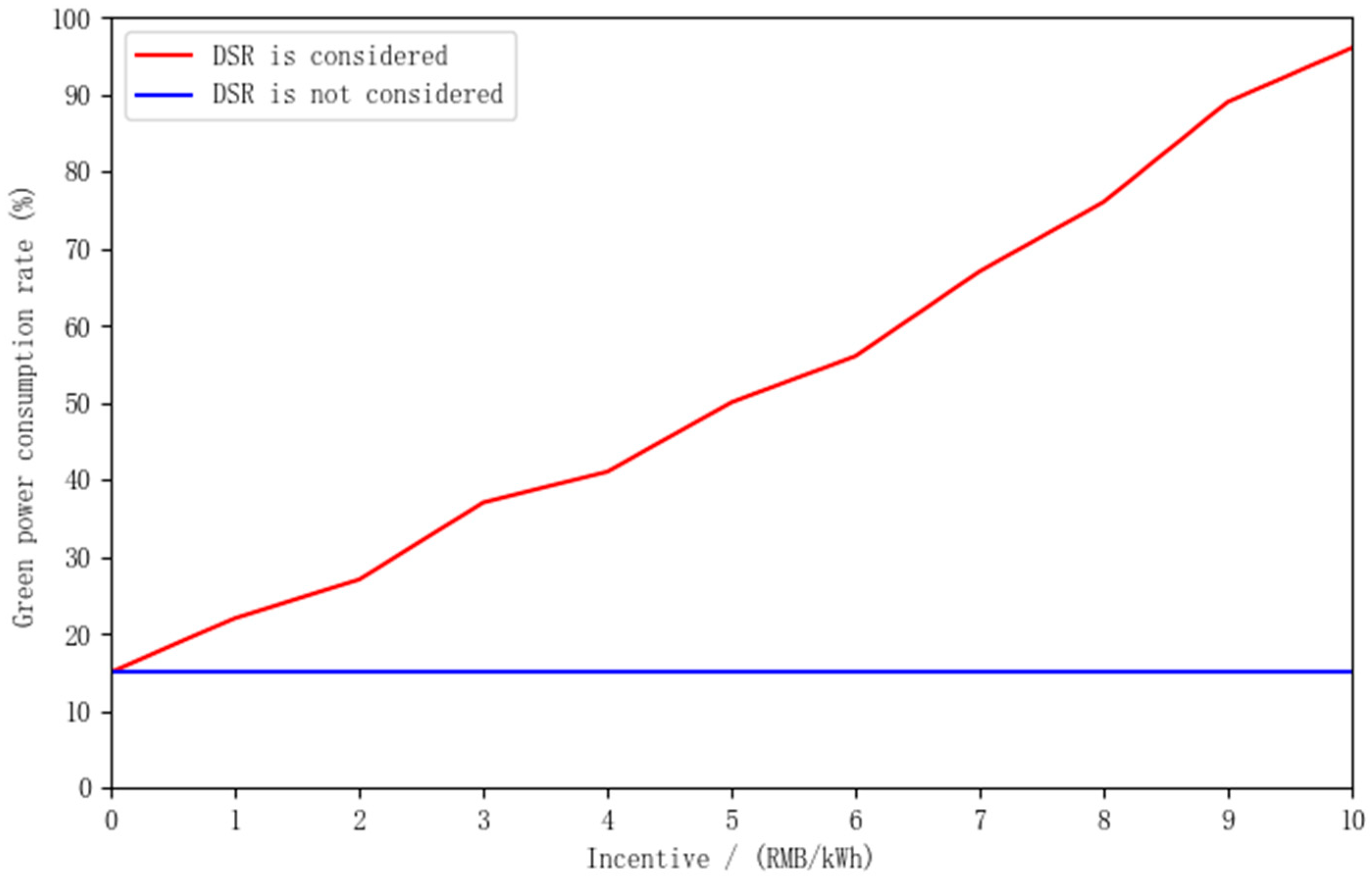
4.4.1. Analysis of Green Power Consumption Rate under Different Incentive Levels

Figure 4 shows the green power consumption rate under different incentive levels. Due to the constraints of the electricity retailer’s renewable energy quota system, the green power consumption rate stays constant when the demand-side response is not taken into account, and regardless of how the incentive price changes, the electricity retailer’s green power sales strategy remains fixed, and the electricity retailer has already reached the minimum green power consumption ratio stipulated in the policy. Since quota systems often specify a mandatory minimum consumption ratio, the electricity retailer may just be meeting this basic requirement without further increasing the consumption of green power. When considering the demand-side response, the green power consumption rate increases with the incentive price, and as the incentive price mechanism encourages more green power consumption, it causes the electricity retailer to exceed the minimum percentage of green power consumption specified by the quota system. Combined with this figure, we can analyze that the incentive strategy is an effective tool for promoting green power consumption beyond the minimum consumption ratio under the framework of the renewable energy quota system. Demand-side response measures can stimulate market demand and encourage consumers to buy more green power, thus helping electricity retailers to increase their green power consumption rate and achieve more aggressive environmental goals.

4.4.2. Analysis of Green Power Consumption Rate under Different Incentive Modes

The analysis in Figure 5 illustrates that combining incentives and demand-side response has a significant effect on improving the green power consumption rate. Real-time incentives combined with demand-side response is the most efficient because it can prompt electricity retailers and consumers to quickly adapt to the immediate changes in the market, while in the absence of a demand-side response mechanism, the enhancement of the green power consumption rate is limited even if real-time incentives are implemented. Therefore, a demand-side response strategy is indispensable for the optimization of green power trading, and it is particularly important in a multi-market environment to help electricity retailers optimize energy use and cost-effectiveness on different time scales.

4.4.3. Analysis of Green Power Consumption Rate in Different Markets under Demand-Side Response

Figure 6 illustrates that in the spot market, the green power consumption rate exhibits a significantly higher trend when considering the demand-side response. This is because of the high price volatility in the spot market, and demand-side response can adapt to the changes in price and green power supply by instantly adjusting consumption, especially during periods of low electricity price and high green power supply, which prompts an increase in electricity consumption and thus improves the green power consumption rate. For the medium-to-long-term market, the green power consumption rate is relatively stable, as this market is associated with long-term contracts and fixed prices. The demand-side response can help electricity retailers optimize green power purchasing and consumption strategies at the planning stage, keeping consumption rates stable to meet long-term contract requirements and renewable energy targets. Green power consumption rates are at their highest when a combination of spot and medium- and long-term markets are considered, demonstrating the advantages of cross-market adjustments. The demand-side response in this combined model can use the combination of price signals from the spot market and the stability of the medium- and long-term market to optimize the green power consumption rate. Therefore, the implementation of the demand-side response strategy can significantly improve the green power consumption rate in the spot market and maintain the stability of the consumption rate in the medium- and long-term market, while the combination of the two can further optimize the efficiency of the consumption, demonstrating that the cross-market demand-side response has significant advantages in improving the green power consumption rate.

5. Theoretical and Policy Implications

This study advances the theoretical framework of energy market optimization through the application of MDP and sophisticated algorithms like the Lagrange multiplier method and distributed subgradient algorithm, showcasing their efficacy in modeling the complexities of multi-market green power transactions and demand-side responses. The findings highlight the robustness of MDP in addressing the uncertainties inherent in energy systems, providing a solid foundation for future research. From a policy perspective, the results support the enhancement of DSR capabilities and advocate for regulatory frameworks that encourage the adoption of innovative energy management technologies. By demonstrating the effectiveness of incentive-driven DSR in the Chinese energy market, this research suggests that similar policies could be beneficial if adapted to other regional contexts, thereby promoting the global transition towards sustainable energy practices. Policymakers are encouraged to implement flexible incentive structures and foster public-private partnerships to accelerate the adoption of smart energy solutions, enhancing both market efficiency and sustainability.

6. Conclusions

This study focuses on the impact of demand-side response in the optimization decision of green power trading for electricity sellers in a multi-market environment. Through modeling analyses and empirical studies, the findings of this paper show that demand-side response strategies significantly enhance the green power consumption rate, with the strategy of real-time incentives combined with demand-side response being the most effective. This finding provides strategic guidance for electricity retailers on how to optimize green power trading under uncertain market conditions, emphasizing the importance of flexibility and timely responses to market dynamics. The paper similarly optimizes green power trading decisions for electricity retailers in a multi-market environment. Used in conjunction with spot and medium- and long-term markets, the demand-side response enables electricity retailer to maximize their profits while increasing green power consumption, which in turn, supports the widespread use of renewable energy and contributes to the economic and environmental sustainability of electricity markets.

However, this study also has certain shortcomings. First, the market environment of the study is set in a more idealized way, which does not fully reflect the irregularities and complexities of the real market. Second, the model in this paper has not yet taken into account the possible impacts of policy changes, market rule adjustments, and new technological developments on green power trading and demand-side response mechanisms. In addition, future research needs to further analyze the dynamics of different market participants’ behaviors and consider how to implement and manage incentive-based demand response mechanisms in reality.

In summary, although this study provides valuable theoretical insights and practical suggestions, further in-depth research and refinement are needed in practical applications to support more accurate and effective decision making by electricity retailers in the changing market environment.

References

1. Manioudis, M.; Meramveliotakis, G. Broad strokes towards a grand theory in the analysis of sustainable development: A return to the classical political economy. New Political Econ. 2022, 27, 866–878. [Google Scholar] [CrossRef]
2. National Development and Reform Commission. Notification on Issuing “Electricity Demand Side Management Methods (2023 Edition)”: Fa Gai Yun Hang Gui [2023] No. 1283 [EB/OL]. Available online: https://www.gov.cn/zhengce/zhengceku/202310/content_6907311.htm (accessed on 29 March 2024).
3. Lin, B.; Qiao, Q. Exploring the participation willingness and potential carbon emission reduction of Chinese residential green electricity market. Energy Policy 2023, 174, 113452. [Google Scholar] [CrossRef]
4. Gao, H.; Hu, M.; He, S.; Liu, J. Green electricity trading driven low-carbon sharing for interconnected microgrids. J. Clean. Prod. 2023, 414, 137618. [Google Scholar] [CrossRef]
5. Wimmers, A.; Madlener, R. The European market for guarantees of origin for green electricity: A scenario-based evaluation of trading under uncertainty. Energies 2023, 17, 104. [Google Scholar] [CrossRef]
6. Xu, S.; Xu, Q. Optimal pricing decision of tradable green certificate for renewable energy power based on carbon-electricity coupling. J. Clean. Prod. 2023, 410, 137111. [Google Scholar] [CrossRef]
7. Taghizadeh-Hesary, F.; Phoumin, H.; Rasoulinezhad, E. Assessment of role of green bond in renewable energy resource development in Japan. Resour. Policy 2023, 80, 103272. [Google Scholar] [CrossRef]
8. Notteboom, T.; Haralambides, H. Seaports as Green Hydrogen Hubs: Advances, Opportunities and Challenges in Europe. Marit. Econ. Logist. 2023, 25, 1–27. [Google Scholar] [CrossRef]
9. Johnathon, C.; Agalgaonkar, A.P.; Planiden, C.; Kennedy, J. A proposed hedge-based energy market model to manage renewable intermittency. Renew. Energy 2023, 207, 376–384. [Google Scholar] [CrossRef]
10. Sousa, J.; Lagarto, J.; Camus, C.; Viveiros, C.; Barata, F.; Silva, P.; Alegria, R.; Paraíba, O. Renewable energy communities optimal design supported by an optimization model for investment in PV/wind capacity and renewable electricity sharing. Energy 2023, 283, 128464. [Google Scholar] [CrossRef]
11. Wang, T.; Hua, H.; Shi, T.; Wang, R.; Sun, Y.; Naidoo, P. A bi-level dispatch optimization of multi-microgrid considering green electricity consumption willingness under renewable portfolio standard policy. Appl. Energy 2024, 356, 122428. [Google Scholar] [CrossRef]
12. Zhao, W.; Zhang, S.; Xue, L.; Chang, T.; Wang, L. Research on Model of Micro-grid Green Power Transaction Based on Blockchain Technology and Double Auction Mechanism. J. Electr. Eng. Technol. 2024, 19, 133–145. [Google Scholar] [CrossRef]
13. Wang, L.; Hou, C.; Ye, B.; Wang, X.; Yin, C.; Cong, H. Optimal operation analysis of integrated community energy system considering the uncertainty of demand response. IEEE Trans. Power Syst. 2021, 36, 3681–3691. [Google Scholar] [CrossRef]
14. Liu, D.; Qin, Z.; Hua, H.; Ding, Y.; Cao, J. Incremental incentive mechanism design for diversified consumers in demand response. Appl. Energy 2023, 329, 120240. [Google Scholar] [CrossRef]
15. Wen, L.; Zhou, K.; Li, J.; Wang, S. Modified deep learning and reinforcement learning for an incentive-based demand response model. Energy 2020, 205, 118019. [Google Scholar] [CrossRef]
16. Kong, X.; Kong, D.; Yao, J.; Bai, L.; Xiao, J. Online pricing of demand response based on long short-term memory and reinforcement learning. Appl. Energy 2020, 271, 114945. [Google Scholar] [CrossRef]
17. Yang, S.; Lao, K.W.; Chen, Y.; Hui, H. Resilient distributed control against false data injection attacks for demand response. IEEE Trans. Power Syst. 2024, 39, 2837–2853. [Google Scholar] [CrossRef]
18. Fleschutz, M.; Bohlayer, M.; Braun, M.; Henze, G.; Murphy, M.D. The effect of price-based demand response on carbon emissions in European electricity markets: The importance of adequate carbon prices. Appl. Energy 2021, 295, 117040. [Google Scholar] [CrossRef]
19. Yang, S.; Tan, Z.; Liu, Z.; Lin, H.; Ju, L.; Zhou, F.; Li, J. A multi-objective stochastic optimization model for electricity retailers with energy storage system considering uncertainty and demand response. J. Clean. Prod. 2020, 277, 124017. [Google Scholar] [CrossRef]
20. Gul, S.S.; Suchitra, D. A multistage coupon incentive-based demand response in energy market. Ain Shams Eng. J. 2024, 15, 102468. [Google Scholar] [CrossRef]
21. Shen, Y.; Li, Y.; Zhang, Q.; Li, F.; Wang, Z. Consumer psychology based optimal portfolio design for demand response aggregators. J. Mod. Power Syst. Clean Energy 2021, 9, 431–439. [Google Scholar] [CrossRef]
22. Mao, X.; Xue, M.; Zhang, T.; Tan, W.; Zhang, Z.; Pan, Y.; Wu, H.; Lin, Z. Centralized bidding mechanism of demand response based on blockchain. Energy Rep. 2022, 8, 111–117. [Google Scholar] [CrossRef]
23. Tsaousoglou, G.; Efthymiopoulos, N.; Makris, P.; Varvarigos, E. Multistage Energy Management of Coordinated Smart Buildings: A Multiagent Markov Decision Process Approach. IEEE Trans. Smart Grid 2022, 13, 2788–2797. [Google Scholar] [CrossRef]
24. Lu, R.; Bai, R.; Luo, Z.; Jiang, J.; Sun, M.; Zhang, H.T. Deep Reinforcement Learning-Based Demand Response for Smart Facilities Energy Management. IEEE Trans. Ind. Electron. 2022, 69, 8554–8565. [Google Scholar] [CrossRef]
25. Wu, Y.; Zhang, J.; Ravey, A.; Chrenko, D.; Miraoui, A. Real-time Energy Management of Photovoltaic-Assisted Electric Vehicle Charging Station by Markov Decision Process. J. Power Source 2020, 476, 228504. [Google Scholar] [CrossRef]
26. Xu, X.; Jia, Y.; Xu, Y.; Xu, Z.; Chai, S.; Lai, C.S. A Multi-Agent Reinforcement Learning-Based Data-Driven Method for Home Energy Management. IEEE Trans. Smart Grid 2020, 11, 3201–3211. [Google Scholar] [CrossRef]
27. Lu, T.; Chen, X.; McElroy, M.B.; Nielsen, C.P.; Wu, Q.; Ai, Q. A Reinforcement Learning-Based Decision System for Electricity Pricing Plan Selection by Smart Grid End Users. IEEE Trans. Smart Grid 2021, 12, 2176–2187. [Google Scholar] [CrossRef]
28. Yu, L.; Xie, W.; Xie, D.; Zou, Y.; Zhang, D.; Sun, Z.; Zhang, L.; Zhang, Y.; Jiang, T. Deep Reinforcement Learning for Smart Home Energy Management. IEEE Internet Things J. 2020, 7, 2751–2762. [Google Scholar] [CrossRef]
29. Chen, S.J.; Chiu, W.Y.; Liu, W.J. User Preference-Based Demand Response for Smart Home Energy Management Using Multiobjective Reinforcement Learning. IEEE Access 2021, 9, 161627–161637. [Google Scholar] [CrossRef]
Figure 1. Comparison of excitation convergence effect with different step sizes.
Energies 17 02543 g001
Figure 2. Profit of selling e-commerce under different incentives.
Energies 17 02543 g002
Figure 3. Profit analysis of different markets for selling electricity under demand-side response.
Energies 17 02543 g003
Figure 4. Green power consumption rate under different incentive levels.
Energies 17 02543 g004
Figure 5. Comparison of green power consumption rates under different incentive models.
Energies 17 02543 g005
Figure 6. Green power consumption rate in different markets under demand-side response.
Energies 17 02543 g006