Nonlinear Impact of Topological Configuration of Coupled Inverter-Based Resources on Interaction Harmonics Levels of Power Flow

Abstract

The increasing level of harmonics in the power grid, driven by a substantial presence of coupled inverter-based energy resources (IBRs), poses a new challenge to power grid transient stability. This paper presents the findings from experiments and analytical studies on the impact of the topological configuration of coupled IBRs on the level of power flow harmonics in a distribution grid: (i) our findings report that the impact of grid topology on harmonics is nonlinear, which is in contrast to the common perception that the power grid operates as a large linear low-pass filter for harmonics; (ii) importantly, this study highlights that the influence of the topological configuration of inverters on the reduction of system-level harmonics is more substantial than the effect of line impedance, emphasizing the significance of grid topological configuration; (iii) furthermore, the observed reduction in harmonics is attributed to a harmonic cancellation effect achieved through self-compensation by all the coupled inverters without affecting the active power flow in the power grid. These findings propose a new approach to limit the penetration of complex IBR harmonics in the power grid from a system-wide perspective. This approach significantly differs from the component-level or localized solutions used today, such as inverter control, power filtering, and transformer tap changes.

1. Introduction

1.1. Current State-of-the-Art

High penetration of inverter-based resources will increase the amount of harmonics in power flows in the power grid, which can cause various complex stability issues. These are important ways that harmonics from high penetration of inverter-based resources can negatively impact power system angle stability and voltage stability, as highlighted in references [1,2,3,4,5]. The majority of advanced techniques proposed, developed, and implemented to reduce harmonics in response to this challenge are component or local-level solutions achieved by controlling the IGBT switching strategy and topology of inverters, blocking high-frequency components with power filters, and shifting the phase of IBRs via transformer tap changing.

As an example of inverter control, in [6], a control strategy was put forth for designing sequence-asymmetric systems with the aim of locally correcting harmonic voltage issues. In [7], the authors present a technical idea that integrates a nearest-level controller with selective harmonic elimination control to improve the quality of the inverter’s output terminal voltage while minimizing harmonic distortion; a new hybrid frame controller is introduced, where the synchronous frame is utilized for the adaptive harmonic compensatory in the grid-connected inverter [8]; in [9], the article proposes a novel filter, which effectively attenuates harmonics with small inductance for grid-connected inverters. Generally, control-based methods focus on active power sources by regulating the switching patterns of inverters. These methods are designed to provide localized control to reduce harmonic levels on the source side. The filter-based approach is to design passive filters at the inverter output, aiming to block high-frequency components from entering the power lines and the circuit of the power grid. Typically, passive elements such as LCL or LC filters are employed. These methods normally are not very economical as they will increase the cost for integration of IBRs and have the risk of inducing undesired or detrimental complex transients such as harmonic resonance and inrush currents, as reported in [10,11].

Appropriate shifting of the phases of inverters is an emerging technical approach that has shown its effectiveness. By strategically adjusting the relative phase angles among coupled IBRs via the tap setting of the coupling transformer, this technique enables interconnected inverters to mitigate each other’s harmonics, resulting in a substantial reduction in power flow harmonics. The effectiveness of this technique was reported in [12]. Many works following this phase-shifting idea have been reported. For example, in [13,14], a different low-frequency hybrid modulation technique is proposed to incorporate phase shift in pulse width modulation (PS-PWM) and asymmetric selective harmonic current mitigation PWM (ASHCM-PWM) to reduce harmonics.

The concept of phase-shifting is specifically discussed in [15], which explains the relation between harmonics reduction and phase displacements from a perspective of coupled IBRs, as well as the nonlinear effect of cancellation interactions of IBRs.

1.2. Contribution of the Paper

Most existing methods to address the challenge of limiting the proliferation of harmonics to power grids to meet predefined design and compatibility standards for integrating IBRs to power grids are typically resource-side technologies using either component-level or local solutions. This paper presents the findings of experimental results as well as analytical studies, suggesting a possible approach from a system perspective. This approach is novel in that it offers a solution to limit the penetration of the harmonics from the system perspective, different from the component level or local solutions used today. Adjusting the topological configuration does not need to increase the cost of the power grid and will not change the active power flows. Thus, it can be seen as a low-cost and $free$ technical option for harmonic reduction as it engineers self-compensation interactions of coupled inverters in the same sense of harmonics cancellation through phase-shifting as described in [15].

1.3. Paper Organization

The remainder of the paper is organized as follows: Section 2 provides an analytical explanation of how the topological configuration affects harmonics. Section 3 introduces the experimental hardware employed in this paper, along with the primary experimental findings and discussions regarding the influence of electrical distance on total harmonic distortion. Section 4 is dedicated to the presentation of further experimental studies. Finally, in Section 5, the concluding remarks of this paper are presented.

2. Analytical Explanation of the Relationship between Harmonics and Topological Configuration in Power Systems

In this section, we start by explaining the relationship between the phase and the topological configuration of the power system. Subsequently, we explore how phase shifts in coupled inverter-based resources could influence harmonic content.

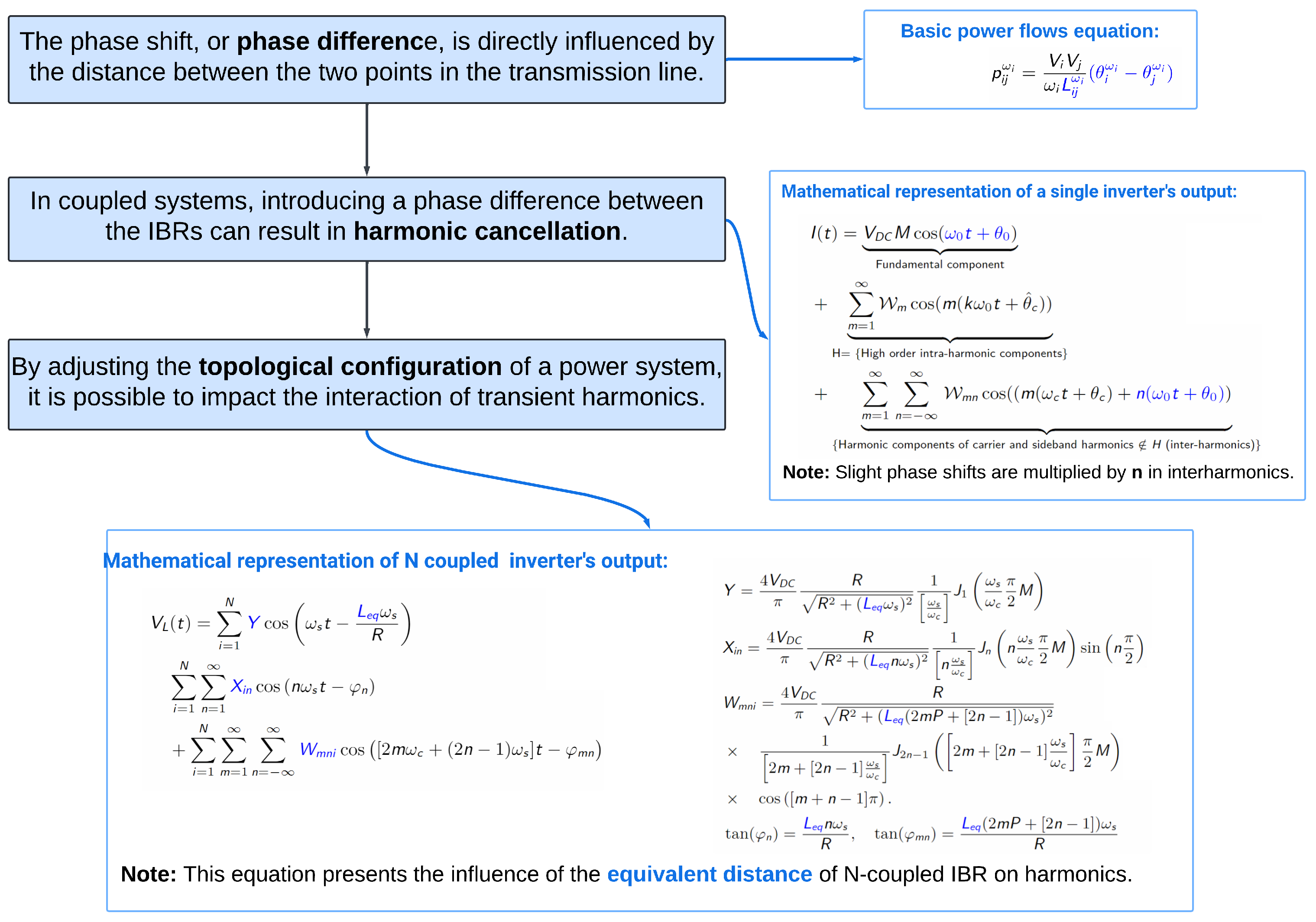
2.1. Explanation of the Relationship between Topological Configuration and Phase in Power Systems Using the Power Flow Equation

To provide a comprehensive explanation of the relationship between topological configuration and phase in power systems, it is essential to elucidate the phase relationship and topology through the basic power flow equation between the two points. The power flow equation for a basic power line can be expressed as Equation (1).

$$p_{ij}^{{\omega }_i}=\frac{V_i{V}_j}{{\omega }_i{L}_{ij}^{{\omega }_i}}({\theta }_i^{{\omega }_i}-{\theta }_j^{{\omega }_i}),$$

(1)

where $p_{ij}$ is the active power output from point i to point j, and ${\omega }_i$ is the average frequency of switching of the inverter. To reflect the influence of operation frequency on this equation, the parameters are defined at ${\omega }_i$ frequency. $L_{ij}^{{\omega }_i}$ is the reactance between point i and point j, ${\theta }_i^{{\omega }_i}$ is the phase angle at point i, and ${\theta }_j^{{\omega }_i}$ is the phase angle at point j at frequency ${\omega }_i$. Also, $V_i$ and $V_j$ are the amplitudes of the voltage of the two points.

At a given frequency and load level, assuming nearly constant voltage, the electrical connection between points is typically characterized by line reactance and phase differences.

In a power network including N buses connected by L power lines, the relationship between net active power (P), nodal voltage magnitude (V), and voltage phase ($\theta$) is governed by Kirchhoff’s circuit laws. It can be written as follows [16]:

$$\begin{array}{cc}\hfill P_m& =V_m\sum _{n=1}^N{V}_n(G_{mn}\cos ({\theta }_m-{\theta }_n)B_{mn}\sin ({\theta }_m-{\theta }_n),\hfill \end{array}$$

(2)

for bus $m=1,2,\dots ,N$. $G_{mn}$ is the magnitude of the real component of the $(m,n)$ element of the bus admittance matrix Y and, B is the the magnitude of imaginary component of it. We can make three assumptions about the system:

(1) Flat voltage profile, i.e., $V_m\approx V_n\approx 1.0$ p.u.;

(2) Approximately homogeneous bus phases across the network, i.e., $\cos ({\theta }_m-{\theta }_n)\approx 1$ and $\sin ({\theta }_m-{\theta }_n)\approx ({\theta }_m-{\theta }_n)$; (because $({\theta }_m-{\theta }_n)$ is near to 0);

(3) The reactive property of a line is much more significant than its resistive property, i.e., $B_{mn}\gg G_{mn}$. Under these assumptions, Equation (2) reduces to the following:

$$\begin{array}{cc}\hfill P_m& =\sum _{n=1}^N{B}_{mn}({\tilde{\theta }}_{mn}),\hfill \end{array}$$

(3)

where $\tilde{\theta }mn$ denotes the approximate system phase angle at the observation point. Considering the above-mentioned assumption and given the fact that $(P_m\gg Q_m)$, it possible to approximate the above expression according to $(P_m\propto I_m^2)$:

$$\begin{array}{cc}\hfill I_m^2& =\sum _{n=1}^N{B}_{mn}^{\prime }({\tilde{\theta }}_{mn}),\hfill \end{array}$$

(4)

where $I_m$ is the net electrical current follow of bus m. For a balanced power system with no active power mismatch, $I_m^2$ is a constant value. In a steady-state system with a constant electrical current fundamental component, a direct relationship between the phase difference and the power network’s topological configuration can be established by examining how the admittance matrix is constructed based on the reactance of power lines.

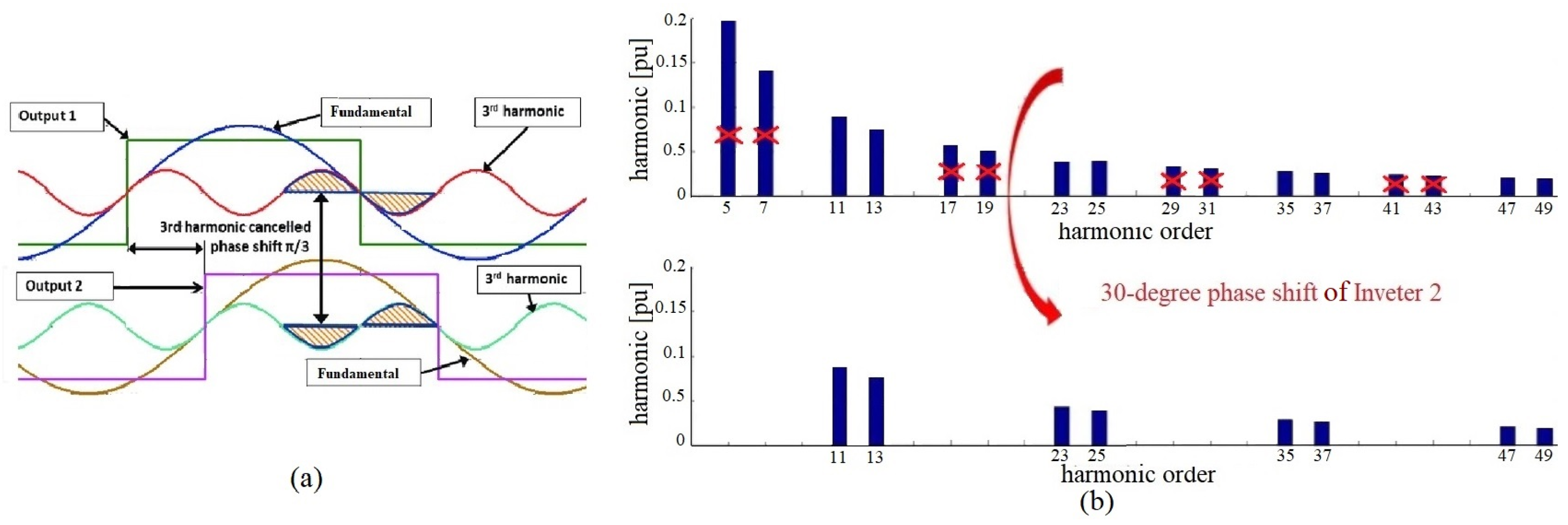
2.2. Exploring the Relationship between Harmonics and Phase

In the preceding subsection, we explicated that by adjusting the reactance, phase difference is induced in power lines. In this section, we aim to elucidate how this phase difference between two lines impacts the harmonics level of the coupled IBR system.

The relationship between harmonics and phase at the interaction point of the coupled system could be explained with the harmonic cancellation effect. The abstract concept of harmonic cancellation involves separating the power supply into two, shifting one source of harmonics 180 degrees to the other, and then combining outputs.

For instance, the output voltage of a full-bridge inverter with a sinusoidal pulse width modulation (SPWM) switching method is mathematically described by equation [15]:

$$\begin{array}{cc}\hfill & V\left(t\right)=\underset{\mathrm{Fundamental}\mathrm{component}}{\underbrace{V_{DC}M\cos ({\omega }_{0}t+{\theta }_0)}},\hfill \\ \hfill & +\underset{\mathrm{H} = \{\mathrm{High}-\mathrm{order}\mathrm{intra}-\mathrm{harmonic}\mathrm{components}\}}{\underbrace{\sum _{m=1}^{\infty }{\mathcal{W}}_m\cos (m(k{\omega }_{0}t+{\widehat{\theta }}_c))}},\hfill \\ \hfill & +\underset{\{\mathrm{Harmonic}\mathrm{components}\mathrm{of}\mathrm{carrier}\mathrm{and}\mathrm{sideband}\mathrm{harmonics} \notin H(\mathrm{inter}-\mathrm{harmonics}\left)\right\},}{\underbrace{\sum _{m=1}^{\infty }\sum _{\begin{array}{c}n=-\infty \end{array}}^{\infty }{\mathcal{W}}_{mn}\cos ((m({\omega }_{c}t+{\theta }_c)+n({\omega }_{0}t+{\theta }_0))}}\hfill \end{array}$$

(5)

where ${\theta }_c$ is the phase of carrier waveform, ${\theta }_0$ is the phase angle of fundamental waveform, and ${\mathcal{W}}_m$ and ${\mathcal{W}}_{mn}$ are magnitudes of intra-harmonics and inter-harmonics, respectively. Without losing generality, ${\widehat{\theta }}_c$ in Equation (5) is the characteristic phase of the inverter carrier of the frequencies that belong to the synchrophasor family of the fundamental frequency where all harmonic components fully commute. $V_{DC}$ is the DC link voltage, $M\in \left[01\right]$ is the modulation index, ${\omega }_c$ is the carrier angular frequency, and ${\omega }_s$ is the fundamental angular frequency. The angular carrier to angular frequency ratio is an integer ($\frac{{\omega }_c}{{\omega }_0}=k$), the carrier and baseband harmonics would be inter-harmonics to the fundamental frequency [15].

When the fundamental component of output electrical voltage shifted by $\Delta \theta$, the term $(n({\omega }_{0}t+{\theta }_0+\Delta \theta ))$, the appropriate phase shifts in inter-harmonics components are multiplied by n. If two identical inverters with similar lines are connected in parallel, there may be a situation where a 180-degree phase shift in one line results in a shift in the harmonic. In this case, there would be two current harmonics with a 180-degree phase difference at the connection point from the two coupled inverters. The corresponding currents would have the same magnitude in the opposite direction, resulting in their cancellation.

Figure 1a shows how a $\pi /6$ degree phase shift in output two results in the third harmonic of two outgoing waves that cancel each other. However, this is not limited to only one harmonic. Figure 1b shows how some of the harmonics are removed with this 30-degree phase shift. The set of these removed harmonics finally determines the impact of phase change on the total harmonic distortion.

This explanation can be extended to the number of inverters. For example, Figure 2 shows N coupled inverters.

A simplified model of N-coupled inverters is used as an example to illustrate the relationship between reactance and harmonics level. This model is based on the unfiltered voltage of an H-bridge and was originally presented in [15]. In this study, the equation is rewritten under the assumption that the inductance of each line may not be equal and that the inverters are identical as follows:

$$\begin{array}{c}{I}_L\left(t\right)=\sum _{i=1}^{N}Y\cos ({\omega }_s\left(t\right)-\frac{L_{eq}{\omega }_s}{R}),\hfill \\ \sum _{i=1}^N\sum _{n=2}^{\infty }{X}_{in}\cos (n{\omega }_s\left(t\right)-{\phi }_n),\hfill \\ +\sum _{i=1}^N\sum _{m=1}^{\infty }\sum _{n=-\infty }^{\infty }{W}_{mni}\cos \left(\begin{array}{c}[2m{\omega }_c+[2n-1]{\omega }_s]\left(t\right)\hfill \\ -{\phi }_{mn}\hfill \end{array}\right),\hfill \\ Y=\frac{4V_{DC}}{\pi }\frac{R}{\sqrt{R^2+{\left(L_{eq}{\omega }_s\right)}^2}}\frac{1}{\left[\frac{{\omega }_s}{{\omega }_c}\right]}{J}_1(\frac{{\omega }_s}{{\omega }_c}\frac{\pi }{2}M),\hfill \\ X_{in}=\frac{4V_{DC}}{\pi }\frac{R}{\sqrt{R^2+{\left(L_{eq}n{\omega }_s\right)}^2}}\frac{1}{\left[n\frac{{\omega }_s}{{\omega }_c}\right]}{J}_n(n\frac{{\omega }_s}{{\omega }_c}\frac{\pi }{2}M)\sin (n\frac{\pi }{2}),\hfill \\ W_{mni}=\frac{4V_{DC}}{\pi }\frac{R}{\sqrt{R^2+{\left(L_{eq}(2mP+[2n-1]){\omega }_s\right)}^2}},\hfill \\ \times \frac{1}{\left[2m+[2n-1]\frac{{\omega }_s}{{\omega }_c}\right]}{J}_{2n-1}(\left[2m+[2n-1]\frac{{\omega }_s}{{\omega }_c}\right]\frac{\pi }{2}M),\hfill \\ \times \cos \left(\right[m+n-1\left]\pi \right),\hfill \\ \tan \left({\phi }_n\right)=\frac{L_{eq}n{\omega }_s}{R},\hfill \\ \tan \left({\phi }_{mn}\right)=\frac{L_{eq}(2mP+[2n-1]){\omega }_s}{R},\hfill \\ L_{eq}=\frac{1}{{\displaystyle \sum _{i=1}^N}\frac{1}{L_i}},\hfill \end{array}$$

(6)

where $V_{DC}$ is the DC link voltage, N is the number of coupled inverters, $M\in \left[01\right]$ is the modulation index, ${\omega }_c$ is the carrier angular frequency, ${\omega }_s$ is the fundamental angular frequency, $J_n\left(x\right)$ is a Bessel function of order n and argument x, m is the carrier index, n is the beseband index, R is the load resistance, $L_{eq}$ is the equivalent inductance, and $P=\frac{f_c}{f_s}$ is the carrier to reference frequency ratio.

Considering $(L_{eq}=1/{\displaystyle \sum _{i=1}^N}\frac{1}{L_i})$, the inductance of all lines determines the equivalent inductance. Therefore, adjusting each power line produces a change in equivalent inductance. As a result, the amplitudes of $X_{in}$ and $W_{mni}$ would be changed. Simultaneously, due to the impact of equivalent inductance in ${\phi }_n$ and ${\phi }_{mn}$, the phases of all harmonic components would be shifted. The impact of changing the equivalent inductance is primarily observed on the higher-order harmonics, as they experience a higher phase shift based on ${\phi }_n$ and ${\phi }_{mn}$ equations. Figure 3 represents a summary of the topics discussed in this section.

Two key characteristics of phase shift and the harmonic cancellation effect on coupled systems, which we aim to illustrate in an experimental setup, could be as follows:

• It does not exert a substantial influence on the fundamental component; however, at higher frequencies, it notably affects the harmonic component.
• The process of harmonic alteration does not follow a linear relationship between harmonic levels and frequency because it may lead to a decrease or increase in harmonic level between two consecutive harmonics orders.

2.3. Terminology and Definitions Used in this Work

2.3.1. Definition of Electrical Distance

The term “electrical distance” carries various definitions depending on the context [18,19]. Generally, it represents the proximity or separation of components within an electrical or power system, forming its topological configuration. In power system analysis, electrical distance describes the effective impedance between network points, considering electrical characteristics such as resistance, capacitance, and inductance that influence energy flow. The definition of electrical distance remains non-unified. It is often defined as the mutual impedance between two points based on their electrical characteristics [20]. Researchers have used this concept in various power system studies to describe the distance between points based on measurements [21,22]. Despite these differing definitions, electrical distance plays a significant role in shaping power system topology. In this study, we adjusted parameters between two points, effectively altering the electrical distance between them and resulting in changes to the topological configuration of the power system.

2.3.2. Relative Distance Ratio

Relative electrical distance refers to the comparison of electrical distances between different points in a power system. Unlike local parameters that describe characteristics at specific locations, relative electrical distance pertains to the system as a whole. It involves assessing the ratio of electrical distances between two points. This comparison helps in understanding the relative impact of electrical distances on various aspects of power system behavior, taking into account the interconnected nature of the entire system.

While local or component parameters focus on the characteristics of individual elements, relative electrical distance looks at the system-level relationship between these elements. It provides valuable insights into how the arrangement and configuration of components affect the overall system performance.

2.3.3. Total Harmonic Distortion (THD)

The level of total harmonic distortion of the electrical voltage is used to comprehensively determine how electrical distance in coupled inverter systems impacts harmonics and is defined as follows:

$$\mathrm{THD}=\sqrt{\sum _{n=2}^N{(\frac{V_n}{V_1})}^2}*100,$$

(7)

where $V_n$ is the magnitude of nth harmonic component, and $V_1$ is the magnitude of fundamental component. In this work, the total harmonic distortion was calculated for the electrical voltage signal.

3. Experiment Design and Primary Findings

3.1. Test Scenarios and Experiment Setup

This subsection introduces the experimental test setup and designed scenario utilized to illustrate the relationship between the topological configuration of the power system and harmonics levels in a power system integrated with IBR.

3.1.1. Design of Test Scenarios

To demonstrate the impact of the topological configuration on the interaction harmonics of the coupled IBR system, a power system was designed with two coupled power lines of IBR clusters, facilitating adjustments to the relative impedance.

A slight mismatch was created between the output of two inverter clusters to instigate the interaction of harmonics. It should be noted that the inverter output is filtered, and the total harmonic distortion (THD) of an individual system is less than 1%. However, the THD increased by over 5% after coupling the two clusters. This change in THD, despite the presence of filters, is attributed to the mismatch between the two clusters. The analyses conducted in this work consider these harmonics, which are termed interaction harmonics. The schematic diagram illustrating the experimental setup for the coupled configuration of IBR clusters is depicted in Figure 4. Here, $\tilde{\theta }mn$ denotes the approximate system phase angle at the observation point, ${\theta }_1$ represents the phase of the output voltage of IBR cluster 1, and ${\theta }_2$ signifies the phase angle of the output of IBR cluster 2. Furthermore, $X_{line1}$, $r_1$, and $c_1$ denote the impedance values of the $\Pi$ model corresponding to line 1, while $X_{line2}$, $r_2$, and $c_2$ signify the impedance values of the $\Pi$ model associated with line 2. Additionally, the capacitance C, resistor R, and inductance L are considered in the coupling interface circuit of two power lines. The study involved ten different test configurations, each at a different characteristic impedance, where the line inductance was adjusted to reflect changes in the electrical distance as well. The inductance of $X_{line1}$ remained constant in all test configurations. In contrast, the inductance of line 2 increased by almost equal amounts with each subsequent test configuration. In the first configuration, the inductance of ${\widehat{X}}_{line2}$ was equal to $X_2$. For the second configuration, an $\Delta X$ and related $\Pi$ model elements were added to ${\widehat{X}}_{line2}$. This approach was repeated for the remaining test configurations, where the inductance value of line 2 increased using the same methodology. Table 2 lists the applied inductance values for each test configuration.

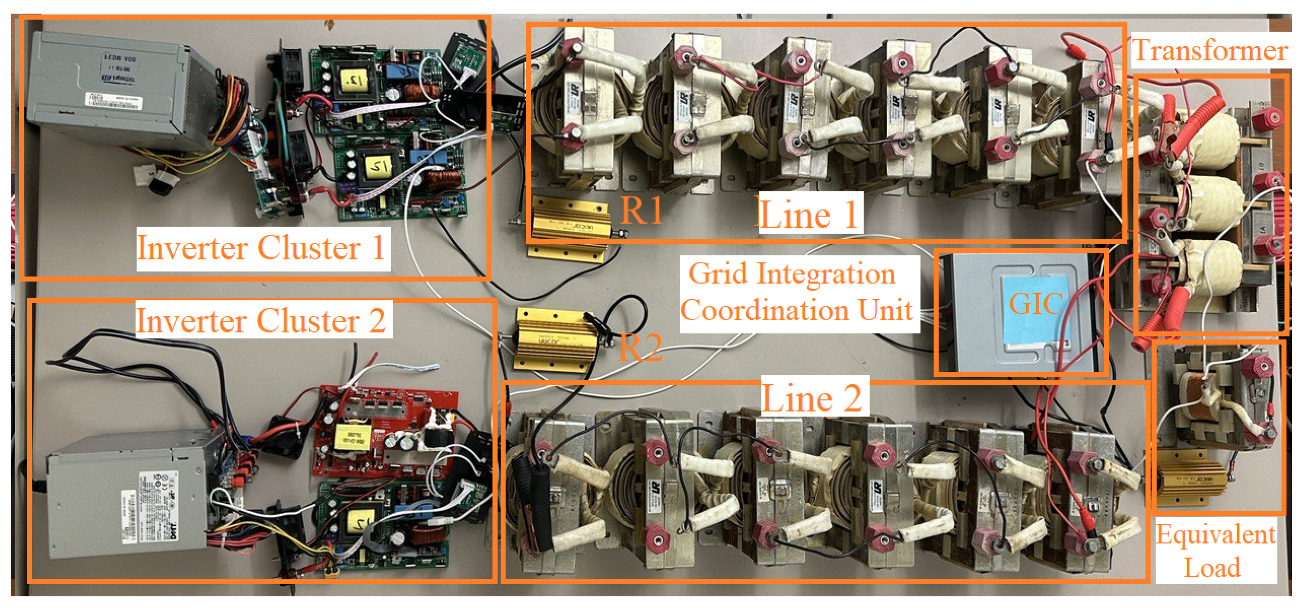
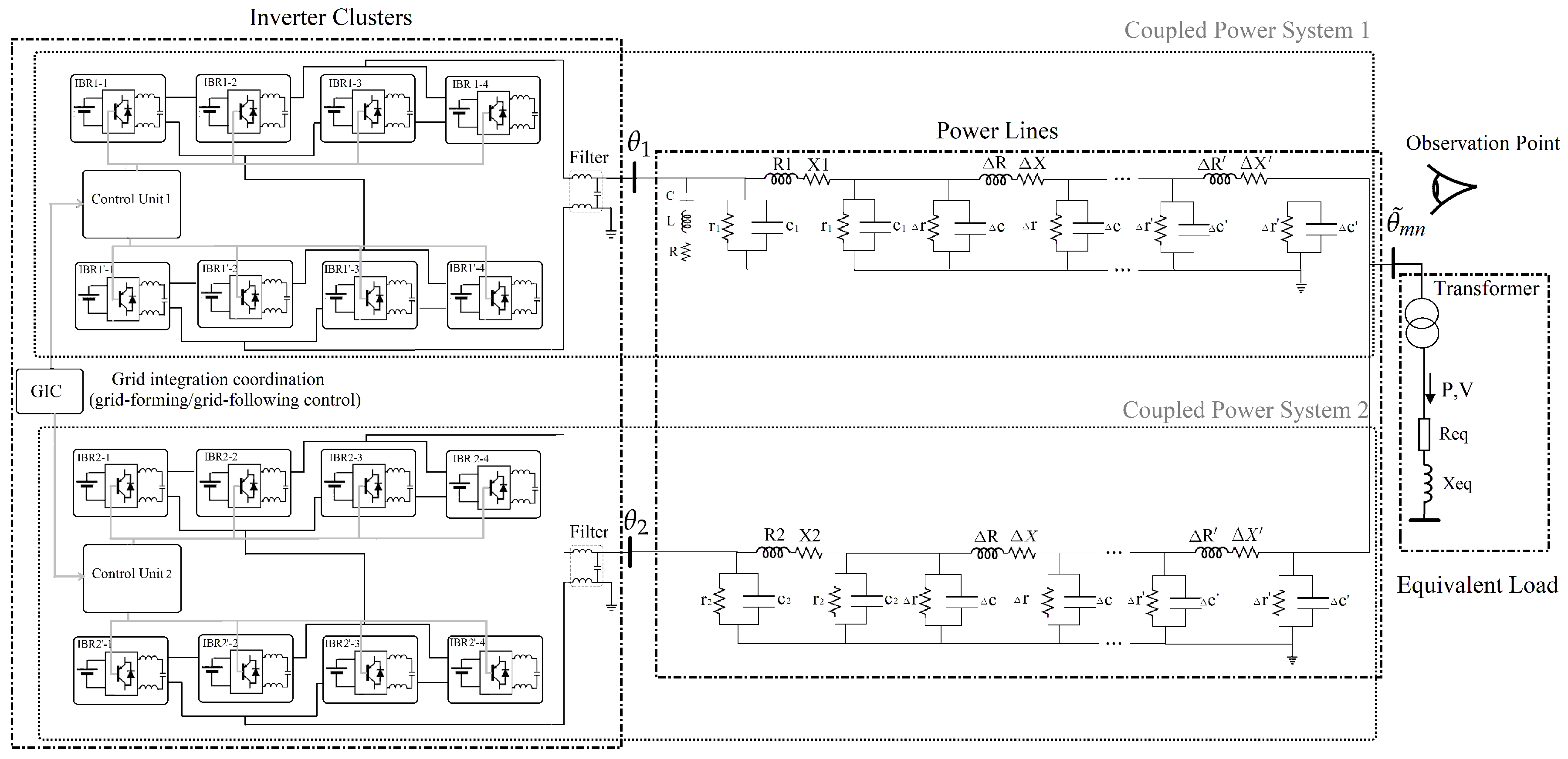
3.1.2. Hardware Configuration of the Experimental Test Setup

Based on the designed test, the hardware configuration included two coupled IBR clusters coordinated within a specific grid integration coordination unit, as illustrated in Figure 5. To set up the power line, a fixed resistance and a series of reactances connected in series were used, allowing for adjustment of the power system’s topological configuration by altering the reactance or electrical distance of power systems.

By setting the reactance of the lines during the tests, the system’s impedance characteristics were changed for various test scenarios. The power line included a sequence of inductances and one resistor. These components were positioned after the IBR clusters. A one-to-one transformer was implemented between lines and equivalent power (P) and voltage (V) load.

Table 2. Parameters used in hardware test setup.

Parameter	Value	Explanation
DC source	12 V	Dc voltage resource
IBR clusters	120 V, 60 Hz, 0.5 kW	Pure sine wave inverters
R1 = R2 = R3	100 $\Omega$	Lines resistance
$R_{eq}$	100 $\Omega$	Equivalent load resistance
$L_{eq}$	0.540 Hz	Equivalent load inductance
Transformer	120 V, 60 Hz	1:1

presents the parameters used in the test setup. In our experimental setup, the test was designed to investigate interaction harmonics, where the mismatch between two coupled systems creates harmonics in the network after the filters on the inverter side. Our objective was not to intentionally increase or decrease reactance in a manner that alters active and reactive power. Extrapolating scaled-down experimental results to full-scale systems with confidence requires careful consideration, especially for nonlinear phenomena like harmonics. Some of the key conditions we tried to satisfy include the following:

• Using representative distribution line parameters and rodding geometries scaled down appropriately;
• Ensuring harmonic sources/loads had comparable behavior to full-scale inverter/rectifier harmonics operating at frequencies high enough that skin-effect scaling is maintained;
• Avoiding excessive thermal transients by using a short test duration.

However, there are inevitably limitations in capturing all performances at full scale.

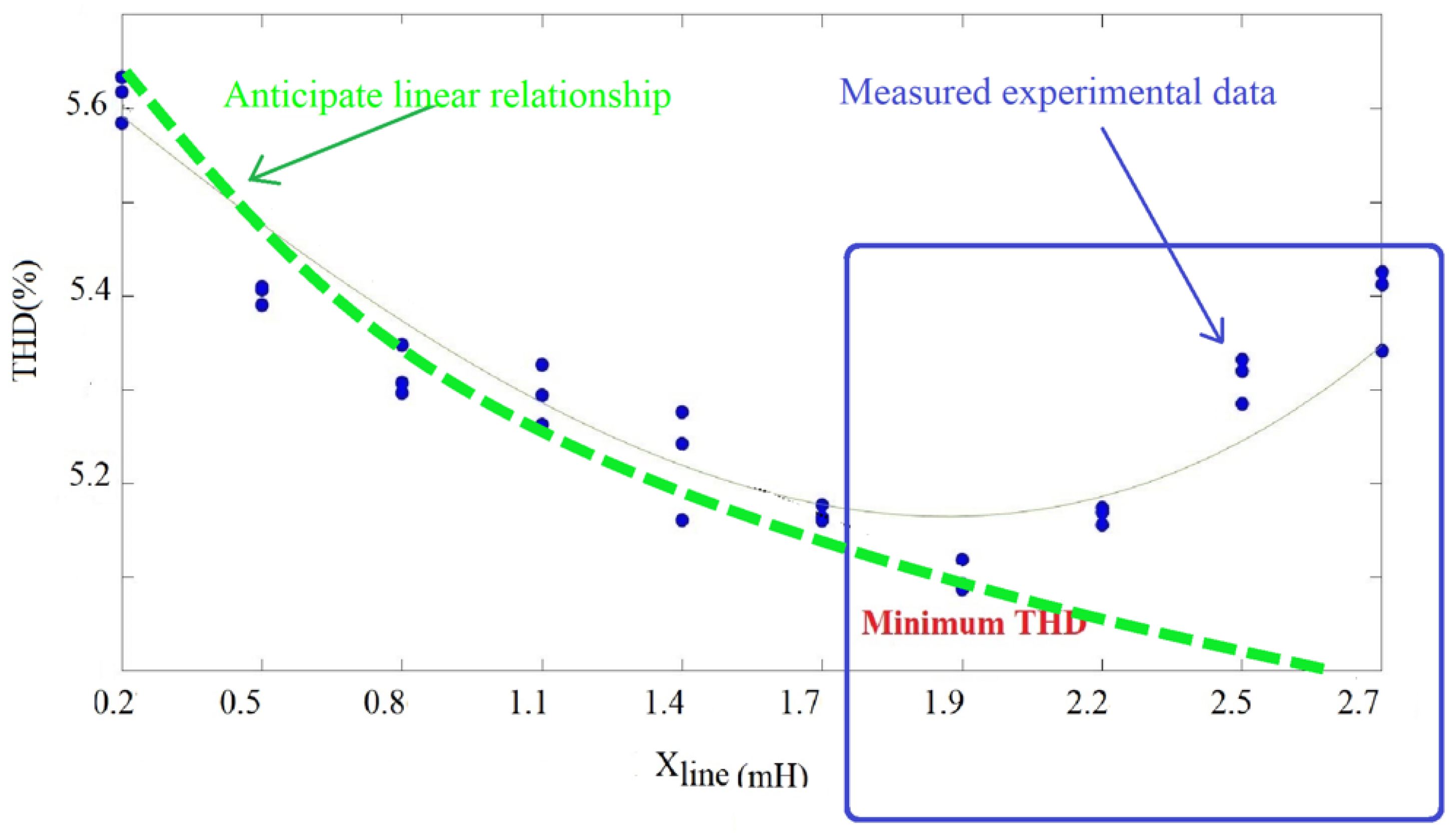
3.2. Demonstration of the Relationship between the Level of Total Harmonic Distortion and the Electrical Distance

The results of this study demonstrate that the change in electrical distance can significantly impact the output total harmonic distortion level in the coupled inverter system. Furthermore, modifying the distance can lead to achieving a minimum output total harmonic distortion level. Figure 6a shows the output voltage waveforms of the ten tested configurations with different inductance values. Each line represents a different configuration, and the x-axis represents time in seconds, while the y-axis represents the configuration number from 1 to 10. The time window of interest is between 0 and 0.04 s. Figure 6b shows the FFT estimations of the same ten configurations in dB, with the x-axis representing frequency in Hz and the z-axis representing the magnitude in dB. The frequency range is limited to 10 kHz. These figures provide a visual representation of the output characteristics of each configuration, which are analyzed in this section.

Figure 7 illustrates the output THD levels of the experimental results at each inductance value (electrical distances), along with a fit curve of output THD level versus electrical distance. Three points for each inductance value represent the results of three repeated tests. The graph clearly shows a decreasing trend of output THD level with increasing electrical distance. However, this trend is reversed after the seventh test configuration position, where ${\widehat{X}}_{line2}$ is 1.989 mH ($X_{line1}=$ 0.280 mH). Contrary to the conventional prescription that THD decreases with increasing electrical distance, this result shows a different trend in that area.

These observations highlight the impact of increasing electrical distance on output THD levels and demonstrate the nonlinear relationship between them. Therefore, appropriate selection of electrical distance can lead to improved current quality in terms of reduced total harmonic distortion and mitigation of relevant harmonics.

4. Further Experimental Investigation Inspired by Analytical Studies

4.1. Design of Test Scenarios

The purpose of further experimental investigation is to examine the topological configuration impact on harmonics by altering the entire structure of the coupled inverter system when the electrical distances of both power lines are changed concurrently as well as the ratio of relative distance (${\widehat{X}}_{line2}/{\widehat{X}}_{line1}$). Figure 8 displays the designed circuit schematic for further investigation. In contrast to the previous experiment, the distances of both lines have been modified in this experimental study. The ratio of the distance of line 2 to line 1 increased in each configuration from 1 to 10. The reactance values used in the lines for each of the 10 configurations are listed in

Table 3. Inductance values in 10 configurations for further investigation (Figure 8).

Test Number	${\widehat{\mathit{X}}}_{\mathit{Line}1}$ (mH)	${\widehat{\mathit{X}}}_{\mathit{Line}2}$ (mH)	Ratio (${\widehat{\mathit{X}}}_{\mathit{Line}2}/{\widehat{\mathit{X}}}_{\mathit{Line}1}$)
1	2.61	0.279	0.10
2	2.253	0.570	0.25
3	1.997	0.864	0.43
4	1.717	1.136	0.66
5	1.436	1.429	0.99
6	1.142	1.708	1.49
7	0.878	1.989	2.26
8	0.574	2.245	3.91
9	0.270	2.580	9.55
10	0.091	2.797	30

.

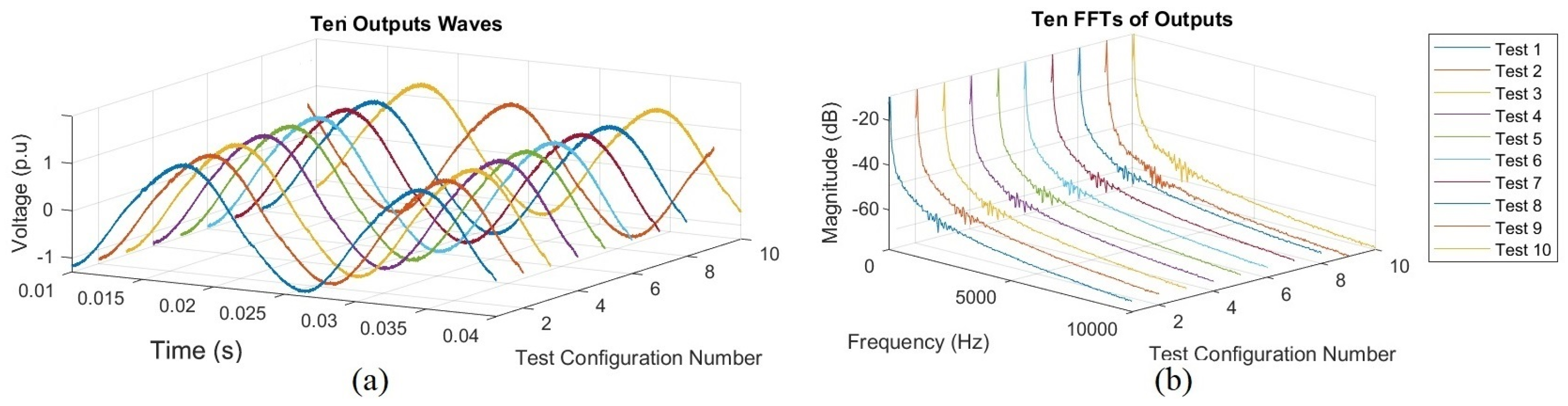
4.2. Further Experimental Results and New Findings

4.2.1. Nonlinear Relationship between Topological Configuration and Harmonics

This section demonstrates that the total level of harmonic distortion is impacted by the entire topological configuration of the power system and is not dependent on just a single line characteristic impedance. Figure 9 illustrates the output THD level versus electrical distance diagram in the experimental test configuration for further investigation, where changes in the distance were applied to both lines. Table 3 lists the inductance values applied to each line for the ten configurations. In comparison to the diagram in Figure 7, the diagram in Figure 9 shows a shift in the point of minimum output THD level. In this experimental setup, where the inductance of line 2 is 1.136 mH, the output THD level is at a minimum value, whereas in the initial experimental setup, it was at 1.989 mH. Moreover, the fit curve of the results shows a sharper decrease in the output THD level versus the electrical distance relationship at the beginning of the graph in the second setup. These differences indicate that changes in the distances of both lines have distinct effects on harmonics and that the total harmonic distortion is affected by the entire structure of the coupled inverter system rather than just a single line.

Also, some other test scenarios have been done, which are presented in

Table 4. Tested scenarios and conclusions.

Sc. No.	Definition of Scenarios	State of Change	Result
1	Increasing the reactance of line 1 while keeping line 2 fixed.	$X_{\mathrm{line}1}$: Fix, $X_{\mathrm{line}2}$: Increase	The nonlinear relationship between output THD and topological configuration changes.
2	Increasing the reactance of line 2 while keeping line 1 fixed.	$X_{\mathrm{line}1}$: Increase, $X_{\mathrm{line}2}$: Fix	Same as in scenario 1: The nonlinear relationship between output THD and topological configuration changes.
3	Simultaneous increase of the reactances of both lines with a constant rate.	$X_{\mathrm{line}1}$: Increase, $X_{\mathrm{line}2}$: Increase	The THD vs. distance curve varies more smoothly with electrical distance compared to the previous two scenarios.
4	Increase in the reactance of line 2, decrease in the reactance of line 1, and a sharp increase in the ratio.	$X_{\mathrm{line}1}$: Increase, $X_{\mathrm{line}2}$: Decrease	The THD vs. distance curve varies more sharply with electrical distance compared to the previous scenarios.

. This finding indicates that the relationship between electrical distance and total harmonics distortion is nonlinear. This nonlinearity highlights the distinct nature of the harmonic relationship with electrical distance compared to the variations arising from passive filters.

In this work, our focus is on adjusting reactance rather than just increasing reactance. By modifying the distances between components or adding/removing IBR lines, we aimed to determine optimal configurations. It is worth noting that optimal configurations were occasionally achieved by reducing or increasing reactance or making adjustments to IBR lines.

4.2.2. Harmonic Cancellation Effect through Self-Compensation

This subsection is focused on a deeper analysis of the analytical explanation in Section 3 and the results discussed in Section 3, which confirms that the variation of total harmonic distortion results from the high-frequency interactions among all coupled IBRs, not the change of IBR outputs by some harmonic control or mitigation technologies. More specifically, changing the electrical distance via phase displacement will cause the cancellation of some harmonics of certain frequencies, which may lead to a reduction in the total harmonics distortion level.

In the analysis of Section 2.1, two key characteristics of harmonic cancellation have been presented. First, the process of harmonic alteration deviates from a nonlinear relationship between harmonic levels and frequency. This nonlinearity may result in either a decrease or increase in harmonic levels between consecutive orders within the combined harmonics produced by coupled inverters. Second, harmonic cancellation minimally impacts both voltage and current fundamental components but significantly influences the harmonic component, particularly at higher frequencies. In the analysis of this section, two key characteristics of harmonic cancellation have been illustrated through the experimental test results.

To illustrate the first characteristic of the harmonic cancellation process, which involves the deviation from a nonlinear relationship between harmonic levels and frequency in the process of harmonic alteration, a radar plot analysis was conducted.

The experimental results obtained in each experiment with different test configurations, from number 1 to 10, were used to plot the radar plot of the harmonics spectrum shown in Figure 10. The radar diagram in Figure 10 shows the magnitude of all individual harmonics in the frequency domain up to 10 kHz for each of the 10 different test configurations. The closer the points are to the center of the circle, the lower the frequency of the harmonic, while the further away the points are from the center, the higher the frequency of the harmonic. The color of each point indicates the magnitude of the harmonic at a certain frequency in dB. Each configuration number corresponds to a specific zone in the radar diagram, which is shown in a clockwise rotation from test configuration 1 to 10. For instance, zone 1 in the radar diagram corresponds to test configuration 1.

By looking at the coordinates of a specific point on the radar diagram, one can determine the test configuration number, frequency, and harmonic level of that particular point. This helps in understanding how changing the distance between coupled IBRs affects the harmonic levels in the frequency domain.

The radar diagram analysis helps to explain the phenomenon of harmonic cancellation and how it affects the output THD level. The electrical distance between IBRs causes a phase shift in the harmonics, which can lead to the cancellation of certain harmonics. The variation in the output THD level is, therefore, the result of the cancellation of these harmonics, and the radar diagram shows that this cancellation effect is not a general trend for all harmonics like the local filtering method, but rather each harmonic has a unique level variation.

For a more precise interpretation of the radar plot, several target points were examined. Tracking some target points at a specific frequency, from the first to the tenth configuration, the color variations of the points (representing the magnitude) are not uniform; they do not decrease or increase at the same time. This implies that each individual harmonic has a distinct relationship with the change in electrical distance. To provide a clearer analysis, Figure 10b illustrates the corresponding harmonic level measured at three target points with 4 kHz, 5 kHz, and 6 kHz frequencies over 10 tested electrical distances. These points are displayed in yellow in zone 1, corresponding to configuration 1 in Figure 10a. By examining the trend of harmonic level changes in these three frequencies, it is apparent that all three harmonics follow a unique trend (Figure 10b). Their increase and decrease do not occur simultaneously, which is significant because it demonstrates that any harmonics with a specific frequency are influenced by a change in electrical distance in a distinct way that corresponds to the harmonic phase change. It indicates that the total harmonic distortion and electrical distance relationship are produced by the combination of these individual changes.

Figure 11a illustrates the fundamental component values obtained for each of the ten test configurations used to investigate the effect of electrical distance changes (the results depicted in this subsection represent a single repetition of the test results presented in Section 3.2, Table 2, and Figure 7). Our goal is to demonstrate that the correlation between THD levels and electrical distance is not solely due to changes in the fundamental values of line voltage. The results indicate that the percentage of changes in fundamental components is relatively small, which could be attributed to measurement accuracy. The maximum difference observed from the 120 V voltage level is 1.8 V. The difference between the highest and lowest values is less than 2% of the minimum value, whereas the THD level difference is 10%. Moreover, Figure 11b illustrates that there is no linear correlation between the patterns of change of the fundamental components in the ten test configurations and the THD level variation. This means that there are other factors, in addition to changes in the fundamental values of line voltage, that contribute to the correlation between THD levels and electrical distance. Also, this relatively small change in fundamental component values may not have a significant impact on the correlation between THD levels and electrical distance.

5. Concluding Remarks

The power grid has traditionally been regarded as a large low-pass power filter, with its system-level impact on harmonic propagation over the power lines viewed as a linear or first-order effect. The novel aspect of how the topological configuration influences the level of harmonics accompanying the energy flow in the power grid, primarily driven by coupled inverter-based energy resources, advances our understanding of the relationship between the power grid structure and harmonics.

If we represent the structural impact of the grid configuration with the underlying characteristic impedance of a cluster of IBRs and express the relative distance between different IBR clusters through the ratio of characteristic impedance ratios, we experimentally discovered that the impact of the coupling configuration of IBR clusters on the level of power flow harmonics, as indicated by the total harmonic distortion index, is nonlinear. As illustrated in Figure 7 and Figure 9 for the two IBR cluster setup, the total harmonic level initially decreases with an increase in the relative distance ratio. However, as we further increase the ratio, the level of harmonics surprisingly begins to increase significantly.

Hundreds of intensive experiments with different configurations, line impedances, IBRs, and load levels have been carried out in this way, and every one of them showed the effect to a greater or lesser degree. These experiments also confirm that this nonlinearity is associated with the grid structure, as a proportional increase in characteristic impedances among the IBR clusters has a minor impact on the harmonics. In other words, it is the structural configuration, represented by the characteristic impedance ratio, that causes this nonlinear effect.

This discovery suggests a potential new approach to limiting the penetration of complex IBR harmonics in the power grid from a system-wide perspective. This approach is distinct from conventional component-level or localized solutions employed today, such as inverter control, power filtering, and transformer tap changes. It is particularly attractive because increasing the capacity of power filters significantly raises costs and may introduce other complex effects like electromagnetic resonance. It is worth mentioning that reducing the level of power flow harmonics through an appropriate reconfiguration of the coupling structure is a cost-effective, independent option. This approach leverages the self-compensation interactions of IBR clusters without altering the active power flow, making it an attractive alternative.

References

1. Gu, Y.; Green, T.C. Power System Stability with a High Penetration of Inverter-Based Resources. Proc. IEEE 2023, 111, 832–853. [Google Scholar] [CrossRef]
2. Hoke, A.; Gevorgian, V.; Shah, S.; Koralewicz, P.; Kenyon, R.W.; Kroposki, B. Island power systems with high levels of inverter-based resources: Stability and reliability challenges. IEEE Electrific. Mag. 2021, 9, 74–91. [Google Scholar] [CrossRef]
3. Matevosyan, J.; MacDowell, J.; Miller, N.; Badrzadeh, B.; Ramasubramanian, D.; Isaacs, A.; Quint, R.; Quitmann, E.; Pfeiffer, R.; Urdal, H.; et al. A future with inverter-based resources: Finding strength from traditional weakness. IEEE Power Energy Mag. 2021, 19, 18–28. [Google Scholar] [CrossRef]
4. Leon, J.I.; Kouro, S.; Franquelo, L.G.; Rodriguez, J.; Wu, B. The essential role and the continuous evolution of modulation techniques for voltage-source inverters in the past, present, and future power electronics. IEEE Trans. Ind. Electron. 2016, 63, 2688–2701. [Google Scholar] [CrossRef]
5. Impram, S.; Nese, S.V.; Oral, B. Challenges of Renewable Energy Penetration on Power System Flexibility: A Survey. Energy Strategy Rev. 2020, 31, 100539. [Google Scholar] [CrossRef]
6. Zhang, Y.; Roes, M.; Hendrix, M.; Duarte, J. Symmetric-component decoupled control of grid-connected inverters for voltage unbalance correction and harmonic compensation. Int. J. Elect. Power Energy Syst. 2020, 115, 105490. [Google Scholar] [CrossRef]
7. Tariq, M.; Upadhyay, D.; Khan, S.A.; Alhosaini, W.; Peltoniemi, P.; Sarwar, A. Novel Integrated NLC-SHE Control Applied in Cascaded Nine-Level H-Bridge Multilevel Inverter and Its Experimental Validation. IEEE Access 2023, 11, 22209–22220. [Google Scholar] [CrossRef]
8. Muhammad, T.; Khan, A.U.; Abid, Y.; Khan, M.H.; Ullah, N.; Blazek, V.; Prokop, L.; Misák, S. An Adaptive Hybrid Control of Reduced Switch Multilevel Grid Connected Inverter for Weak Grid Applications. IEEE Access 2023, 11, 28103–28118. [Google Scholar] [CrossRef]
9. Koiwa, K.; Takahashi, H.; Zanma, T.; Liu, K.-Z.; Natori, K.; Sato, Y. A Novel Filter With High Harmonics Attenuation and Small Dimension for Grid-Connected Inverter. IEEE Trans. Power Electron. 2023, 38, 2202–2214. [Google Scholar] [CrossRef]
10. Hu, H.; Shi, Q.; He, Z.; He, J.; Gao, S. Potential harmonic resonance impacts of PV inverter filters on distribution systems. IEEE Trans. Sustain. Energy 2015, 6, 151–161. [Google Scholar] [CrossRef]
11. Nduka, O.S.; Pal, B.C. Harmonic domain modeling of PV system for the assessment of grid integration impact. IEEE Trans. Sustain. Energy 2017, 8, 1154–1165. [Google Scholar] [CrossRef]
12. Baburajan, S.; Wang, H.; Kumar, D.; Wang, Q.; Blaabjerg, F. DClink current harmonic mitigation via phase-shifting of carrier waves in paralleled inverter systems. Energies 2021, 14, 4229. [Google Scholar] [CrossRef]
13. Moeini, A.; Wang, S.; Zhang, B.; Yang, L. A Hybrid Phase Shift-Pulsewidth Modulation and Asymmetric Selective Harmonic Current Mitigation-Pulsewidth Modulation Technique to Reduce Harmonics and Inductance of Single-Phase Grid-Tied Cascaded Multilevel Converters. IEEE Trans. Ind. Electron. 2020, 67, 10388–10398. [Google Scholar] [CrossRef]
14. Du, L.; He, J. A Simple Autonomous Phase-Shifting PWM Approach for Series-Connected Multi-Converter Harmonic Mitigation. IEEE Trans. Power Electron. 2019, 34, 11516–11520. [Google Scholar] [CrossRef]
15. Hemmati, R.; Kandezy, R.S.; Safarishaal, M.; Zoghi, M.; Jiang, J.N.; Wu, D. Impact of Phase Displacement among Coupled Inverters on Harmonic Distortion in MicroGrids. In Proceedings of the 2023 IEEE Transportation Electrification Conference Expo (ITEC), Detroit, MI, USA, 21 June 2023; pp. 1–6. [Google Scholar]
16. Albadi, M. Power Flow Analysis. In Computational Models in Engineering; Intechopen: London, UK, 2020; pp. 11–13. [Google Scholar]
17. Tyshko, A. Sequential Selective Harmonic Elimination and Outphasing Amplitude Control for the Modular Multilevel Converters Operating with the Fundamental Frequency. In Power System Harmonics—Analysis, Effects and Mitigation Solutions for Power Quality Improvement; Intechopen: London, UK, 2018; pp. 14–30. [Google Scholar]
18. Mao, X.; Zhu, W.; Wu, L.; Zhou, B. Comparative study on methods for computing electrical distance. Int. J. Electr. Power Energy Syst. 2021, 130, 106923. [Google Scholar] [CrossRef]
19. Poudel, S.; Ni, Z.; Sun, W. Electrical distance approach for searching vulnerable branches during contingencies. IEEE Trans Smart Grid. 2018, 9, 3373–3382. [Google Scholar] [CrossRef]
20. Aghamohammadi, M.R.; Mahdavizadeh, S.F.; Rafiee, Z. Controlled Islanding Based on the Coherency of Generators and Minimum Electrical Distance. IEEE Access 2021, 9, 146830–146840. [Google Scholar] [CrossRef]
21. Peng, P.; Chen, K.; Xu, T.; Li, C. A calculation method of electrical distance considering operation mode. J. Phys. Conf. Ser. 2019, 1176, 062018. [Google Scholar] [CrossRef]
22. Fang, G.J.; Bao, H. A Calculation Method of Electric Distance and Subarea Division Application Based on Transmission Impedance. IOP Conf. Ser. Earth Environ. Sci. 2017, 104, 012006. [Google Scholar] [CrossRef]
Figure 1. (a) Third harmonic cancellation through a 60-degree phase shift of inverter 2 in a two-coupled inverter system. (b) Harmonic cancellation through a 30-degree phase shift of inverter 2 in a two-coupled inverter system [17].
Energies 17 02512 g001
Figure 2. Topological configuration of N coupled inverters.
Energies 17 02512 g002
Figure 3. Summary of the discussed topics regarding the relationship between topological configuration and harmonics level).
Energies 17 02512 g003
Figure 4. Schematic of the initial experimental setup: exploring 10 test configurations, where X ^ l i n e 2 is altered but X l i n e 1 remains the same (Table 1).
Energies 17 02512 g004
Figure 5. The hardware configuration of the experimental test setup.
Energies 17 02512 g005
Figure 6. Experimental results of the impact of electrical distance on total harmonic distortion in coupled inverter systems. (a) Voltage waveform of ten tested configurations with varying inductance. (b) Fast Fourier transform (FFT) analysis of ten tested configurations showing the levels of harmonic distortion (dB).
Energies 17 02512 g006
Figure 7. Experimental result of output THD level vs. electrical distance for initial experimental study (test repeated 3 times at any distance).
Energies 17 02512 g007
Figure 8. Schematic of the extended experimental setup: incorporating 10 test configurations (Figure 4); both X ^ l i n e 1 and X ^ l i n e 2 have been changed (Table 3).
Energies 17 02512 g008
Figure 9. Experimental result of output THD level vs. electrical distance for further investigation (ratio = X ^ l i n e 2 / X ^ l i n e 1 ).
Energies 17 02512 g009
Figure 10. (a) Radar diagram of frequencies of output experimental results in Section 2, showing the harmonic content of the inverter-based power system with two coupled inverter systems. (b) The magnitude of harmonics at 4 kHz, 5 kHz, and 6 kHz frequencies is represented in dB (the results depicted in this figure represent a single repetition of the test results presented in Section 3.2, Table 2, and Figure 7).
Energies 17 02512 g010
Figure 11. Experimental results show the change of fundamental component values through test 1–10 (the results depicted in this figure represent a single repetition of the test results presented in Section 3.2, Table 2, and Figure 7) (a) Fundamental component values across ten test configurations; (b) relationship between THD and fundamental component values. (The x-axis shows increasing fundamental component values).
Energies 17 02512 g011