Abstract
The non-technical losses caused by abnormal power consumption behavior of power users seriously affect the revenue of power companies and the quality of power supply. To assist electric power companies in improving the efficiency of power consumption audit and regulating the power consumption behavior of users, this paper proposes a power consumption anomaly detection method named High-LowDAAE (Autoencoder model for dual adversarial training of high low-level temporal features). High-LowDAAE adds an extra “discriminator” named AE3 to USAD (UnSupervised Anomaly Detection on Multivariate Time Series), which performs the same function as AE2 in USAD. AE3 performs the same function as AE2 in USAD, i.e., it is trained against AE1 to enhance its ability to reconstruct average data. However, AE3 differs from AE2 because the two “discriminators” correspond to the high-level and low-level time series features output from the shared encoder network. By utilizing different levels of temporal features to reconstruct the data and conducting adversarial training, AE1 can reconstruct the time-series data more efficiently, thus improving the accuracy of detecting abnormal electricity usage. In addition, to enhance the model’s feature extraction ability for time-series data, the self-encoder is constructed with a long short-term memory (LSTM) network, and the fully connected layer in the USAD model is no longer used. This modification improves the extraction of temporal features and provides richer hidden features for the adversarial training of the dual “discriminators”. Finally, the ablation and comparison experiments are conducted using accurate electricity consumption data from users, and the results show that the proposed method has higher accuracy.
1. Introduction
1.1. Research Significance
In recent years, with the rise and popularization of the “Smart Grid”, more and more attention has been paid to the transmission and distribution losses in its operation, which can be broadly classified into two categories: technical losses and non-technical losses. Among them, the serious non-technical losses, i.e., abnormal power consumption behavior of customers. Abnormal power consumption behavior not only affects the revenue of power supply companies, but also constitutes an obstacle to the development of the smart grid [1]. The economic source of power supply companies mainly relies on the sale of electricity, and these revenues are in turn used for the construction of power stations, transmission lines, power supply equipment, and the operation of power grids in order to maintain the stable operation of the power industry and promote its further development [2]. The goal of smart grids is to improve resource utilization, ensure safe and stable operation of the grid, reduce transmission losses, and reduce environmental impact by analyzing, utilizing, and making decisions on electricity consumption data collected from meter terminals [3,4]. However, abnormal power consumption behaviors, mainly power theft, have seriously damaged the interests of power supply companies, disrupted the order of power consumption in the market, and affected the stable operation of power grids. Abnormal power consumption behavior increases line loss and brings a huge burden to power supply companies. Moreover, most of the electricity stealing behaviors are achieved by pulling wires privately and changing the internal metering method of power meters to pay less for electricity, which not only damages the basic power facilities, but also seriously threatens the safe and stable operation of the power grid. Electricity itself is a high-risk product, as electricity theft behavior has great security risks: it easy to cause fires, threatening people’s personal and property safety, and bringing instability to social harmony. According to statistics, in recent years, fire accidents and electrocution casualties caused by power theft reached 40%; the consequences are very serious [5]. In view of this, it is especially critical to develop accurate and efficient methods for detecting abnormal power usage.
As far as data types are concerned, the detection of abnormal power usage behavior involves time-series data, which consists of sequential values that vary over time, and these sequential values truly record the key information of the system at various points in time [6], thus abnormal power usage behavior detection can be regarded as an anomaly detection (AD) problem regarding time-series data. The core objective of anomaly detection, also known as outlier detection, is to identify individuals whose behavior or patterns differ significantly from normal behavior or patterns [7]. In numerous studies in data mining, outliers are often treated as noise and not emphasized. However, in numerous application domains, such as fraud detection [8], process monitoring [9], and the detection of abnormal electricity behavior explored in this paper, discovering those outliers that belong to a small number of categories may be more critical than identifying the regular ones. In these scenarios, the detection of anomalous samples is a key component in identifying potential safety hazards, performance issues, or faulty equipment.
1.2. Related Work
In recent years, the application of data mining in abnormal behavior recognition is mainly divided into unsupervised learning and supervised learning. The commonly used algorithms in unsupervised learning include clustering analysis and outlier detection. Ref. [10] improves the C-mean clustering algorithm by introducing a fuzzy classification matrix, and considers the one with the largest normalized metric distance as the abnormal behavior of electricity consumption. Ref. [11] improves the outlier detection algorithm by means of a Gaussian kernel function and identifies the outliers of electricity consumption data of electricity users. Ref. [12] is the recognition of abnormal [12] in the identification of abnormal power usage behavior. Firstly, the load sequence of the power users is mapped to the two-dimensional plane, then the local outlier factor (LOF) algorithm is improved based on the grid processing technique, and finally, the degree of outlier of each individual power user is calculated to identify the abnormal power usage behaviors among them. Supervised learning views abnormal power usage identification as a binary classification problem, which divides power users into normal and abnormal users. Ref. [13] proposed a random forest (RF) classification algorithm improved by random weight network and distributed computation based on Hadoop, which achieves satisfactory results in abnormal power usage identification. Ref. [14] proposed a random forest (RF) classification algorithm based on support vector machine (SVM) and distributed computation based on Hadoop. Support Vector Machine (SVM) for abnormal power usage behavior detection. Ref. [15] proposed an Extreme Gradient Boosting (XGBoost)-based power theft detection method and introduced a genetic optimization algorithm for feature selection, which effectively improves the power theft detection accuracy. Traditional clustering methods in unsupervised learning have a strong dependence on parameters, while the selection of parameters increases the complexity of the algorithm. In addition, due to the large uncertainty in the distribution of power user data, the selection of the threshold value has a great impact on the recognition accuracy. Most of the classification methods based on supervised learning need to rely on manual work to extract the trend, series standard deviation, slope and other characteristics of electricity consumption data before performing the classification task, which makes the preliminary work more complicated [16]. Moreover, due to the high cost of expert annotation and the impossibility of ensuring that all anomaly types can be recognized, it is particularly important to design models that do not rely excessively on annotated data. Therefore, a more reliable method is needed to accurately identify abnormal power usage behavior.
Deep learning, as a cutting-edge field of machine learning, is essentially a deep network architecture that contains multiple hidden layers. Deep learning algorithms do not need to carry out manual feature extraction in the early stage, and can automatically extract a large number of representative feature information by virtue of its powerful multilayer nonlinear mapping capability, and can autonomously learn feature attributes according to the training samples, which provides a solution to the problem of subjectively setting thresholds and the difficulty of manually extracting features in the traditional method of identifying abnormal power usage behavior [17]. In addition, deep learning methods can take full advantage of the massive electricity consumption data under the interference of noisy data and mine the potential correlations inherent in the data. All of the above advantages motivate deep learning algorithms to be applied in the field of abnormal electricity consumption behavior recognition.
Unsupervised deep learning-based anomaly detection techniques utilize the powerful linear and nonlinear modeling capabilities of deep learning to learn hierarchical feature distinctions from complex data [18]. Among many deep learning methods, generative modeling anomaly detection methods represented by autoencoder (AE) and generative adversarial network (GAN) are the current research hotspots in academia [19]. An autoencoder consists of an encoder and a decoder, which are responsible for extracting features of the input data in the latent space and giving low-dimensional representations of these features; while the decoder upscales these low-dimensional representations to reconstruct the input data [20]. During the encoding process, noise and disturbing information in the data is suppressed, allowing the encoder to obtain a better representation of the features of the normal data. Through the action of decoder, the autoencoder is able to reconstruct the normal data with a higher degree of reproduction, while a large reconstruction error is generated for the abnormal data. Ref. [21] used the reconstruction error of the autoencoder as the anomaly score, and based on the magnitude of the anomaly score, it realized the detection of the abnormal electricity usage behavior. The GAN-based anomaly detection method was first proposed when it was used for anomaly detection in medical images, which aroused extensive attention from scholars on the application of GAN in the field of anomaly detection [22]. The original GAN determines anomalies by comparing the distributional differences between the original data and the generated data, which results in a model that requires a large amount of computational resources, and the GAN suffers from the problem of pattern collapse and is relatively difficult to train. Despite the wide application of GAN in anomaly detection, the research on anomaly detection of time series is still relatively small. In order to improve the training speed of the detection model, Ref. [23] proposed an unsupervised anomaly detection model (USAD) with fewer parameters, which consists of two autoencoders sharing the encoder, and amplifies the reconstruction error of anomalous data through adversarial training, and demonstrates a better detection performance, but there is only one “discriminator”. It is difficult to provide accurate feedback on both global and local features. OmniAnomaly is a stochastic recurrent neural network model that combines GRU and VAE. This model learns the normal patterns of multivariate time-series data and identifies anomalies using reconstruction probabilities. The encoder part of LSTM-VAE consists of LSTM units, and like typical encoders in VAE architecture, it generates a two-dimensional output that is used to approximate the mean and variance of potential distributions. The decoder samples from a two-dimensional latent distribution to form a three-dimensional time series. Next, the generated time series is reconnected with the original classification embedding sequence through LSTM units to reconstruct the original data sequence. Finally, anomalies are detected based on reconstruction errors and discrimination results. Both models improve their detection accuracy by enhancing their ability to extract features from temporal data. The MAD-GAN model adopts a stacked LSTM network with a depth of 3 and containing 100 hidden (internal) units. Its discriminator is a relatively simple LSTM network with a depth of 1 and also has 100 hidden units, used to support the reconstruction of multivariate time series. The advantages and disadvantages of these deep-learning-based anomaly detection algorithms are shown in Table 1.

Table 1.
Introduction to Deep Learning Methods.
Currently, the research on unsupervised methods based on the detection of electricity theft is carried out independently in feature extraction and anomaly detection, while the actual load sequence has a complex pattern, and the existing methods for extracting time period features are only applicable to the detection of electricity theft that conforms to the assumption of basic smoothness of electricity consumption by normal users, and when the data does not conform to the above mentioned situation, the feature extraction methods will be ineffective [24]. In addition, the presence of noise and complex anomaly patterns in load sequences makes it more difficult to capture highly complex temporal correlations. When extracting features of users’ long-term electricity use, the detection effect will also deteriorate if the selected time duration is inappropriate, leading to the low applicability of unsupervised methods for electricity theft detection.
Aiming at the above problems, this paper adopts the deep learning model of unsupervised learning, improves the USAD model for the characteristics of time-series data, and proposes an autoencoder model with dual adversarial training of high and low-level spatio-temporal features. The model adds an extra “discriminator” on top of USAD, which aims to further strengthen the data reconstruction ability of AE1 in USAD. At the same time, an LSTM network is introduced as the self-encoder structure, which can provide different levels of temporal features for the two “discriminators”, thus enhancing the model’s ability to capture complex temporal correlations in temporal data. This approach can effectively cope with different patterns of anomalous power consumption data and significantly improve the accuracy of the model in detecting anomalous behaviors.
2. Detection of Abnormal Electricity Consumption Behavior Based on High-LowDAAE
2.1. Problem Definition
With the continuous development of smart distribution networks and measurement systems, the power data of distribution networks are gradually characterized by large data volume, multiple types and rapid growth. However, affected by factors such as equipment failures, communication failures, and power grid fluctuations, these data contain a large amount of abnormal power data. Therefore, from the perspective of the power supply company, not only is it necessary to improve the performance of the smart meter itself in resisting physical attacks, but it should also further establish a power theft detection system based on the existing power metering automation system, and make full use of the data provided by the Advanced Measurement Instrumentation (AMI) system to build a model for detecting abnormal power usage in the station area, in order to safeguard the safe and stable operation of the power system.
Abnormal electricity behavior detection is essentially a binary classification problem, which requires the design of a corresponding detection method to distinguish between normal and abnormal electricity behavior, and to calculate the classification accuracy based on the evaluation index. In this paper, a High-LowDAAE model for abnormal power usage behavior detection is proposed based on the unsupervised deep learning idea, and the proposed method is described in detail in the following.
2.2. Proposed Method
2.2.1. USAD Model
AE is an unsupervised artificial neural network consisting of an encoder E and a decoder D. The encoder partially maps the input X to a set of latent variables Z, while the decoder maps the latent variables Z back to the input space as a reconstruction R. The difference between the original input vector X and the reconstruction R is called the reconstruction error. Therefore, the training objective aims to minimize this error. The definition is as follows:
An autoencoder (AE) is an unsupervised learning artificial neural network that consists of two parts: an encoder E and a decoder D. The encoder E is the encoder and the decoder D is the decoder. The encoder E is responsible for converting the input data X into a set of latent variables Z, while the decoder D reconstructs these latent variables Z back into the input space to form the reconstructed data R. The difference between the input data X and the reconstructed data R is called the reconstruction error. Therefore, the core objective of training an autoencoder is to minimize this reconstruction error. Specifically, it can be defined as follows:
where , , denotes L2 regularization.
For the anomaly detection method, an autoencoder (AE) model is utilized to assess the degree of abnormality of the data through the reconstruction error, in which the data points with large reconstruction errors are judged as abnormal. During the training process, the model is only exposed to normal data samples, so the AE is effective in reconstructing normal data in the inference phase, but is not effective in reconstructing anomalous data that is not encountered during the training process. However, when the abnormal data is very similar to the normal data, i.e., the degree of abnormality is mild, the reconstruction error may not be significant, resulting in failure of abnormality detection. This is because the design goal of AE is to reconstruct the input data as close as possible to the distribution of normal data. To solve this problem, the AE needs to have the ability to recognize anomalies in the input data and reconstruct them efficiently based on this.
GAN, or Generative Adversarial Network, is an unsupervised learning neural network architecture that is based on the principle of a very small, very large game between two competing networks, which are trained simultaneously. One network acts as a generator (G), whose goal is to generate realistic data, and the other network acts as a discriminator (D), whose task is to distinguish between the real data and the data generated by generator G. The training objective of the generator G is to maximize the probability that the discriminator D makes an error, while the training objective of the discriminator D is to minimize its classification error. Similar to the autoencoder (AE)-based anomaly detection method, the GAN-based anomaly detection is also trained using normal data. After training, discriminator D is used as an anomaly detector. If the distribution of the input data does not match the distribution of the data learned during training, the discriminator D assumes that these data come from the generator G and marks them as anomalous. However, the training process of GANs is not always stable and smooth due to problems such as pattern collapse and training non-convergence, which is usually caused by the imbalance of capabilities between the generator and the discriminator.
In view of the above problems, a two-stage adversarial training autoencoder architecture, the USAD model, is proposed. On the one hand, the USAD model overcomes the intrinsic limitations of autoencoders (AEs) by training a model that can recognize whether the input data contains anomalous data or not, as a way to achieve more efficient data reconstruction. On the other hand, the AE architecture is able to gain stability during adversarial training, and therefore also solves the problem of pattern collapse and non-convergence often encountered in Generative Adversarial Networks (GANs).
As shown in Figure 1, the USAD model consists of three parts: an encoder network E and two decoder networks D1 and D2. These three parts form two autoencoders AE1 and AE2, which share the same encoder network:
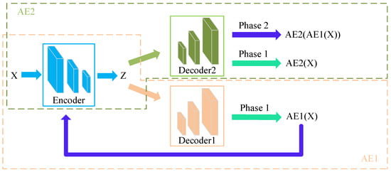
Figure 1.
USAD model training architecture.
The architecture shown in Equation (2) utilizes a two-stage training approach. In the first stage, two autoencoders (AEs) are trained to learn how to reconstruct normal input data. Then, in the second stage, the two AEs learn by adversarial training, where AE1 tries to “confuse” AE2, while AE2 acts as a “discriminator” to distinguish whether the data is real (directly from the input data) or reconstructed by AE1. or reconstructed by AE1.
Phase 1: Autoencoder training. In the first stage, the goal is to train each AE to reconstruct the input. The input data X is compressed into the potential space Z by the encoder E and then reconstructed by each decoder. According to Equation (1), the training objective is:
Phase 2: Adversarial training. In the second phase of adversarial training, the goal is to train AE2 to be able to distinguish between the data reconstructed by AE1 and the original real data, and at the same time to train AE1 to “confuse” AE2. The data from AE1 is compressed again into the potential space and then reconstructed by AE2. During adversarial training, the goal of AE1 is to minimize the difference between its output and the output of AE2, while the goal of AE2 is to maximize the difference; AE1 tries to “confuse” AE2 into believing that the reconstructed data is real, while AE2 tries to distinguish the reconstructed candidate data of AE1 from the real data. The goal of training can be stated as follows:
Are expressed as follows:
Then, the two-stage Loss is combined as follows:
where denotes a training period.
As shown in Figure 2, the USAD model enters the detection phase after the offline training is completed. In the detection phase, firstly, the data is compressed into the hidden variable Z through the coding layer, then, the hidden variable Z goes through the decoder 1 to obtain the reconstructed output , and at the same time, the is again re-passed through the coding layer to be compressed into the hidden variable, and then it passes through the decoder 2 to obtain the reconstructed output , and the weighted sum of the two reconstruction outputs in terms of the reconstruction error relative to the input data is defined as the anomaly score:
where is used to parameterize the trade-off between FP (False Positive) and TP (True Positive). If , then the amount of TP and FP is decreased. Conversely, if , the amount of both TP and FP is increased. The USAD model will represent high detection sensitivity scenarios and indicate low inspection sensitivity scenarios. This parameterization scheme has great industrial value.
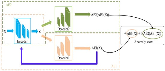
Figure 2.
USAD Model Detection Architecture Diagram.
2.2.2. LSTM-AE Model
A traditional autoencoder (AE) consists of an input layer, a hidden layer and an output layer. In the training phase, by reconstructing normal samples, the AE learns the data distribution characteristics of normal samples, and thus can reconstruct normal data effectively. In order to enhance the ability of traditional AE to process time-series data, a two-layer LSTM network is used in this paper to replace the fully-connected layer in traditional AE to form an LSTM-AE network, and this network structure is used as the three base models, AE1, AE2, and AE3, in the High-LowDAAE model proposed in this paper.
Recurrent neural networks (RNNs) suffer from the problems of gradient vanishing and gradient explosion, where gradient explosion can be solved by gradient truncation, i.e., manually trimming the gradient that exceeds a threshold to a certain range. However, tiny gradients due to the long-term dependency problem cannot be solved by similar methods, and artificially increasing the gradient value may impair the model’s ability to capture long-term dependency. LSTM effectively solves the long-term dependency problem by introducing a gating mechanism to control the transmission and loss of information flow. The structure of the LSTM-AE network is shown in Figure 3. The basic LSTM-AE model includes an encoder and a decoder, in which both the encoder and the decoder adopt a two-layer LSTM-connected structure, in which the first layer of the LSTM network extracts the timing features after compressing the input timing data, and then the extracted features are then fed into the second layer of the LSTM network to further extract the condensed timing features, the two-layer LSTM design is not only able to extract more The two-layer LSTM design can not only extract more effective timing features, but also output timing features with different compression levels. In Figure 3, Decoder1, Decoder2 and Decoder3 denote the three decoder layers used in AE1, AE2 and AE3, respectively, while Encoder is the coding layer shared by the three base models. Thus, LSTM-AE serves as the base model of High-LowDAAE to effectively capture the correlation in time-series data.
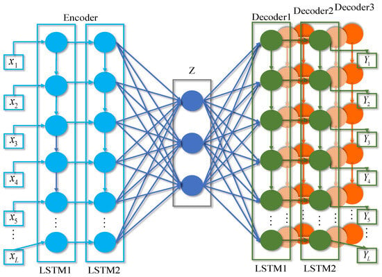
Figure 3.
LSTM-AE model diagrams.
2.2.3. High-LowDAAE Model
The High-LowDAAE model designed in this paper is shown in Figure 4. In the overall structure, firstly, the High-LowDAAE model adds an extra “discriminator” AE3 on the basis of the USAD model; secondly, the fully connected layers in the Encoder and decoder of the three basic AEs are replaced by a two-layer LSTM network, which is utilized as a basis for the LSTM-AE introduced in Section 3.1. self-encoder. In terms of function optimization, firstly, the High-LowDAAE model employs multi-scale temporal feature fusion. For the Encoder composed of the dual-layer LSTM network, the temporal features output through the single-layer LSTM network and the temporal features output through the dual-layer LSTM network are fed to Decoder1, respectively. The temporal features containing more information about the local and short-term patterns of the original sequence and those containing more long-term and global pattern information about the whole sequence are reconstructed, respectively, and the two parts of the output reconstructed data are weighted and fused to obtain the final reconstructed data. Secondly, AE2 and the newly added AE3 are reconstructed for and features, respectively, in order to enhance the reconstruction ability of Decoder2 and Decoder3 for different levels of temporal features (Decoder2 corresponding to the high-level temporal features, Decoder3 corresponds to low-level temporal features) and trained against AE1, respectively, to better enhance the reconstruction ability of AE1 on temporal data by combining high-level features and low-level features in the temporal data. The training process and detection process of the High-LowDAAE model are described in detail below.
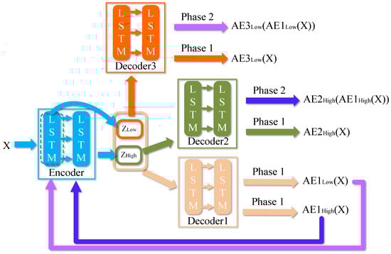
Figure 4.
High-LowDAAE Model Diagrams.
2.2.4. Training Phase
The High-LowDAAE model is similarly trained in two stages during the training phase. First, three AEs are trained to learn to reconstruct the normal input data X. Among them, AE1 reconstructs different levels of temporal features and , respectively, and weights and sums the reconstructed data and to obtain the final reconstructed data; whereas, AE2 reconstructs only the high-level feature individually, and AE3 reconstructs only the low-level feature , and the AE3’s Encoder has only a single-layer LSTM network. Second, AE2 and AE3 are trained against AE1, and unlike the USAD model, AE1 will utilize the reconstructed data of high-level features to “confuse” AE2, and the reconstructed data of low-level features to “confuse” AE3.
Phase 1: AE training. In the first stage, the goal is to train three AEs to reconstruct the input. The input data X is output by the encoder with high-level feature and low-level feature , respectively, and then reconstructed by the three decoders, respectively. Where for the reconstruction training of AE1, the reconstructed outputs obtained from the high level feature and low level feature by Decoder1 are weighted and summed, and make , as a way to merge different levels of temporal features to train the AE1, so that the goal of this phase of training is:
Phase 2: Dual adversarial training. In the second phase, the goal is to train AE2 and AE3 to distinguish the reconstructed data from AE1 and the real data, where AE3 distinguishes the reconstructed data with low-level features and AE2 distinguishes the reconstructed data with high-level features, and to train AE1 to “confuse” AE2 and AE3. The reconstructed data and from AE1 are again compressed into and by an encoder and then reconstructed by AE2 and AE3, respectively. The goal of AE1 in adversarial training is to minimize the difference between X and the outputs of AE2 and AE3. the goal of AE2 and AE3 is to maximize this difference. The training goal is:
The two training phase Losses are combined as follows:
where denotes a training period.
2.2.5. Detection Phase
After completing offline training, the High-LowDAAE model enters the detection phase. In the detection stage, the input data passes through the encoding layer and outputs the high-level hidden variable and the low-level hidden variable , respectively. and pass through Decoder1 to obtain AE1, which is the reconstructed fusion output for different temporal features. Then, re outputs the high-level and low-level features through the encoder. The high-level features pass through Decoder2 to obtain the reconstructed output for the high-level features, and the low-level features pass through Decoder3 to obtain the reconstructed output for the low-level features. Finally, the weighted sum of the reconstruction errors of the three reconstructed outputs relative to the input data is defined as the anomaly score:
In the detection phase, the High-LowDAAE model retains the and parameters of the USAD model for anomaly score computation, with the difference that the High-LowDAAE model takes full advantage of the timing characteristics of the different layers.
3. Performance Analysis of High-LowDAAE Model
3.1. Experimental Data and Parameter Setting
In this paper, we use the electricity consumption dataset released by the State Grid Corporation of China (SGCC) to detect abnormal electricity consumption in real scenarios, and construct three sub-datasets consisting of 1000, 5000, and 10,000 pieces of user data, respectively, each of which consists of 1036d of electricity consumption, and each day of electricity consumption of a user constitutes an attribute of that user. The statistical information of the datasets is shown in Table 2.
Table 2.
Dataset statistics.
Based on the setting of model and training parameters, in the basic LSTM-AE network, the first layer of LSTM hidden layer is 128, the second layer is 64, and the Relu activation function is used between each layer; During training, set a learning rate of 0.001 and use the Adam optimizer to train the model with an epoch of 100 and a batch size of 512. During training, three sub-datasets were trained and tested separately. Only the entire Nomaly dataset was used during training, with a ratio of 8:2 for the training and validation sets. The entire dataset was used for testing, and the size of the temporal window was set to 12.
In the setting of model parameters and training parameters, the first LSTM hidden layer is 128 and the second layer is 64 in the basic LSTM-AE network, and the Relu activation function is used between each layer; during training, a learning rate of 0.001 is set and the model is trained using the Adam optimizer, the epoch is set to 100, and the batch size is 512. In training time, the three sub-datasets are trained and tested separately, only the whole Nomaly data is used for training, and the whole dataset is used for testing, and the size of the timing window is set to 12.
In order to comprehensively evaluate the performance of the algorithm, the experiments are evaluated by the F1 value, which is a weighted average of the accuracy and recall of the model.
3.2. Analysis of Ablation Experiments
This article set up four sets of ablation experiments on three sub-datasets to verify the effectiveness of our improvement. The F1 values on the three test sets are shown in Table 3 and Figure 5. In the three sub-datasets, the highest F1 value of the benchmark model USAD reached 0.852, indicating that the USAD model has a certain ability to distinguish between normal and abnormal samples; The second set of experiments began to test the effectiveness of the improvements made in this paper. The AE in the USAD model was replaced by the LSTM-AE network designed in this paper, and the F1 values on all three datasets were improved by 0.911, 0.824, and 0.787, respectively. This indicates that the LSTM-AE structure can help the model better capture long-term dependencies in temporal data, thereby improving its ability to detect abnormal samples. In the third group of experiments, only adding a new “discriminator” AE3 without replacing LSTM-AE resulted in an improvement in F1 values on all three test sets. However, the increase in F1 values was smaller than adding only LSTM-AE networks, with values of 0.901, 0.814, and 0.775, respectively. This indicates that for anomaly detection of temporal data, capturing temporal features between data is more important. However, the addition of dual “discriminators” also improves the data reconstruction ability. In the fourth experiment, LSTM-AE and AE3 were added simultaneously to test the performance of the High-LowDAAE model. As shown in Table 3, the F1 value of the High-LowDAAE model on the three sub-datasets was once again improved compared to only adding LSTM-AE and AE3, reaching 0.927, 0.853, and 0.815 in the three sub-datasets, respectively. This indicates that after fusing temporal features at different levels of high and low, the model’s ability to reconstruct temporal data is once again improved, and it can better detect abnormal electricity consumption data.
Table 3.
Comparison results of ablation experiments.
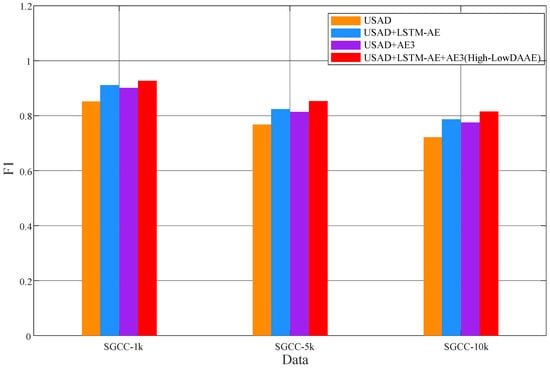
Figure 5.
Comparison results of ablation experiments.
3.3. Comparative Experimental Analysis
This article selects four of the latest anomaly detection models as benchmark models to compare the performance of the proposed High-LowDAAE model, namely IF, OmniAnomaly, LSTM-VAE, and MAD-GAN. The experiments of all models were conducted under the same conditions.
The testing results of this model on three sub-datasets, including IF, OmniAnomaly, LSTM-VAE, and MAD-GAN, are shown in Figure 6 and Table 4. The F1 values of the High-LowDAAE model are higher than those of other models on all three sub-datasets, with the IF algorithm performing the worst, far behind the other three deep-learning-based algorithms, with values of 0.821, 0.747, and 0.694 in the three sub-datasets, respectively. Among other deep-learning-based algorithms, OmniAnomaly and LSTM-VAE both enhance VAE’s feature extraction ability for temporal data by adding various efficient recurrent neural networks (such as GRU and LSTM) to the VAE model. They model the long-term dependencies of temporal data and perform well on all three sub-datasets. Among them, OmniAnomaly has F1 values of 0.894, 0.842, and 0.763 in the three sub-datasets, while LSTM-VAE has F1 values of 0.865, 0.811, and 0.736 in the three sub-datasets, respectively. The MAD-GAN model incorporates LSTM on the basis of the GAN network, allowing the model to conduct adversarial training on more temporal features. Its performance is second only to OmniAnomaly, reaching 0.871, 0.821, and 0.741, respectively. From this, it can be seen that adversarial training and rich temporal features are the key to improving the accuracy of the model when detecting anomalies in temporal data. Therefore, the High-LowDAAE model designed in this paper not only integrates temporal features from different levels, but also designs a more advanced adversarial training model. The dual “discriminators” form better integrates temporal features from different levels, ultimately improving the accuracy of the model in detecting abnormal electricity consumption behavior, leading the other four models.
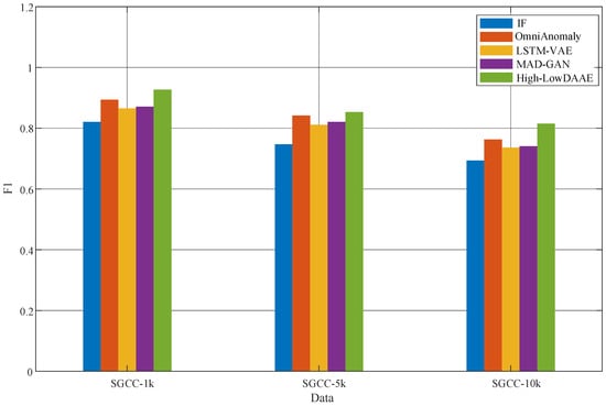
Figure 6.
Comparative experimental results.
Table 4.
Comparative experimental results.
As shown in Figure 7, the visualization of the High-LowDAAE model designed in this paper with IF, OmniAnomaly, LSTM-VAE and MAD-GAN for normal and abnormal data reconstruction is demonstrated. From the figure, it can be seen that the reconstruction ability of different models for normal data is relatively similar; however, for abnormal data, the IF algorithm represented by the blue line segment does not output reconstructed data with a very low similarity to the abnormal data, i.e., the reconstruction error is very small, and it is not capable of detecting the abnormal data very well, whereas the other three models based on the foundation of deep learning are constantly enlarging the reconstruction error when they are fed with abnormal data, and have a have some detection ability, but for the data that is extremely similar to normal data, OmniAnomaly, LSTM-VAE and MAD-GAN models, there is also no reconstruction error that exceeds the threshold, and thus there is a missed detection. The reconstruction of the High-LowDAAE model for the anomalous data makes it very close to the normal data, and thus the amplification of the reconstruction error for the General Assembly is obvious, as shown in the green line segment in Figure 7.
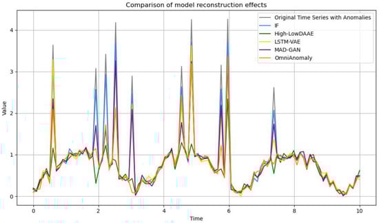
Figure 7.
Comparison of model reconstruction effects.
The reconstructed output of High-LowDAAE model for all the data is very close to the normal data, so even if the abnormal data is more hidden and very similar to the normal data, the High-LowDAAE model is still able to detect it well. From Table 5, it can be more intuitively seen that the High-LowDAAE model has a higher reconstruction error for abnormal data. Compared to the worst-performing IF, the reconstruction error is 4.65 times higher. The reconstruction errors of LSTM-VAE and MAD-GAN models are relatively similar, with values of 0.35 and 0.37, respectively. The reconstruction error of OmniAnomaly is second only to High-LowDAAE, with a value of 0.55.
Table 5.
Comparison of reconstruction errors of abnormal data points of different models.
4. Conclusions
In this paper, we focus on the problem of abnormal power usage behavior detection of power system users and design a model High-LowDAAE for abnormal power usage behavior detection. Considering that many models ignore the problem of temporal correlation in time series, we first replace the fully connected layer in the AE model with a two-layer LSTM network and use the designed LSTM-AE model as the base self-encoder model in this paper. By introducing LSTM, we can capture the long-range dependencies in the time-series data. Secondly, the USAD model is improved by replacing all the base AEs in USAD with LSTM-AEs and adding a new “discriminator” AE3 on top of them, and when AE2 and AE3 are trained in parallel against each other, the temporal features from different layers are used to train AE2 and AE3 separately in this paper. By using richer temporal features than a single level to improve the reconstruction ability of AE1 for different normal time-series data, we can maximize the reconstruction error when inputting abnormal data. Finally, the unsupervised learning method is used to detect unknown anomalies that may exist in the electricity consumption of grid users. For the proposed method, we first conduct ablation experiments to validate the effectiveness of each step of improvement of High-LowDAAE and highlight the importance of temporal correlation for anomaly detection of time-series data. Then, this paper conducts comparison experiments with four other algorithmic models to verify the effectiveness of this paper’s algorithm in anomalous electricity behavior detection.
Author Contributions
Conceptualization, C.T.; methodology, C.T.; software, C.T.; validation, C.T., Y.Q. and Y.L.; formal analysis, C.T. and Y.L.; investigation, C.T. and Y.Q.; resources, Y.Q. and Y.L.; data curation, H.P.; writing—original draft preparation, C.T.; writing—review and editing, C.T. and H.P.; visualization, C.T.; supervision, Z.T.; project administration, Z.T.; funding acquisition, Z.T. All authors have read and agreed to the published version of the manuscript.
Funding
The research was supported by NSFC (Grant No 62172146, U23A20317).
Data Availability Statement
The experimental data in this paper comes from the public dataset of State Grid Corporation of China (SGC).
Conflicts of Interest
The authors declare no conflicts of interest.
References
- Gungor, V.C.; Sahin, D.; Kocak, T.; Ergut, S.; Buccella, C.; Cecati, C.; Hancke, G.P. Smart Grid Technologies: Communication Technologies and Standards. IEEE Trans. Ind. Inform. 2011, 7, 529–539. [Google Scholar] [CrossRef]
- Song, Y.Q.; Zhou, G.L.; Zhu, Y.L. Present Status and Challenges of Big Data Processing in Smart Grid. Power Syst. Technol. 2013, 37, 927–935. [Google Scholar]
- Zhang, W.; Liu, Z.; Wang, M.; Yang, X. Research Status and Development Trend of Smart Grid. Power Syst. Technol. 2009, 33, 1–11. [Google Scholar]
- Bayindir, R.; Hossain, E.; Vadi, S. The path of the smart grid -the new and improved power grid. In Smart Grid Workshop and Certificate Program; IEEE: Piscataway, NJ, USA, 2016; pp. 1–8. [Google Scholar]
- Ge, Z.; Yu, Y.; Zheng, S.S.; Cai, C.Y.; Shan, H. The Impact of Electricity Theft on Power Supply Systems and Anti Electricity Theft Systems. Technol. Entrep. Mon. 2012, 12, 198–199. [Google Scholar]
- Esling, P.; Agon, C. Time-series data mining. ACM Comput. Surv. 2012, 45, 1–34. [Google Scholar] [CrossRef]
- Wang, B.; Mao, Z. A dynamic ensemble outlier detection model based on an adaptive k-nearest neighbor rule. Inf. Fusion 2020, 63, 30–40. [Google Scholar] [CrossRef]
- Panigrahi, S.; Kundu, A.; Sural, S.; Majumdar, A.K. Credit card fraud detection: A fusion approach using Dempster-Shafer theory and Bayesian learning. Inf. Fusion 2009, 10, 354–364. [Google Scholar] [CrossRef]
- Wang, B.; Mao, Z.Z. Outlier detection based on a dynamic ensemble model: Applied to process monitoring. Inf. Fusion 2019, 51, 244–258. [Google Scholar] [CrossRef]
- Angelos, E.W.S.; Saavedra, O.R.; Cortés, O.A.C.; De Souza, A.N. Detection and Identification of Abnormalities in Customer Consumptions in Power Distribution Systems. IEEE Trans. Power Deliv. 2011, 26, 2436–2442. [Google Scholar] [CrossRef]
- Sun, Y.; Li, S.H.; Cui, C.; Li, B.; Chen, S.; Cui, G. Improved Outlier Detection Method of Power Consumer Data Based on Gaussian Kernel Function. Power Syst. Technol. 2018, 42, 1595–1604. [Google Scholar]
- Zhuang, C.; Zhang, B.; Hu, J.; Li, Q.; Zeng, R. Anomaly Detection for Power Consumption Patterns Based on Unsupervised Learning. Proc. CSEE 2016, 36, 379–387. [Google Scholar]
- Xu, G.; Tan, Y.P.; Dai, T.H. Sparse Random Forest Based Abnormal Behavior Pattern Detection of Electric Power User Side. Power Syst. Technol. 2017, 41, 1964–1973. [Google Scholar]
- Jindal, A.; Dua, A.; Kaur, K.; Singh, M.; Kumar, N.; Mishra, S. Decision Tree and SVM-based Data Analytics for Theft Detection in Smart Grid. IEEE Trans. Ind. Inform. 2016, 12, 1005–1016. [Google Scholar] [CrossRef]
- Yan, Z.Z.; Wen, H. Electricity theft detection base on extreme gradient boosting in AMI. IEEE Trans. Instrum. Meas. 2021, 70, 1–9. [Google Scholar] [CrossRef]
- Zheng, K.D.; Kang, C.Q.; Hunagpu, F.Y. Detection Methods of Abnormal Electricity Consumption Behavior: Review and Prospect. Autom. Electr. Power Syst. 2018, 42, 189–199. [Google Scholar]
- Zheng, Z.; Yang, Y.; Niu, X.; Dai, H.N.; Zhou, Y. Wide & Deep Convolutional Neural Networks for Electricity-theft Detection to Secure Smart Grids. IEEE Trans. Ind. Inform. 2018, 14, 1606–1615. [Google Scholar]
- Dong, L.H.; Xiao, C.L.; Ye, O.; Yu, Z.H. A detection method for stealing electric theft based on CAEs-LSTM fusion model. Power Syst. Prot. Control. 2022, 50, 118–127. [Google Scholar]
- Lei, Y.; Karimi, H.R.; Cen, L.; Chen, X.; Xie, Y. Processes soft modeling based on stacked autoencoders and wavelet extreme learning machine for aluminum plant-wide application. Control Eng. Pract. 2021, 108, 104706. [Google Scholar] [CrossRef]
- Rao, L.; Pang, T.; Ji, R.; Chen, X.; Zhang, J. Combined with Stack Autoencoder-Extreme Learning Machine Method. Prog. Laser Optoelectron. 2019, 56, 247–253. [Google Scholar]
- Xu, M.J.; Zhao, J.; Wang, S.Y.; Xuan, Y.; Chen, B.J. A multi-task joint modeling-based approach for classifying residential electricity usage patterns. J. Electrotechnol. 2022, 37, 5490–5502. [Google Scholar]
- Chen, L.; Fang, Q.; Chen, Y. Intelligent Clothing Interaction Design and Evaluation System Based on DCGAN Image Generation Module and Kansei Engineering. J. Phys. Conf. Ser. 2021, 1790, 0102025. [Google Scholar] [CrossRef]
- Audibert, J.; Michiardi, P.; Guyard, F. USAD: Unsupervised anomaly detection on multivariate time series. In Proceedings of the 26th ACM SIGKDD Conference on Knowledge Discovery and Data Mining, Virtual Event, 23–27 August 2020; ACM: New York, NY, USA, 2020; pp. 3395–3404. [Google Scholar]
- Cai, J.H.; Wang, K.; Dong, K.; Yao, Y.H.; Zhang, Y.F. Power user stealing detection based on DenseNet and random forest. J. Comput. Appl. 2021, 41, 75–80. [Google Scholar]
Disclaimer/Publisher’s Note: The statements, opinions and data contained in all publications are solely those of the individual author(s) and contributor(s) and not of MDPI and/or the editor(s). MDPI and/or the editor(s) disclaim responsibility for any injury to people or property resulting from any ideas, methods, instructions or products referred to in the content. |
© 2024 by the authors. Licensee MDPI, Basel, Switzerland. This article is an open access article distributed under the terms and conditions of the Creative Commons Attribution (CC BY) license (https://creativecommons.org/licenses/by/4.0/).