Figure 1.
The arrangement of conductors in a three-phase single-layer machine with slots and poles. The rows of the table stand for, respectively, slot number, and the first layer. Each color and number are associated with a phase.
Figure 1.
The arrangement of conductors in a three-phase single-layer machine with slots and poles. The rows of the table stand for, respectively, slot number, and the first layer. Each color and number are associated with a phase.
Figure 2.
The phase diagram for a three-phase single-layer induction motor with slots and poles where each color represents a phase. The dashed lines are the individual phasor voltage from each slot while the solid line is the resultant phasor voltage. is the angle between the phases.
Figure 2.
The phase diagram for a three-phase single-layer induction motor with slots and poles where each color represents a phase. The dashed lines are the individual phasor voltage from each slot while the solid line is the resultant phasor voltage. is the angle between the phases.
Figure 3.
Illustration of “right member” shift of the primitive winding distribution tables of normal and non-reduced systems.
Figure 3.
Illustration of “right member” shift of the primitive winding distribution tables of normal and non-reduced systems.
Figure 4.
Illustration of the swap of quadrants 1 and 3 of primitive winding distribution tables of reduced systems.
Figure 4.
Illustration of the swap of quadrants 1 and 3 of primitive winding distribution tables of reduced systems.
Figure 5.
The arrangement of conductors in a machine with phases, slots, poles, double layer, and coil pitch of slots. The rows of the table stand for, respectively, the slot number, the first layer, and the second layer. Each color and number are associated with a phase.
Figure 5.
The arrangement of conductors in a machine with phases, slots, poles, double layer, and coil pitch of slots. The rows of the table stand for, respectively, the slot number, the first layer, and the second layer. Each color and number are associated with a phase.
Figure 6.
The MMF curve of a machine with phases, slots, double layer, and coil pitch of .
Figure 6.
The MMF curve of a machine with phases, slots, double layer, and coil pitch of .
Figure 7.
Composition of the MMF of phase 1 of a three-phase single-layer machine with slots and poles. (a) MMF produced by conductors of phase 1 belonging to slot 1. (b) MMF produced by a 1-phase coil placed in slots 1 and 7.
Figure 7.
Composition of the MMF of phase 1 of a three-phase single-layer machine with slots and poles. (a) MMF produced by conductors of phase 1 belonging to slot 1. (b) MMF produced by a 1-phase coil placed in slots 1 and 7.
Figure 8.
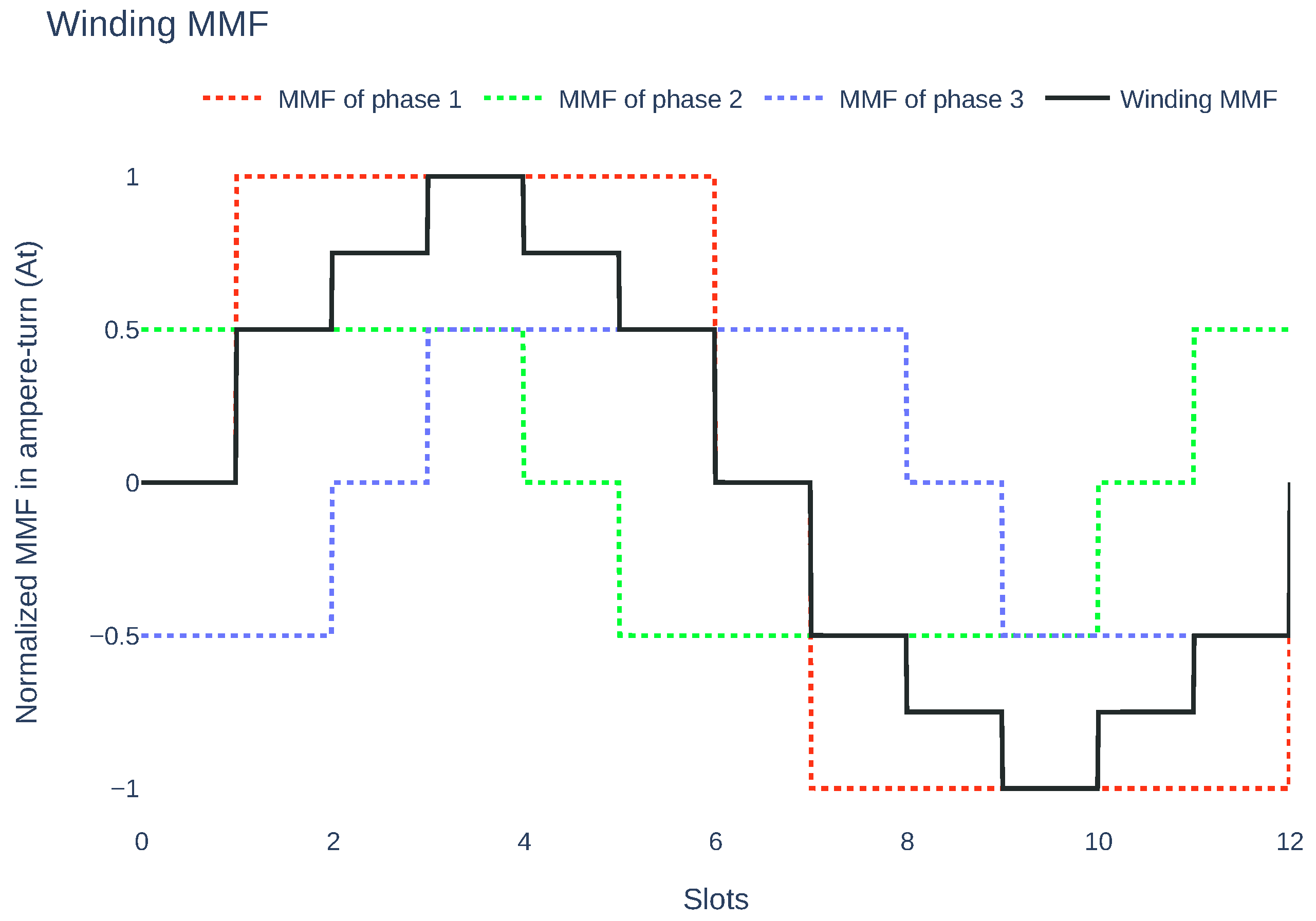
Total MMF curve composition of a three-phase single-layer machine with slots and poles.
Figure 8.
Total MMF curve composition of a three-phase single-layer machine with slots and poles.
Figure 9.
Fourier series approximation of the MMF curve of a three-phase single-layer machine with slots and poles.
Figure 9.
Fourier series approximation of the MMF curve of a three-phase single-layer machine with slots and poles.
Figure 10.
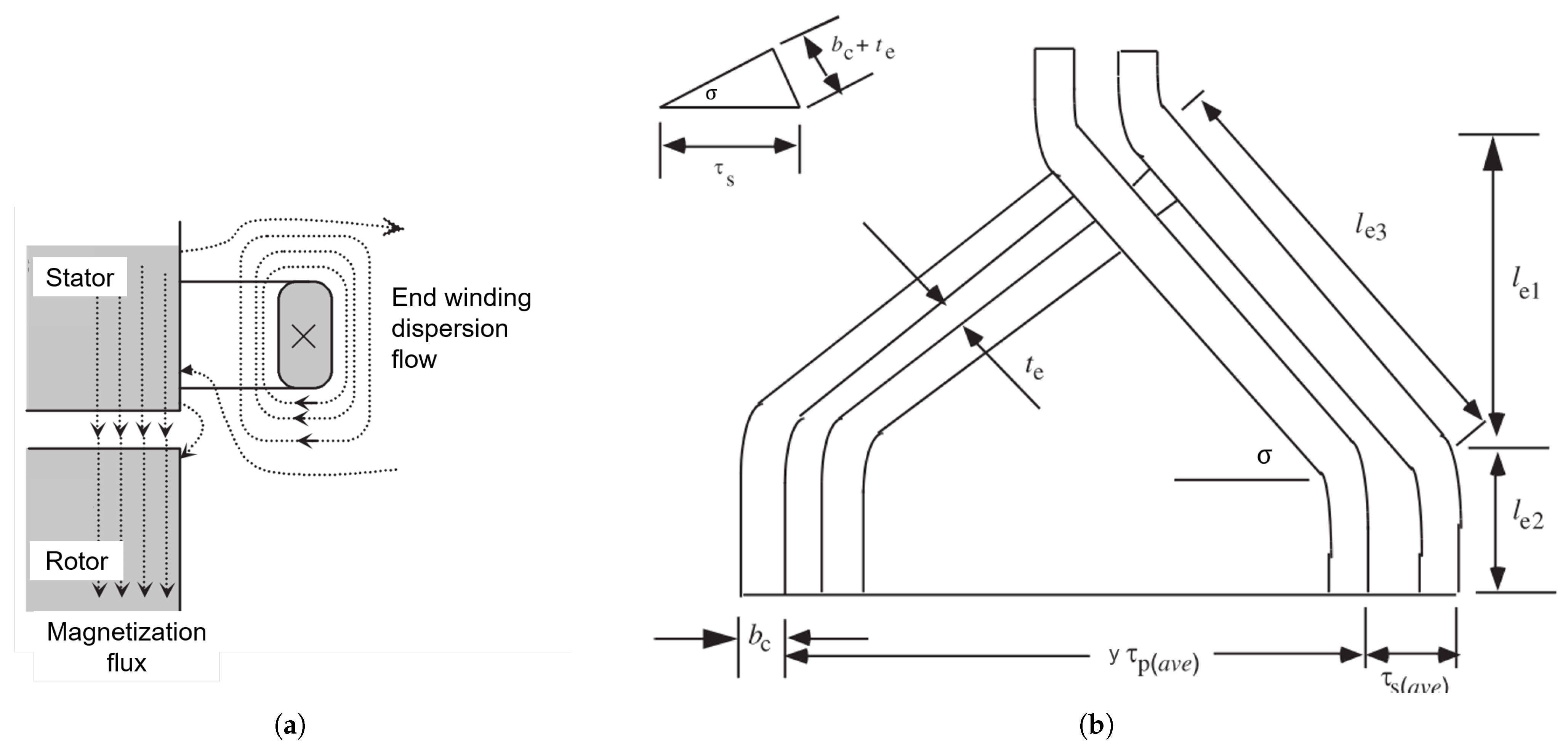
Illustration of end-winding dispersion flux. (a) The end-winding dispersion flux in side cutaway view. (b) Two adjacent diamond coil ends of an electrical machine stator.
Figure 10.
Illustration of end-winding dispersion flux. (a) The end-winding dispersion flux in side cutaway view. (b) Two adjacent diamond coil ends of an electrical machine stator.
Figure 11.
The evolution of the Pareto frontier during a bi-objective optimization problem solving. The green points stand for non-dominated solutions, the blue points are the dominated solutions, and the yellow point is the solution for which the density is being calculated. The hatched area is the area delimited by constraints. (a) The beginning of optimization. The Pareto frontier is far from the optimized solution set. (b) The expected optimization results. The Pareto frontier is at the limit of the restrictions to achieve the set of optimized solutions. (c) The density criterion computation for the yellow solution.
Figure 12.
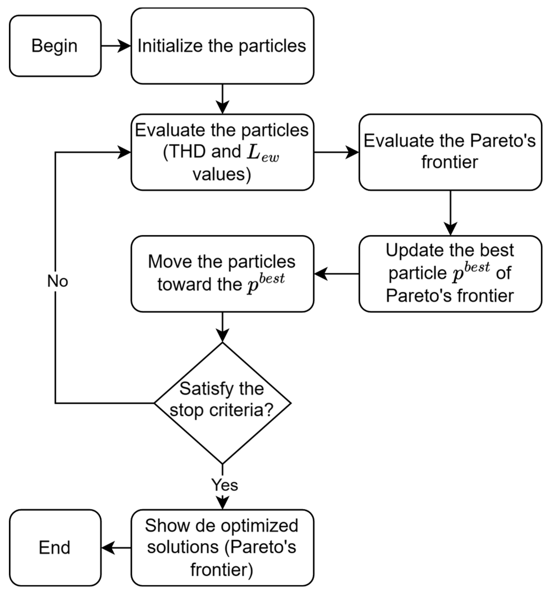
Flow diagram of the methodology applied to optimize the windings.
Figure 12.
Flow diagram of the methodology applied to optimize the windings.
Figure 13.
Ideal Pareto frontier and MOPSO for validation scenario 1.
Figure 13.
Ideal Pareto frontier and MOPSO for validation scenario 1.
Figure 14.
Ideal Pareto frontier and MOPSO for validation scenario 2.
Figure 14.
Ideal Pareto frontier and MOPSO for validation scenario 2.
Figure 15.
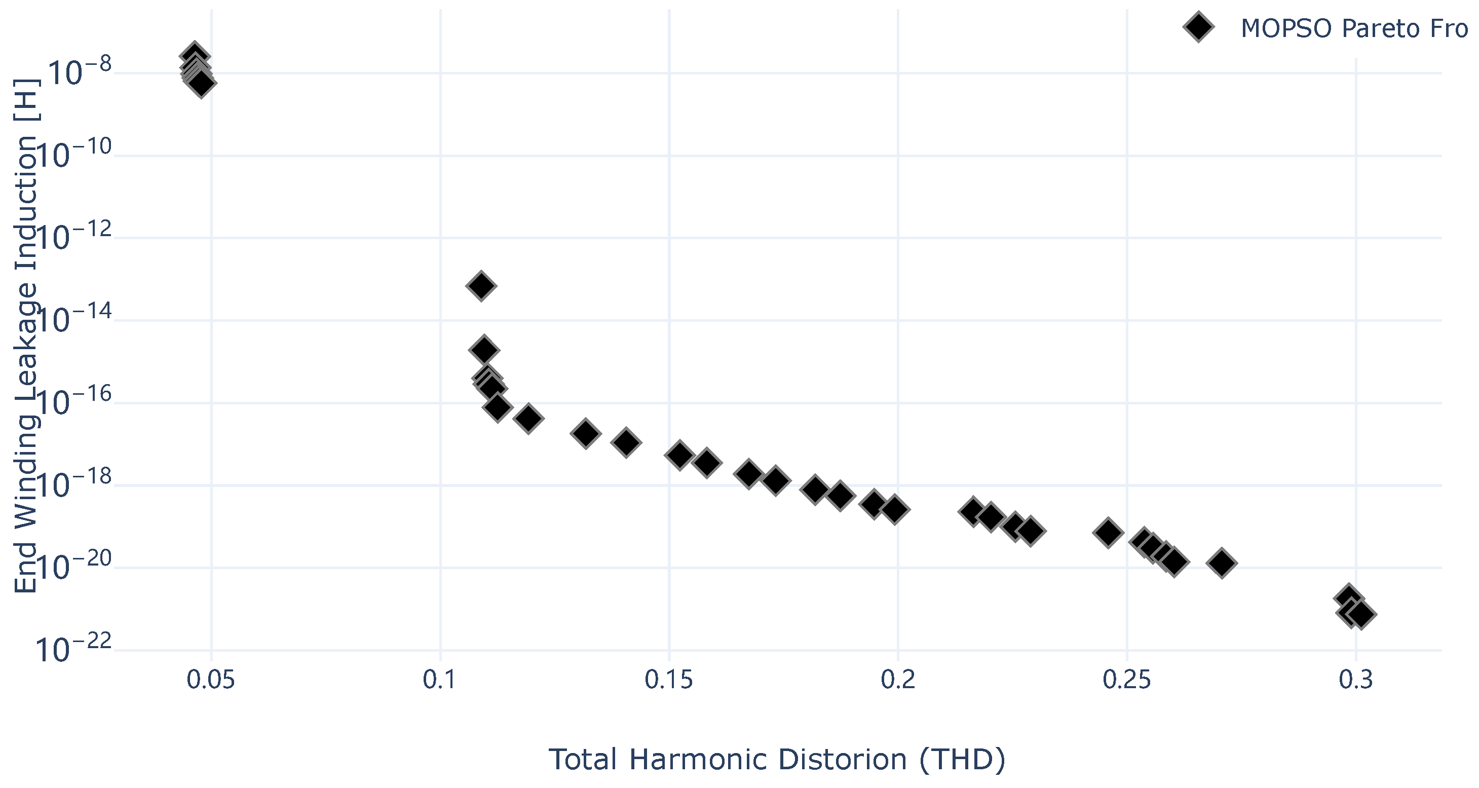
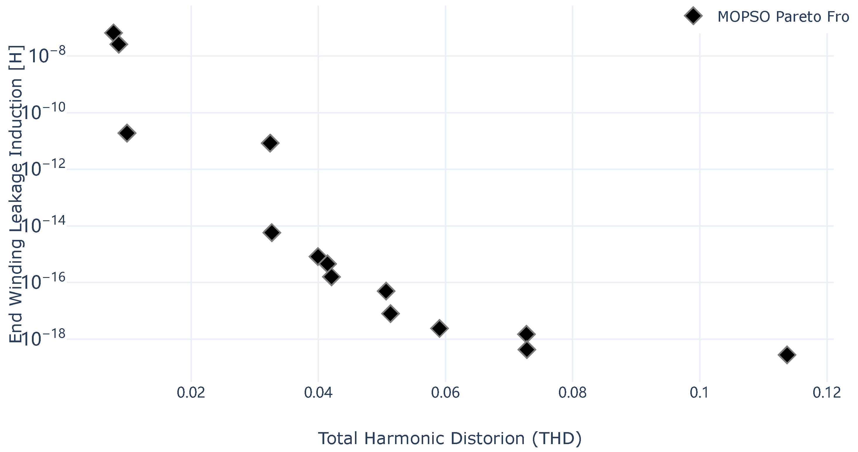
Pareto frontier computed by MOPSO for application scenario 1.
Figure 15.
Pareto frontier computed by MOPSO for application scenario 1.
Figure 16.
Pareto frontier computed by MOPSO for application scenario 2.
Figure 16.
Pareto frontier computed by MOPSO for application scenario 2.
Figure 17.
Pareto frontier computed by MOPSO for application scenario 3.
Figure 17.
Pareto frontier computed by MOPSO for application scenario 3.
Table 1.
EMF associated with the first phase in a three-phase single-layer induction motor with slots and poles.
Table 1.
EMF associated with the first phase in a three-phase single-layer induction motor with slots and poles.
| Slots | Current Direction | (deg) | Phasor |
|---|
| 1 | | 0 | |
| 2 | | 30 | |
| 7 | | 180 | |
| 8 | | 210 | |
| 13 | | 360 | |
| 14 | | 390 | |
| 19 | | 540 | |
| 20 | | 570 | |
| − | − | − | |
Table 2.
EMF associated with the winding of a three-phase single-layer induction motor with slots and poles.
Table 2.
EMF associated with the winding of a three-phase single-layer induction motor with slots and poles.
| Phasor |
|---|
| |
| |
| |
Table 3.
Basic structure of the winding distribution table.
Table 3.
Basic structure of the winding distribution table.
| | … | |
| | … | |
| ⋮ | ⋮ | ⋱ | ⋮ |
| | … | |
Table 4.
Primitive winding distribution table of a three-phase single-layer machine with slots and poles.
Table 4.
Primitive winding distribution table of a three-phase single-layer machine with slots and poles.
| 1 | 13 | 2 | 14 | 3 | 15 | 4 | 16 |
| 5 | 17 | 6 | 18 | 7 | 19 | 8 | 20 |
| 9 | 21 | 10 | 22 | 11 | 23 | 12 | 24 |
Table 5.
Sub-table 1 of winding distribution of a three-phase single-layer machine with slots and poles.
Table 5.
Sub-table 1 of winding distribution of a three-phase single-layer machine with slots and poles.
Table 6.
Sub-table 2 of winding distribution of a three-phase single-layer machine with slots and poles.
Table 6.
Sub-table 2 of winding distribution of a three-phase single-layer machine with slots and poles.
Table 7.
Winding distribution table for a three-phase single-layer machine with slots and poles. Each color is associated with a phase.
Table 7.
Winding distribution table for a three-phase single-layer machine with slots and poles. Each color is associated with a phase.
| 1 | 13 | 2 | 14 | | | | |
| 5 | 17 | 6 | 18 | | | | |
| 9 | 21 | 10 | 22 | | | | |
Table 8.
Winding distribution table not yet reordered for reduced systems.
Table 8.
Winding distribution table not yet reordered for reduced systems.
| Phases | Col. 1 | ⋯ | Col. |
|---|
| 1 | ⋯ | ⋯ | ⋯ |
| ⋮ | ⋯ | ⋯ | ⋯ |
| ⋯ | ⋯ | ⋯ |
| ⋯ | ⋯ | ⋯ |
| ⋮ | ⋯ | ⋯ | ⋯ |
| m | ⋯ | ⋯ | ⋯ |
Table 9.
Reordered winding distribution table for reduced systems.
Table 9.
Reordered winding distribution table for reduced systems.
| Phases | Col. 1 | ⋯ | Col. |
|---|
| 1 | ⋯ | ⋯ | ⋯ |
| ⋯ | ⋯ | ⋯ |
| 2 | ⋯ | ⋯ | ⋯ |
| ⋯ | ⋯ | ⋯ |
| ⋮ | ⋯ | ⋯ | ⋯ |
| ⋯ | ⋯ | ⋯ |
| m | ⋯ | ⋯ | ⋯ |
Table 10.
Primitive WDT for a machine with phases, slots, double layer, and coil pitch of slots.
Table 10.
Primitive WDT for a machine with phases, slots, double layer, and coil pitch of slots.
| 1 | 17 | 2 | 18 | 3 | 19 | 4 | 20 |
| 5 | 21 | 6 | 22 | 7 | 23 | 8 | 24 |
| 9 | 25 | 10 | 26 | 11 | 27 | 12 | 28 |
| 13 | 29 | 14 | 30 | 15 | 31 | 16 | 32 |
Table 11.
First-layer WDT after swapping quadrants 1 and 4 and multiplying the “right member” by for a machine with phases, slots, double layer, and coil pitch of slots.
Table 11.
First-layer WDT after swapping quadrants 1 and 4 and multiplying the “right member” by for a machine with phases, slots, double layer, and coil pitch of slots.
| 1 | 17 | 2 | 18 | | | | |
| 5 | 21 | 6 | 22 | | | | |
| 3 | 19 | 4 | 20 | | | | |
| 7 | 23 | 8 | 24 | | | | |
Table 12.
The first-layer WDT after row reordering for a machine with phases, slots, double layer, and coil pitch of slots.
Table 12.
The first-layer WDT after row reordering for a machine with phases, slots, double layer, and coil pitch of slots.
| 1 | 17 | 2 | 18 | | | | |
| 3 | 19 | 4 | 20 | | | | |
| 5 | 21 | 6 | 22 | | | | |
| 7 | 23 | 8 | 24 | | | | |
Table 13.
The second-layer WDT for a machine with phases, slots, double layer, and coil pitch of slots.
Table 13.
The second-layer WDT for a machine with phases, slots, double layer, and coil pitch of slots.
| | | | 12 | 28 | 13 | 29 |
| | | | 14 | 30 | 15 | 31 |
| | | | 16 | 32 | 17 | 1 |
| | | | 18 | 2 | 19 | 3 |
Table 14.
Validating solution scenarios by the application.
Table 14.
Validating solution scenarios by the application.
| Scenario | m | Z | p | | y | Possibilities |
|---|
| 1 | 3 | 3–90 | 1–3 | 2 | 1–4 | 1056 |
| 2 | 6 | 120–180 | 3–5 | 1–2 | 1–6 | 1281 |
Table 15.
Application scenarios.
Table 15.
Application scenarios.
| Scenario | m | Z | p | | y | Possibilities |
|---|
| 1 | 3 | 3–300 | 1–6 | 1–2 | 1–4 | 8940 |
| 2 | 5–7 | 70–210 | 1–6 | 1–2 | 1–4 | 12,690 |
| 3 | 9–12 | 90–250 | 1–5 | 1–2 | 1–8 | 28,980 |


