1. Introduction
In the transient stability assessment (TSA) [
1] of power systems, the evaluation of rotor angle stability under large disturbances has always been one of the hot research topics. Among the three modes of rotor angle stability, one is oscillatory instability. It is characterized by appearing stable initially and later showing oscillatory instability. In data-driven transient stability binary assessments, oscillatory instability is easily misjudged as stable. This misjudgment poses a significant threat to the safe and stable operation of power systems [
2]. Therefore, it is urgent to construct a more accurate and rapid transient stability multi-class assessment model to ensure the reliable operation of the power grid.
Transient stability depends on the existence of both components of electromagnetic torque for each synchronous machine in the system [
3]. A lack of sufficient synchronizing torque results in aperiodic instability. Its judgment basis is the loss of synchronism during the first or second swing. In such a transient situation, targeted emergency control actions, such as generator tripping, reducing mechanical power of accelerating generators, forced excitation, etc., should be taken quickly to maintain stability and reduce loss resulting from system fault. In contrast to the aforementioned aperiodic instability due to a lack of synchronizing torque, insufficient damping torque results in oscillatory instability with increasing amplitude. Generators remain in synchronism during the first two swings, but the oscillation with increasing amplitude eventually destabilizes the power system. The judgment basis of oscillatory instability is that the rotor angle dynamics are undamped. For this oscillatory instability status, emergency controls, such as adding a wide-area damping controller to flexible AC transmission system (FACTS) devices [
4] or VSC-HVDC [
5], should be taken to suppress oscillation. Therefore, under different initial operating conditions as well as the nature of the disturbance, power systems exhibit different instability modes. The dominant factors of the two instability modes are different, so it is desirable that control actions be different in order to be effective.
There are two approaches to constructing multi-class assessment models based on data-driven methods. One is the direct method [
6], which only uses a single assessment model to identify the different modes of the power system. Shi et al. proposed a transient stability multi-class model based on a convolutional neural network (CNN). And this model was simulated and verified on the IEEE 39-bus power system, achieving an accuracy rate of 97.7% for the evaluation of three modes [
7]. Li et al. constructed an artificial feature set using bus voltage trajectory clusters and employed XGBoost for feature extraction and encoding. They used random forest for a multi-class assessment model, achieving high assessment accuracy and robustness [
8]. Shi et al. introduced a squeeze-and-excitation module into traditional convolutional neural networks [
9]. This module amplified useful feature channels while suppressing less effective ones. Therefore, the assessment model could more efficiently identify the stable state and leading instability modes of the power system, completing the recognition of stability, rotor angle instability, or voltage instability modes. Shi et al. proposed active deep learning based on a DIM intelligent recognition framework, which significantly reduced the number of labeled samples required [
10]. By using this approach, the assessment model could easily distinguish three states of the power system: stability, rotor angle instability, and voltage instability.
Another approach is the decomposition method [
11], which breaks down the multi-class problem into a decision fusion problem involving several binary classifiers. Kang et al. proposed a ‘One vs. One’ decomposition method, which searched the most suitable classification algorithm for each category and combined these classification algorithms to improve the classification accuracy of the model [
12]. A multi-label classification model was proposed by Xu et al. [
13], which decomposed the data into a ‘One vs. Rest’ approach. And the model was combined with an improved support vector machine to reduce computational costs. Chambers et al. applied models that perform excellently in the recognition tests of CNN and long short-term memory (LSTM) to a ‘Many to Many’ classification model [
14]. This significantly improved the model’s computational efficiency and classification accuracy. Bi et al. assigned different weights to different binary classifiers and combined this with the diversified one against one (DOVO) concept to improve classification accuracy under class imbalance [
15].
In practical applications, multi-class models constructed by the direct method usually have weaker generalization capabilities. And the classification accuracy of models will decrease under conditions of sample imbalance. This paper attempts to apply a multi-class assessment model based on CNN-LSTM-VAE-GAN (CLV-GAN) and improved error-correcting output code (I-ECOC) to further improve the accuracy of multi-class transient stability assessment models in power systems. The main research focuses on two issues: First, the study addresses the problem of reduced accuracy in binary classifiers resulting from sample imbalance. In the actual operation of power systems, the number of aperiodic unstable and oscillatory unstable samples is far less than that of stable samples. Conventional classifiers tend to classify difficult-to-classify minority unstable samples as belonging to the majority stable sample category, resulting in lower discrimination accuracy for unstable samples. However, because the number of unstable samples is far less than that of stable samples in the power system, the overall accuracy of the multi-class TSA model is not low. However, misjudging unstable samples as stable ones can lead to significant losses for the safe operation of power systems. Therefore, the paper proposes a data augmentation algorithm based on spatiotemporal features to reduce the loss caused by sample imbalance. The CLV-GAN algorithm first processes the bus voltage data into forms suitable for extracting temporal and spatial features. Then, the CLV-GAN algorithm employs LSTM and CNN as two feature extraction channels of the variational autoencoder (VAE) to learn the latent spatiotemporal distribution features of the data samples. New artificial samples will be generated by CLV-GAN based on the learned features. Finally, the artificial samples will be sent to the discriminator of the generative adversarial network (GAN) to further improve their quality. The model will also optimize the network parameters based on the results of the discrimination. Secondly, the study aims to further enhance the fault tolerance of the ECOC binary classifier. The fault tolerance of ECOC is not only related to the number of binary classifiers in the ECOC but also to the discrimination accuracy of each binary classifier when facing difficult-to-classify samples. Based on this, the paper proposes an improved error-correcting output code (I-ECOC) algorithm, which changes the output of binary classifiers in the ECOC to prediction probabilities and forms the prediction code with the prediction probabilities of each binary classifier. The I-ECOC algorithm significantly reduces the impact of difficult-to-classify samples on the model, improving the accuracy of the multi-class TSA model. Simulation analysis was conducted on the IEEE 39-bus and IEEE 140-bus power systems.
The main contributions of this paper are summarized below:
- (1)
Considering the spatiotemporal characteristics of power system samples, we propose an improved VAE-GAN network. The proposed network uses LSTM and CNN as the temporal and spatial encoders of VAE, respectively. Furthermore, we improve the discriminator of VAE-GAN by combining CNN and LSTM to enhance the quality of generated samples.
- (2)
We propose an improved error-correcting output code (I-ECOC) algorithm based on ECOC. The proposed I-ECOC algorithm changes the output of binary classifiers in the ECOC from +1/−1 to prediction probabilities and forms the new prediction code with the prediction probabilities of each binary classifier. Meanwhile, we also changed the composition of the ECOC encoding matrix for the new prediction codes.
This article has the following organization:
Section 1 introduces the significance of the research, the existing research methods and their limitations, as well as the research content of this article.
Section 2 introduces the principles of related technologies and the innovations of our work.
Section 3 carries out simulation analysis and discusses the simulation results. The conclusions and future research directions are discussed in
Section 4.
2. Methods
2.1. VAE
VAE is a generative model based on variational Bayesian inference [
16,
17]. It infers the probability distribution of latent variables of the original data through the encoder. Then, it samples latent variables from the distribution and decodes these latent variables through the decoder to generate samples. Assuming the original dataset is
and its latent variables are
, the posterior probability distribution of
can be obtained by the Bayesian formula, as shown in Equation (1):
where
represents the probability distribution of the variable
given the dataset
, from which sampling from
can obtain the latent variable
.
Since the distribution of the latent variable is difficult to observe directly, VAE introduces a simple distribution to approximate the indeterminate posterior distribution , assuming the posterior distribution follows a standard normal distribution and follows an ordinary normal distribution .
The Kullback–Leibler divergence (KLD), also known as the relative entropy, is widely used to measure the similarity between two distributions [
18]. Assuming a continuous interval
,
and
are two distinct probability density functions. The KLD for discrete random variables is shown in Equation (2):
The KLD for continuous random variables is shown in Equation (3):
where
and
.
The similarity between the two distributions
and
is measured by the KLD, and the calculation formula is shown in Equation (4):
where
and
represent the mean and variance of
, respectively;
and
represent the mean and variance of the
i-th sample, respectively; and
is the number of samples in the dataset.
Because the sampling process of
cannot be optimized using gradient descent, the reparameterization technique is adopted instead. Randomly sampling noise
from
and combining it with
and
to obtain
makes the sampling calculation from
transform into a numerical calculation that can be optimized by a gradient. The calculation formula is shown in Equation (5) and the network structure of VAE is illustrated in
Figure 1:
where
represents the
-th latent variable.
The decoder decodes the latent variable
to generate sample
, and the loss function of VAE is calculated as shown in Equation (6):
where
represents the training loss value of VAE, the first term on the right side of the equation is the KLD value between the posterior distribution learned by the VAE and the standard normal distribution, and the second term on the right side of the equation is the reconstruction error between the generated data and the original data.
2.2. GAN
The generative adversarial network (GAN) was proposed by Goodfellow et al. in 2014 [
19]. GAN can learn the probability density function of the distribution of the original dataset and generate a sample from the distribution of the real sample dataset. The GAN network mainly consists of two parts: the generator
G and the discriminator
D. The flowchart of GAN is shown in
Figure 2.
During the training process, the generator creates samples based on the input noise, while the discriminator distinguishes between the generated samples and the real samples. The training objective of the generator is to generate valid samples that closely match the real distribution as much as possible, while the training objective of the discriminator is to accurately identify the authenticity of the input samples. The two components engage in a continuous adversarial process during training, constantly improving. The loss functions for the generator and the discriminator are shown in Equations (7) and (8):
where
and
represent the
i-th generated sample and real sample, respectively;
is the loss of the discriminator;
is the loss of the generator;
represents the discriminator; and
is the number of samples.
During the alternating training process of the discriminator and the generator, the objective function of GAN is shown in Equation (9):
where
represents the mathematical expectation under a certain distribution, and
represents maximizing
while minimizing
.
2.3. ECOC
The decomposition method is a common approach to solving multi-class tasks, breaking down the multi-class learning task into multiple binary classification tasks for processing. Classic splitting strategies include One vs. One (OvO), One vs. Rest (OvR), and Many vs. Many (MvM) methods. The MvM strategy involves treating several classes as the positive class and several other classes as the negative class each time, thereby training several binary classifiers to achieve the purpose of solving multi-class tasks. Therefore, it can be seen that OvO and OvR are special cases of MvM [
20].
ECOC is a technique within the MvM strategy that combines encoding ideas with category splitting, aiming to improve the fault tolerance of decoding. ECOC mainly consists of two processes: encoding and decoding [
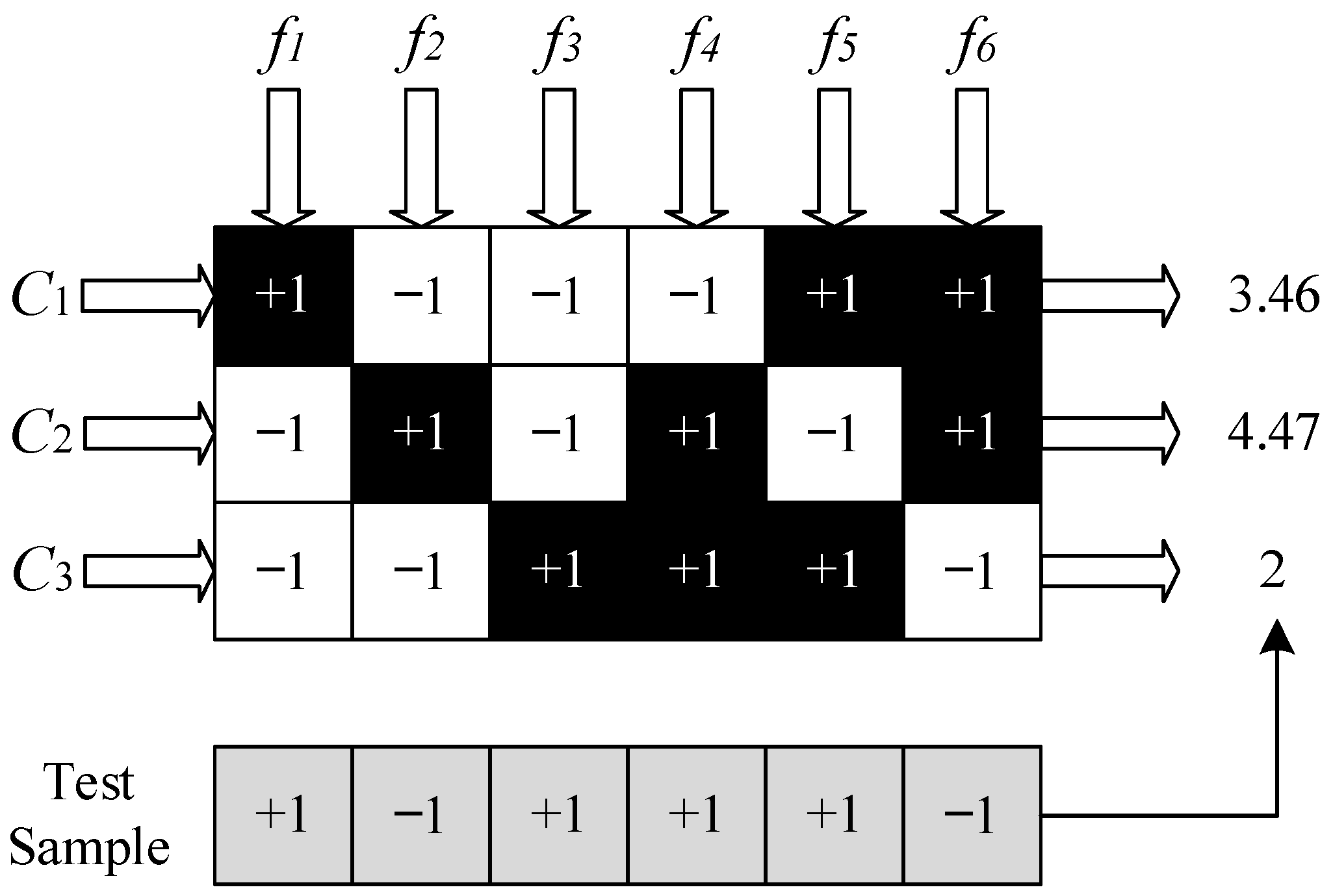
21]. In the encoding process, N categories are divided M times. Each division classifies a subset of category samples as positive and the remaining category samples as negative, thereby forming M binary training sets, and using these to train M binary classifiers. In the decoding process, M binary classifiers simultaneously predict the test sample and output the prediction results. Then, a prediction code is formed with M prediction results. Finally, by comparing the prediction code with the correct codes of N categories, the category with the smallest distance is returned as the final assessment result of ECOC.
Taking the classification of samples with categories
,
, and
as an example, six binary classifiers,
,
,
,
,
, and
, are constructed by the decomposition method. ECOC technology is applied for error-correcting coding discrimination, with the principle illustrated in
Figure 3. For each binary classifier, if its input belongs to the positive class, then the output is +1; otherwise, the output is −1. For example:
is trained and constructed by treating category
as the positive class and categories
and
as the negative classes. When the actual input sample belongs to category
, its output should be +1.
Figure 3 presents the encoding matrix corresponding to the correct identification of categories
,
, and
by binary classifiers
to
. In the decoding phase, the prediction code sequence of the actual input sample is composed of the prediction code values from each binary classifier. And the prediction code sequence is compared with the correct coding sequences corresponding to each category, and the category corresponding to the coding sequence with the smallest distance is output as the assessment result. Euclidean distance is used as the classification assessment criterion, as shown in Equation (10):
where
represents the correct output of the
i-th binary classifier
for the input sample,
represents the predicted output of
, and
is the number of binary classifiers.
For the test sample in
Figure 3, after ECOC prediction encoding, the Euclidean distance is calculated with the coding sequences of each category in the encoding matrix, indicating that the category of the test sample is
.
2.4. Multi-Class TSA Based on I-ECOC Encoding
2.4.1. Data Augmentation Algorithm CLV-GAN
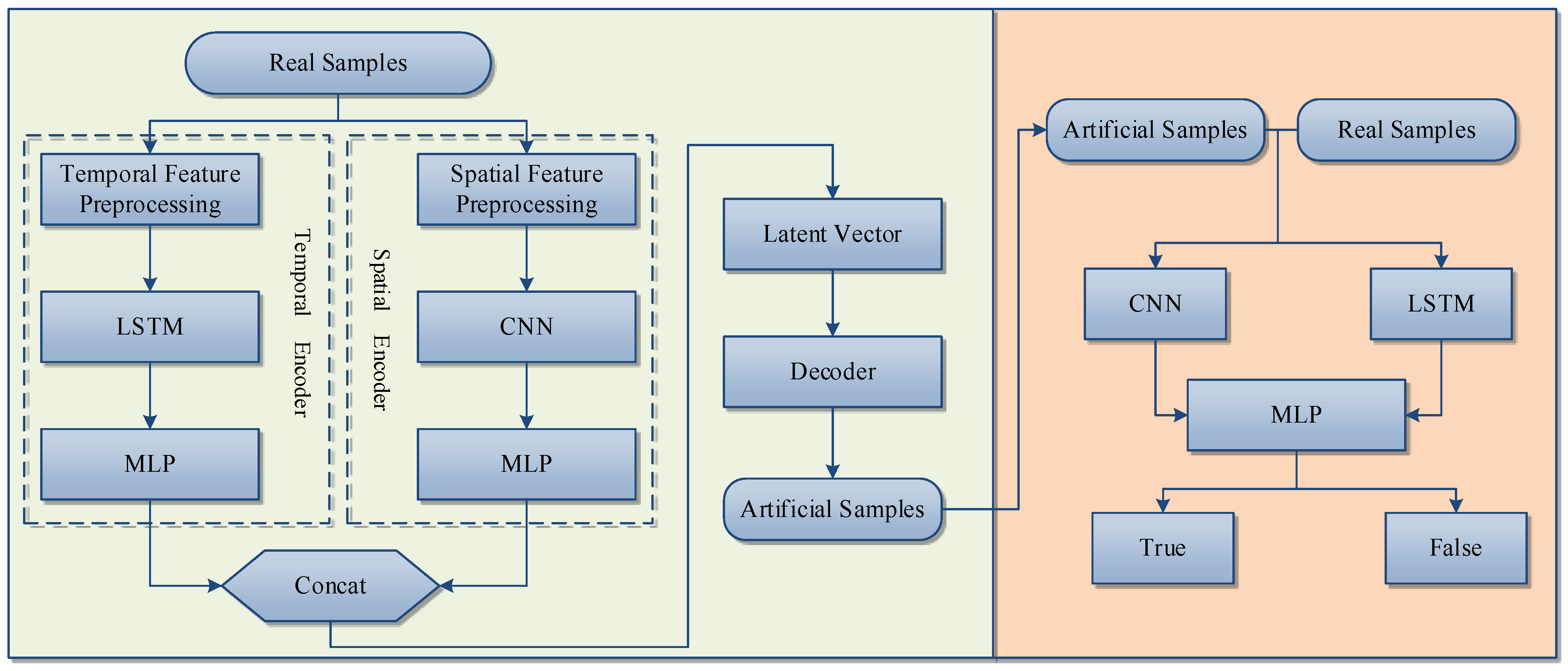
The loss function of VAE consists of two components: the KLD and the reconstruction loss. The KLD measures the difference between the distribution of generated samples and the distribution of real samples, while the reconstruction loss measures the dissimilarity between generated samples and real samples. During the neural network training process, although the reconstruction loss will approach zero as much as possible, this does not mean that the generated samples will become more realistic. To improve the quality of samples generated by VAE, the paper proposes a CLV-GAN model based on spatiotemporal dual encoding. A discriminator is added to judge the samples generated by VAE in order to enhance the realism of the generated samples in the VAE model. Simultaneously, the VAE network employs dual encoders for both temporal and spatial encoding. The temporal encoder fully learns the temporal characteristics of electrical data, while the spatial encoder learns the spatial characteristics of electrical data. Then, the outputs of these two encoders are concatenated and sent to the decoder for decoding to obtain artificial samples. Finally, the reconstruction loss of the generated samples is calculated and sent to the discriminator for judgment. To better discriminate the samples, the discriminator uses LSTM and CNN to extract features from the samples in terms of time and space, respectively. And the discrimination results is obtained through a multilayer perceptron (MLP). The algorithm flowchart of CLV-GAN is shown in
Figure 4.
In the algorithm process, the extraction of spatial features is achieved by reconstructing samples using the Hankel matrix [
22]. Assume the sample at the moment is:
where
represents the voltage value of the
-th bus at the
-th moment in data sample
.
The transformed matrix form is:
where
represents the Hankel matrix transformed from the sample at the
-th moment, and
represents the number of features in each row of the matrix.
The Hankel matrix retains all of the details of the original data while also extending it to a higher dimension. It converts power data samples from one-dimensional vectors into high-dimensional feature matrices, facilitating the extraction of their spatial global information. In the algorithm process, the preprocessing of temporal features involves converting samples into the form of time series, and the transformed matrix is shown in Equation (13):
where
represents the sample converted into the form of a time series, and
represents the voltage value of the
-th bus at the
-th moment.
The loss function of CLV-GAN mainly includes three parts: the KLD value between the latent variable distribution learned by the VAE encoder and the normal distribution, the reconstruction loss between the real samples and the samples generated by VAE, and the loss function of the discriminator. The calculation formula is shown in Equation (14):
where
represents the KLD value,
represents the reconstruction loss, and
represents the loss function of the discriminator.
2.4.2. I-ECOC
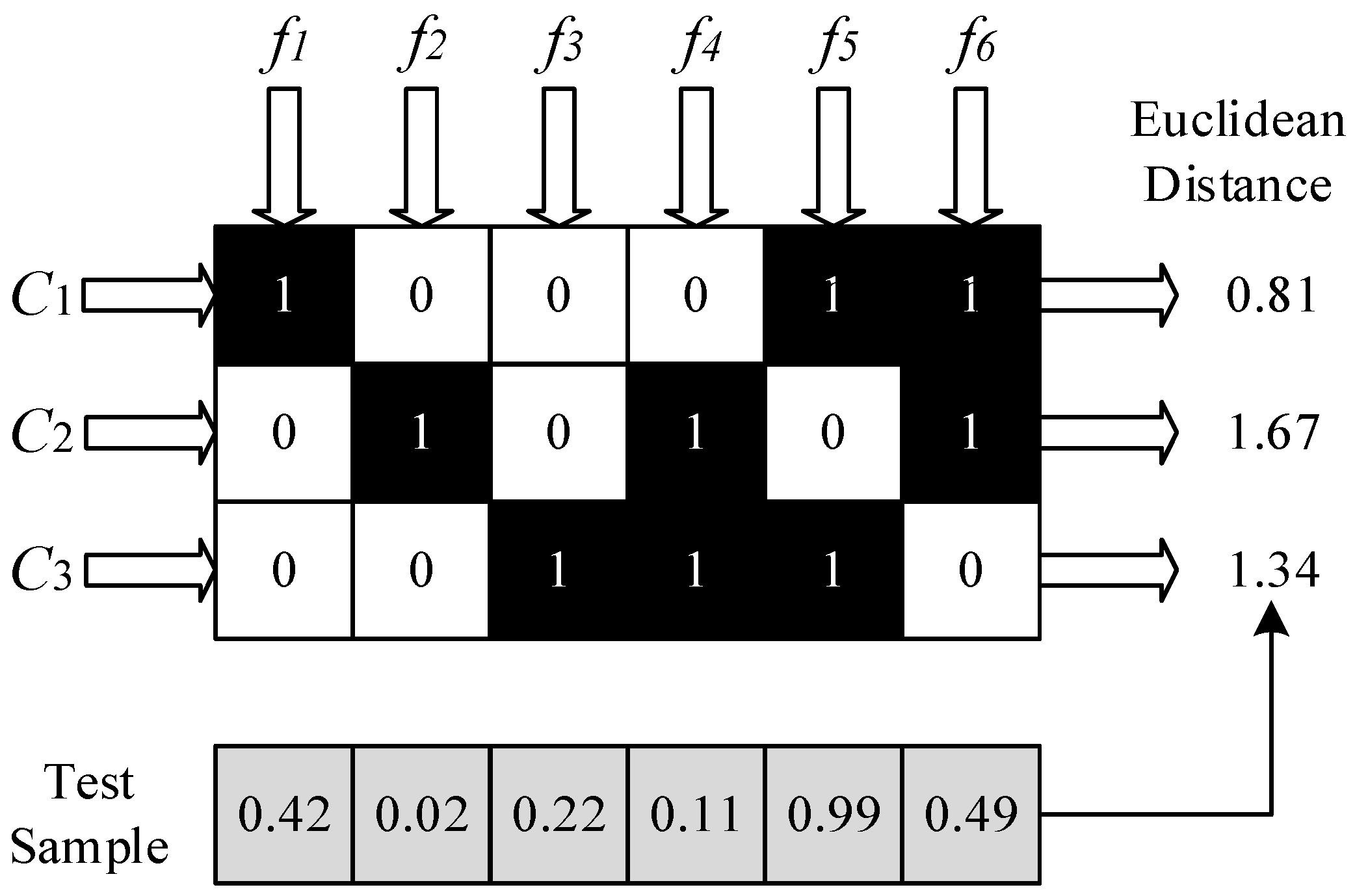
In traditional binary ECOC coding, the output of the binary classifier is either positive or negative. When a binary classifier faces a difficult-to-classify sample, its prediction probability tends to be near the middle value. This situation can easily cause the binary classifier to output random codes. Such random outputs can lead to misjudgments. Consequently, this affects the overall accuracy of the ECOC assessment. To address this issue, the paper proposes an improved error-correcting output code (I-ECOC) algorithm. This algorithm changes the output of the binary classifier to the corresponding prediction probability. And the prediction probabilities output by each binary classifier form the prediction code of I-ECOC. When a binary classifier faces a difficult-to-classify sample, its output prediction probability is closer to the middle value. This makes the classifier’s output approximately equidistant to each category. Thus, the influence of this classifier on the overall distance calculation can be disregarded. This significantly reduces the negative impact of the binary classifier on the overall assessment of I-ECOC, enhancing the fault tolerance and accuracy of the classification assessment model.
For a certain test sample, the probabilities of binary classifiers
,
,
,
,
and
predicting it as the positive class are 0.42, 0.02, 0.22, 0.11, 0.99, and 0.49, respectively. Using Equation (10) for calculation, the Euclidean distances of the test sample from categories
,
, and
are 0.81, 1.67, and 1.34, respectively. Therefore, the test sample can be classified as belonging to category
, as specifically shown in
Figure 5.
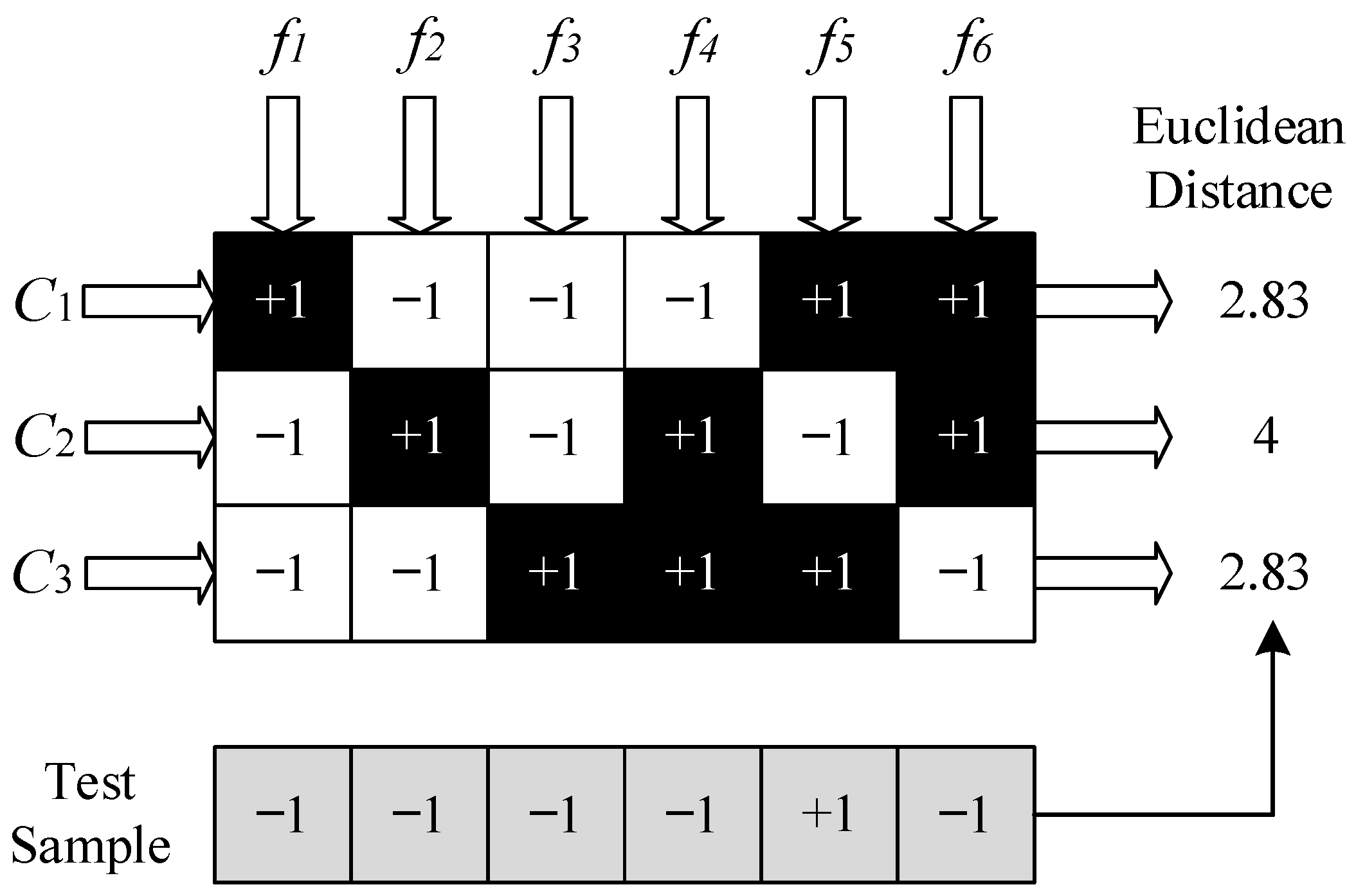
If the above test sample is evaluated using the ECOC method, the judgment process is shown in
Figure 6. Because binary classifiers
and
both make mistakes when facing difficult-to-classify samples, it leads to equal Euclidean distances from the prediction code to
and
. The assessment category of the test sample will be randomly chosen between
and
, which can easily lead to misjudgment.
2.5. Dataset Construction and Instability Discrimination Criteria
2.5.1. Dataset Construction
To address the issue of sample imbalance in the analysis of transient stability in power systems, the paper proposes using the CLV-GAN algorithm to enhance both aperiodic unstable samples and oscillatory unstable samples. This approach aims to balance the number of positive and negative class samples in the dataset. The dataset used for training binary classifiers
to
is shown in
Table 1.
2.5.2. Instability Discrimination Criteria
The criterion for determining whether a sample is stable is based on the transient stability index (TSI) [
23]. When the TSI is greater than 0, the power system is stable; when it is less than 0, the power system is unstable.
where
represents the maximum value of the rotor angle difference between two generators.
The definition of transient stability according to IEEE (Institute of Electrical and Electronics Engineers) [
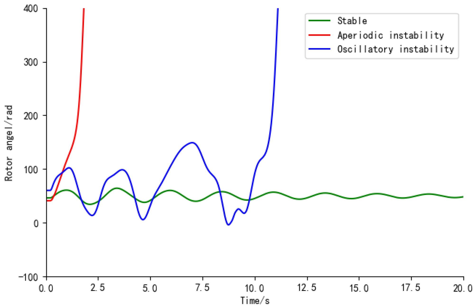
24] is: Due to insufficient synchronous torque, instability usually appears in the form of aperiodic angular separation, namely aperiodic instability. Unlike aperiodic instability, oscillatory instability is caused by insufficient damping torque among other reasons, with increasing amplitude. The rotor angle curves of the three modes are shown in
Figure 7. The horizontal axis represents the time after the power system experiences a disturbance, and the vertical axis represents the change in relative rotor angle after the disturbance.
Figure 7 clearly shows significant differences between the two instability modes. They have different leading causes and require different control measures. Therefore, accurately identifying different instability modes is of great importance for the safety of the power system.
2.6. Transient Stability Assessment Framework
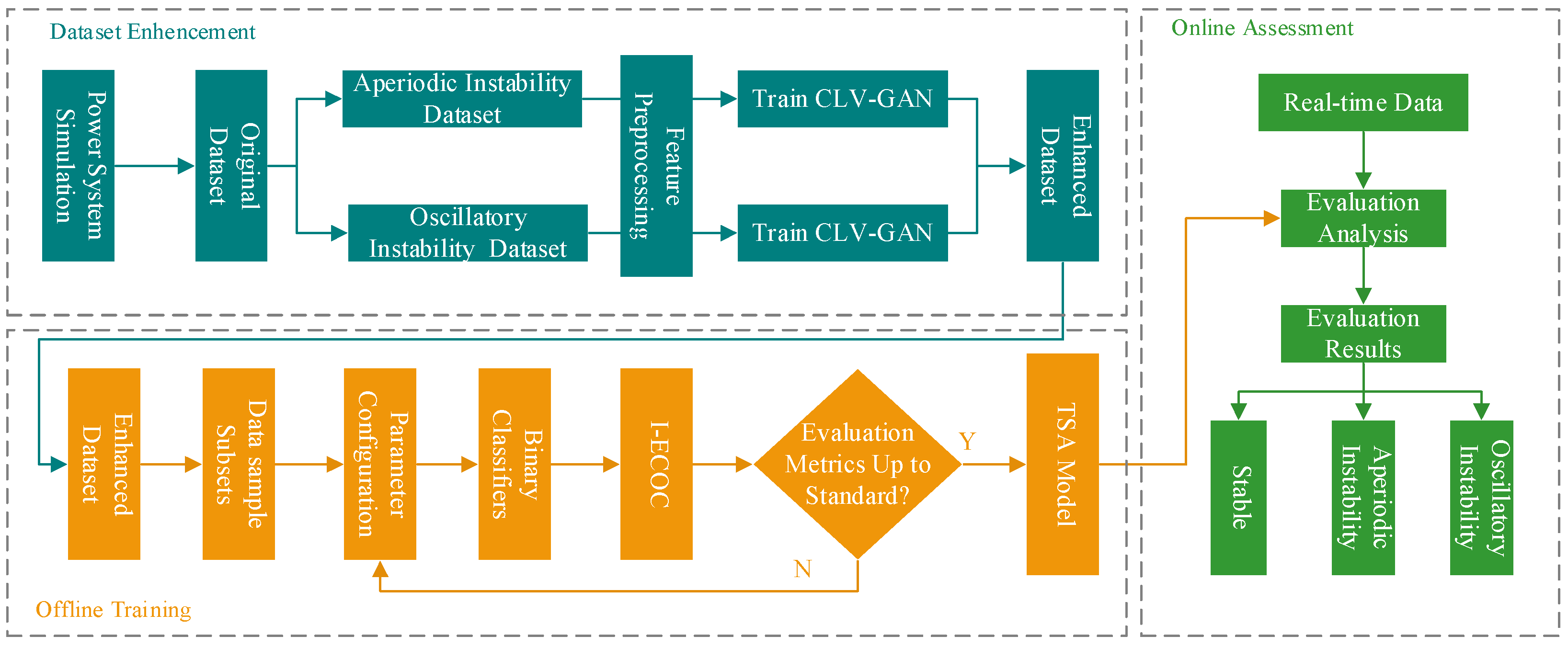
The framework of multi-class transient assessment model based on I-ECOC encoding is shown in
Figure 8. It mainly comprises three parts: dataset enhancement, offline training, and online assessment.
- (1)
Dataset Enhancement
Step1: Set up power system faults under different conditions to obtain the original dataset through simulation. The dataset contains three types of samples, stable, aperiodic unstable, and oscillatory unstable, with their corresponding labels being 0, 1, and 2, respectively.
Step2: Perform spatiotemporal feature preprocessing on the aperiodic unstable and oscillatory unstable samples in the dataset. Train the respective CLV-GAN data augmentation models with the processed data from the two types of instability.
Step3: Train the CNN classifier with the original data. Evaluate the synthetic data using the trained CNN, select the set of synthetic data with the best evaluation metrics, and add it to the original dataset to obtain an enhanced dataset.
- (2)
Offline Training
Step1: Divide the enhanced dataset into different data sample subsets as per
Table 1. Set the parameters for the binary classifier
, and train binary classifiers on different subsets. Adjust the parameters of the binary classifiers according to evaluation metrics to optimize the performance of each classifier on its corresponding data sample subset.
Step2: Compose the trained binary classifiers into an I-ECOC multi-class model according to the order of binary classifiers in the encoding matrix. If the I-ECOC model’s overall evaluation metrics on the test set meet the standards, the assessment model is outputted. If not, the optimization of the parameters and structure of the binary classifiers continues.
Step3: Select the I-ECOC model with the best evaluation metrics as the multi-class assessment model for power system transient stability, and apply it to online assessment.
- (3)
Online Assessment
Step1: Send real-time measurement data obtained from PMUs to the assessment model for evaluation and analysis to determine if the power system will become unstable and the type of instability.
3. Simulation and Discussion
To evaluate the effectiveness of our proposed method, we conducted simulation experiments on the IEEE 39-bus and IEEE 140-bus systems. The power system simulation software was PSD-BPA 3.07 from the China Electric Power Research Institute.
The operating condition parameters of the power system were set as follows:
- (1)
The case study considered nine load levels at 80%, 85%, …, 115%, 120%, with corresponding adjustments in generator output to maintain power system balance;
- (2)
The fault type was set as the most severe three-phase short-circuit fault in the power system, with fault locations set at 0, 10%, 20%, …, 90% of each line;
- (3)
The fault occurred at 0 s, and the fault was cleared after 0.1 s, 0.15 s, 0.18 s, and 0.2 s;
- (4)
The total simulation duration was 10 s, with a simulation step of 0.01 s. Data from 12 cycles after fault clearance were collected.
Bus voltage was the system’s load flow data and responded more quickly to faults than rotor angles [
25]. It accurately reflected the operating conditions of the system and could be measured by PMUs [
26]. Therefore, this paper used the bus voltage magnitude after fault clearance to construct the input feature set for the model.
For the IEEE 39-bus system, 12,240 samples were obtained through simulation, including 8123 stable samples, 3042 aperiodic unstable samples, and 1075 oscillatory unstable samples. For the IEEE 140-bus system, 22,140 samples were obtained through simulation, including 16,858 stable samples, 3853 aperiodic unstable samples, and 1429 oscillatory unstable samples. And the data were divided into training and test sets at a ratio of 7:3.
3.1. Performance Evaluation Metrics
The paper analyzed the performance of the transient stability multi-class assessment model using overall assessment accuracy
, oscillatory instability assessment accuracy
, and comprehensive indicator
. The confusion matrix is shown in
Table 2.
where
represents the proportion of stable samples correctly predicted out of all stable samples;
represents the proportion of aperiodic unstable samples correctly predicted out of all aperiodic unstable samples;
represents the proportion of oscillatory unstable samples correctly predicted out of all oscillatory unstable samples; and
is the geometric mean of the above three indicators.
3.2. CLV-GAN Performance Evaluation
To verify the effectiveness of the CLV-GAN generation algorithm, it was compared with three commonly used generation algorithms: synthetic minority oversampling technique (SMOTE) [
27], adaptive synthetic sampling (ADASYN) [
28], and deep convolutional GAN (DCGAN) [
29]. The number of artificial samples generated by the four generation algorithms was equal to the difference between the number of stable samples and aperiodic unstable samples, as well as the difference between the number of stable samples and oscillatory unstable samples. The classification model used for testing was a CNN, and it used an architecture with 3 convolutional layers and 3 fully connected layers, with a training duration of 150 epochs and an Adam learning rate of 0.001. The experimental results are shown in
Table 3 and
Table 4.
In the original unbalanced dataset, as can be seen from
Table 3 and
Table 4, the value of
was much greater than the value of
. Therefore,
was no longer a good metric to evaluate the performance of classification models in unbalanced datasets and the value of
needed to be taken into account as well. In the IEEE 39-bus system, the values of
,
, and
in the CLV-GAN dataset increased by 10.62%, 5.92%, and 1.22%, respectively, compared to those in the original dataset. In the IEEE 140-bus system, the values of
,
, and
in the CLV-GAN dataset increased by 8.97%, 5.49%, and 0.79%, respectively, compared to those in the original dataset. In both power systems, the value of
for CLV-GAN was higher than that of other comparison algorithms. This demonstrated the performance of the CLV-GAN algorithm, but we also realized that this method has a potential shortcoming. It is that our method has a relatively high computational complexity, which may limit its application in resource-limited environments. To overcome this shortcoming, we will strive to optimize the algorithm to reduce computational complexity.
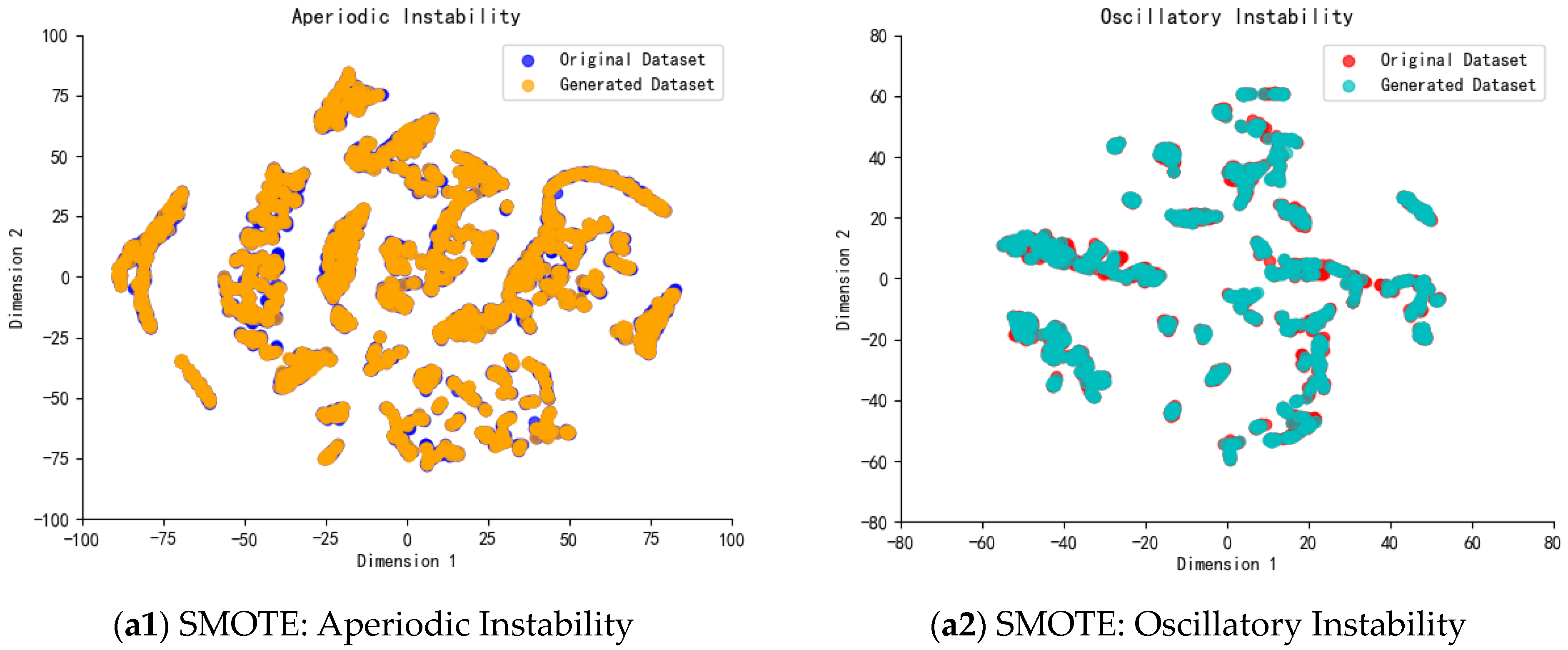
To further analyze the effects of different data augmentation algorithms, the synthetic samples from each algorithm were reduced to a two-dimensional plane for visualization using the t-distributed stochastic neighbor embedding (t-SNE) tool [
30]. From
Figure 9, it can be seen that the SMOTE algorithm generated new samples randomly along the lines connecting similar and neighboring minority samples, based on the proportion of differences between minority and majority samples. The ADASYN algorithm determined the number of samples to be generated based on the number of stable samples surrounding the unstable samples. The DCGAN and CLV-GAN algorithms both learned the latent distribution from real samples and generated new samples from this latent distribution. However, as can be seen from
Figure 9, the distribution of data generated by CLV-GAN was closer to the distribution of real data than that generated by DCGAN. In summary, the above simulations verified the effectiveness of the CLV-GAN algorithm proposed in this paper, which can effectively alleviate the harm caused by sample imbalance to the multi-class assessment model.
3.3. I-ECOC Performance Evaluation
To verify the effectiveness of the proposed multi-class model, it was compared with four multi-class models: ECOC, CNN, support vector machine (SVM) [
31], and random forest (RF) [
32]. In the I-ECOC model, the training rounds for each binary classifier were set to 150 epochs, with an Adam learning rate of 0.001 for all. For SVM, the kernel function was the radial basis function, gamma was set to scale, and penalty parameter C was set to 1. RF integrated 50 trees for learning. CNN used an architecture with 3 convolutional layers and 3 fully connected layers, with a training duration of 150 epochs and an Adam learning rate of 0.001. The hyperparameters of the ECOC model were kept consistent with those of the I-ECOC model. The comparative experiments used two sets of datasets, before and after enhancement, with each dataset divided into a training set and a test set in a 7:3 ratio. The simulation results on the IEEE 39-bus and IEEE 140-bus systems are shown in
Table 5.
Table 5 shows the performance of I-ECOC and four other comparison models on four datasets. As can be seen from
Table 5, the
value of I-ECOC outperformed other comparison models in the original dataset. For the IEEE 39-bus system, the
value of I-ECOC was improved by 7.20% and the
value was improved by 0.44% compared to ECOC in the original dataset. For the IEEE 140-bus system, the
value of I-ECOC was improved by 3.66% and the
value was improved by 0.13% compared to ECOC in the original dataset. It fully validated the performance of the proposed I-ECOC model in the transient stability assessment of power systems. At the same time, we can also conclude that the data augmentation algorithm mainly improved the recognition accuracy of minority classes.
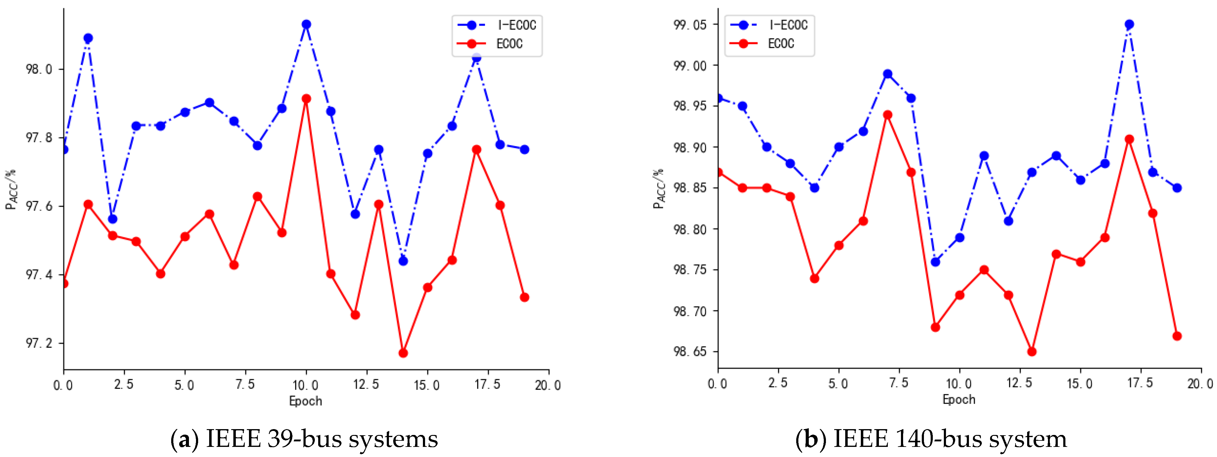
To further verify the effectiveness of the improvements made to I-ECOC, 20 rounds of tests were conducted on both the IEEE 39-bus and IEEE 140-bus systems for the I-ECOC and ECOC models. The datasets used in the 20 rounds of testing were all original datasets. The test results are shown in
Figure 10.
In
Figure 10a,b, the horizontal axis represents the round of testing and the vertical axis represents the testing accuracy
. And the blue curve represents the I-ECOC model and the red curve represents the ECOC model. In the 20 rounds of tests, as can be seen from
Figure 10, the
of the I-ECOC model was always superior to that of the ECOC model. It once again validated the improvement of the I-ECOC model compared to the ECOC model, but there are still some disadvantages that cannot be ignored. The parameter tuning process of the I-ECOC model is relatively cumbersome, requiring a lot of time and effort for debugging. Secondly, the generalization ability of the model in some specific scenarios will need to be improved. For example, the distribution of input data will also change when the topology of the power system changes. And it may lead to fluctuations in the model’s performance. To improve these aspects, we will further simplify the process of model parameter tuning and explore more effective regularization methods to enhance the generalization ability of the model.
3.4. Noise Resistance Performance Analysis
According to the IEEE standard for synchronized phasor data transmission in power systems, PMU phasor measurement units will have a measurement error of less than 1% [
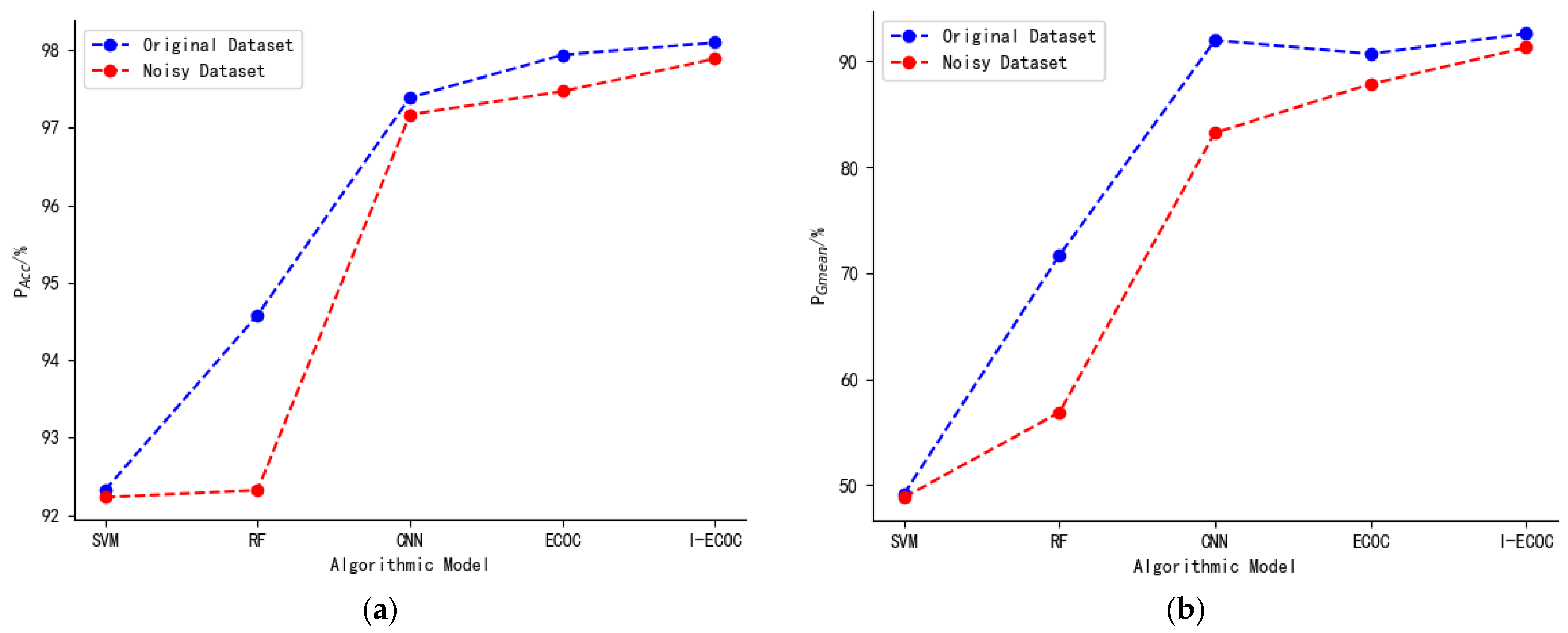
33]. To verify the robustness of the I-ECOC model, random measurement noise within the range of −1% to 1% was added to each sampling point in the test data. Under conditions of noise interference, the assessment performance of each model is shown in
Figure 11.
In
Figure 11a,b, the horizontal axis represents the type of evaluation model, and the vertical axis represents the
and
of each model. In
Figure 10, the blue curve represents the original dataset and the red curve represents the noisy dataset. From the test results in
Figure 11, it can be seen that the performance of all assessment models decreased under noise interference. However, compared with other assessment models, the
and
of the I-ECOC model remained the highest. Meanwhile, under noisy interference, the declines in both the
and
of the I-ECOC model were less than the declines seen in the ECOC model. It fully demonstrated the robustness of the I-ECOC model.
4. Conclusions
Due to the characteristics of safe operation of power systems, there is a serious imbalance in the proportion of stable operation samples to unstable samples. Previous studies did not consider the spatiotemporal characteristics of power system samples when supplementing unstable samples. Therefore, there are some deviations between the generated samples and the real samples. It leads to weaker generalization ability of the trained model. In addition, most of the existing research on transient stability models for power systems focuses on binary classification problems, neglecting the situation where oscillatory unstable samples are easily misclassified as stable samples. In addition, most of the existing research on TSA primarily focuses on binary classification problems, overlooking the situation where oscillatory unstable samples are often misclassified as stable samples. It poses significant hidden dangers to the safety of power systems. This paper makes a thorough study on these two aspects and proposes a multi-classification assessment model for power system transient stability based on CLV-GAN and I-ECOC. Simulation analysis was conducted on the IEEE 39-bus and IEEE 140-bus power systems, leading to the following conclusions:
- (1)
After fully considering the spatiotemporal characteristics of power system data samples, we propose a data enhancement algorithm CLV-GAN based on spatiotemporal features. The algorithm improves VAE by introducing modules for temporal and spatial feature extraction and makes the distribution of the generated samples closer to the distribution of real samples. It effectively mitigates the harm caused by sample imbalance. At the same time, it also improves the reliability of the model and increases the recognition accuracy for minority class samples.
- (2)
When utilizing the ECOC encoding strategy to solve multi-classification problems, the algorithm is prone to errors with borderline samples. Therefore, we propose an improved ECOC algorithm. It improves the output and encoding–decoding methods of the binary classifiers in ECOC. It reduces the impact of errors in the binary classifiers’ judgments of borderline samples and enhances the fault tolerance of the model.
- (3)
Regarding the issue of noise interference during data collection and transmission, we conducted simulation analysis by adding random noise ranging from −1% to +1% to the dataset. The simulation results fully demonstrated that the assessment model proposed in this paper has good robustness.
Because the computational complexity and the number of parameters of the improved algorithm proposed in this paper are both very high, in the future, we will strive to optimize the algorithm to decrease computational complexity and reduce the number of parameters to make the model lighter. When the topological structure of the power system changes, the distribution of data will also change accordingly. It can lead to a significant decrease in the performance of the evaluation model. Therefore, quickly improving model performance under changing data distributions is also a future research direction.


