Abstract
Accurate electricity demand forecasting is essential for global energy security, reducing costs, ensuring grid stability, and informing decision making in the energy sector. Disruptions often lead to unpredictable demand shifts, posing greater challenges for short-term load forecasting. Understanding electricity demand patterns during a pandemic offers insights into handling future disruptions. This study aims to develop an effective forecasting model for daily electricity peak demand, which is crucial for managing potential disruptions. This paper proposed a hybrid approach to address scenarios involving both government intervention and non-intervention, utilizing integration methods such as stepwise regression, similar day selection-based day type criterion, variational mode decomposition, empirical mode decomposition, fast Fourier transform, and neural networks with grid search optimization for the problem. The electricity peak load data in Thailand during the year of the COVID-19 situation is used as a case study to demonstrate the effectiveness of the approach. To enhance the flexibility and adaptability of the approach, the new criterion of separating datasets and the new criterion of similar day selection are proposed to perform one-day-ahead forecasting with rolling datasets. Computational analysis confirms the method’s effectiveness, adaptability, reduced input, and computational efficiency, rendering it a practical choice for daily electricity peak demand forecasting, especially in disrupted situations.
1. Introduction
Accurate and practical forecasting is essential for planning purposes in any industry. In the electric utility industry, it involves generating demand forecasts to prepare for future electricity requirements and ensure adequate resources are available to meet future demand [1]. The problem of increasing fluctuations in electricity demand brings global attention to the electric utility industry [2,3]. Understanding how emergencies can impact the power industry, and effectively managing energy distribution, make it important to focus on power industry [4]. Accurate forecasting is essential for helping the utility industry to determine load scheduling, power storage reserve, and facility layout, leading to overall improvements in these areas [5,6].
Over the past few years, nations worldwide have prioritized environmental sustainability and a shift toward renewable energy, recognizing these as critical global concerns [7]. The utilization of renewable energy sources is crucial in the global economy due to their substantial impact on reducing environmental pollution, aligning with efforts to address climate change and decrease CO2 emissions. Sustainable production and consumption patterns play a key role in tackling climate change by reducing energy consumption and transitioning to less carbon-intensive energy sources; these are essential steps toward achieving a low-carbon economy and ensuring climate stability [8,9]. As highlighted in numerous recent studies [10,11,12], renewable energy stands at the forefront of globalization processes and the energy transition. As nations worldwide increasingly emphasize sustainability, renewable energy emerges as a leading force driving this transformative shift. The widespread adoption and innovation of renewable energy contribute significantly to shaping a more interconnected and sustainable energy landscape on a global scale. Accurate electricity forecasting is one of the keys to reducing environmental impact and increasing sustainability. It offers precise insights into future energy demand, enabling optimized generation strategies. Accurate forecasting helps with efficient resource allocation, reducing wastage in energy production. Additionally, it ensures a balanced supply-demand equilibrium, preventing grid failures or overloading, which could harm the environment. Moreover, precise forecasting empowers consumers and industries to adopt energy-efficient practices, contributing to better resource management and a more sustainable energy landscape, which are all pivotal in mitigating environmental impact.
In addition, during disrupted situations, power consumption may experience significant fluctuations. Due to intervention from government policies, such as lockdowns and restrictions, the closure of nonessential businesses and stay-at-home restrictions have resulted in significant shifts in both magnitude and daily demand patterns [13]. The sudden and dramatic changes in consumption patterns have brought challenges in short-term load forecasting, as forecasting algorithms were not equipped to anticipate such unprecedented shifts in human behaviors regarding power usage. Since disrupted situations fundamentally invalidate the forecasting assumption that future demand follows historical patterns, the lack of historical data from such unprecedented events of extreme disruptions makes it difficult for traditional models to accurately predict the impact on electricity demand [14]. Understanding the electricity demand pattern during a pandemic can provide additional insights into how the electric utility industry will respond to future disrupted situations.
Due to the worldwide impacts of COVID-19, electricity demand data during this event are used as a case study to represent disrupted situations in this work. The COVID-19 pandemic had a rapid and negative impact on many sectors across the world within a short period [15,16,17]. Among these affected industries, the energy sector was one of the most affected [17]. Focusing on its effect on the energy sector, Aktar, Alam, and Al-Amin [18] conducted a review study to identify the impacts of the COVID-19 pandemic on energy demand, CO2 emissions, and the economy. To assess the short-term and long-term impacts on energy use within households, the effects of COVID-19 on household energy consumption were examined by Cheshmehzangi [19]. Abulibdeh, Zaidan, and Jabbar [20] studied the impact of the pandemic on electricity demand and electricity demand forecasting accuracy. After the impacts on electricity demand forecasting are demonstrated, an accurate forecasting performance is a goal that many researchers try to achieve.
In the electricity demand forecasting problem, statistical techniques and machine learning techniques are the two main techniques that are frequently used, not only in normal situations but also in the COVID-19 pandemic situation. In normal situations, the statistical linear regression model [21,22] is the most commonly applied method due to its simplicity and interpretability. Additionally, more advanced forecasting techniques, such as the autoregressive integrated moving average model (ARIMA) [23], ARIMA with exogenous variables (ARIMAX) [24], and grey model [25] are also frequently employed.
During the COVID-19 pandemic situation, significant attention was given to adaptability to changes in consumption patterns. Advanced techniques were also used in the pandemic situation. Alasali et al. [26] applied ARIMAX to minimize the pandemic’s impact on forecasting models, focusing on long-term electricity demand trends. Similarly, Huang et al. [27] enhanced predictive capabilities by combining rolling mechanisms with the grey model to utilize the latest acquired data. However, a single advanced model is not sufficient to handle specific conditions, leading to the introduction of hybrid models. In a situation where exogenous variables were not available, a hybrid model of generalized additive models (GAM) and Kalman filtering was applied to enhance adaptability [28]. To deal with limited data during the pandemic situation, a hybrid model of fractional grey prediction models with genetic algorithm (GA) optimization was successfully applied to forecast monthly electricity generation data [29]. However, statistical techniques have limitations in capturing non-linear patterns that appear in the recent electricity demand trend [30]. To overcome this limitation, machine learning techniques are applied to the electricity demand forecasting problem. With continuous learning capabilities, machine learning algorithms provide real-time updates as consumption patterns change during disrupted situations, making them well suited for dynamic and changing forecasting scenarios [31].
Due to its several advantages, machine learning has become widely applied in electricity demand forecasting. Popular machine learning models such as support vector machines (SVM) [32], the artificial neural network (ANN) [33], and long short-term memory (LSTM) networks [34] are utilized in this area. To enhance the efficiency of managing uncertainty occurring in forecasting tasks, a combination of statistical and machine learning techniques has been introduced. Bayesian regularization, based on the Gaussian process [35], is applied to incorporate uncertainty into the forecasting process. This approach is particularly valuable for scenarios involving complex and limited available data. Machine learning models are not commonly applied to electricity demand predictions during normal situations but have been adapted to handle the unique challenges caused by the COVID-19 pandemic situation. Sozen et al. [36] applied LSTM to forecast daily electricity demand in the early stage of the COVID-19 pandemic. With a simple structure, and easy to implement in a practical system, ANN was used to forecast electricity demand during the pandemic [14]; however, training ANN with the standard input variables, such as weather conditions and previous consumption levels, might not give satisfactory results. Chen, Yang, and Zhang [14] improved ANN forecasts using economic activity-based mobility data; however, without sensitivity factors representing the pandemic situation, a hybrid model of improvement techniques should be performed to increase the accuracy of the simple-structured machine learning models. A hybrid LSTM model with simplex optimizer [37], and with grid search and manual search [38], is applied to improve performance through hyperparameter tuning. To enhance SVM performance, a hybrid model of the data decomposition technique called improved complete ensemble empirical mode decomposition with adaptive noise (ICEEMDAN), and the multi-objective grey wolf optimizer (MOGWO), is employed [39]. Additionally, the integration of a transfer learning framework with neural networks can glean insights into exogenous variables’ impact on pandemic electricity consumption [40]. The summary technique used in previous research during the COVID-19 pandemic is shown in Table 1.

Table 1.
The summary technique used in previous research during the COVID-19 pandemic.
Based on the previous research presented in Table 1, two gaps have been identified in the literature during the COVID-19 pandemic. The first gap lies in the integration and development of models specifically designed for hybrid scenarios that blend elements of both lockdown and non-lockdown situations. While existing models excel in predicting demand under normal conditions or during strict lockdowns, there is a lack of comprehensive frameworks capable of adapting to transitional phases, where restrictions fluctuate or are gradually relaxed. The second gap involves the hybrid model aiming to incorporate four intriguing techniques identified in the COVID-19 literature. The first technique is data decomposition. Without applying this method, the forecasting model loses seasonal and trend information, increasing difficulty in handling seasonal patterns. Consequently, inaccurate forecasting results are produced, especially in long-term forecasting, as the model is unable to capture underlying patterns. The second technique is selecting input variables. Neglecting this process may introduce irrelevant or redundant variables into the model, leading to overfitting issues that reduce the efficiency of the forecasting model. Moreover, it increases model complexity and consumes computational resources and time. The third technique is hyperparameter optimization. Without utilizing this method, an overfitting and underfitting problem can be created due to the improper hyperparameter setting leading to the reduction of forecasting performance. Besides, it increases the risk of bias when selecting hyperparameters manually. The fourth technique is presented in the rolling dataset. In the pandemic situation, where the situation changes daily, adjacent data is important as it contains the current state. Fixed training datasets limit adaptability and reduce the robustness of the forecasting model, leading to poor forecasting results. Integrating these techniques into a hybrid model seeks to mitigate these drawbacks and enhance the accuracy, adaptability, and robustness of the forecasting approach amidst the complexities of COVID-19-induced fluctuations and transitions.
However, a specific model designed for hybrid scenarios, along with the combination of data decomposition, input variable selection, hyperparameter optimization, and a rolling dataset, has never been applied to the pandemic situation. With a combination of these methods, the problems of adapting to the transitional phase, capturing underlying seasonality patterns, overfitting, and the complexity of the model can be solved by the proposed model. Furthermore, the proposed approach utilizes the latest acquired data by rolling dataset as well as preventing performance bias related to hyperparameters. Additionally, to the best of the authors’ knowledge, this hybrid approach is the first in the existing literature proposed specifically for disrupted situations in Southeast Asia.
When considering methods for enhancement, data decomposition is considered as a technique to significantly improve the accuracy of forecasting electricity demand. This technique is applied to the time series data for separating linear and non-linear components from the original data [41]. Traditional data decomposition methods such as discrete wavelet transform (DWT), and empirical mode decomposition (EMD), are commonly used in various fields. DWT decomposes the original data into low-pass components (approximations) and high-pass components (details) by dilating, scaling, and translating the original data to cover the wavelet filter. However, DWT has limitations related to the discrimination effect, and its performance depends on expert decisions regarding the choices of wavelet filter and levels of decomposition [42]. To overcome the limitations of DWT, EMD was introduced as an alternative that offers the advantage of automatically decomposing the original data based on the data characteristics, which eliminates the need for expert decisions [43]. EMD decomposes the original data into intrinsic mode functions (IMFs) and residuals. It uses a sifting process to identify modes by analyzing the envelope’s minima and maxima. However, when the number of extrema is abnormal, EMD faces a mode mixing issue, where a mode cannot be isolated into a single IMF and ends up mixed within another IMF [44]. Ensemble empirical mode decomposition (EEMD) is the method designed to solve the issue of the mode mixing effect present in EMD by adding white noise to the original data; however, the addition of white noise creates an endpoint effect problem, leading to distortion. Furthermore, the additional white noise increases the noise and complexity of the original data, leading to a new problem of generating a varying number of IMFs in each iteration [45]. Variational mode decomposition (VMD) represents an improvement over EEMD as it effectively solves the problems of mode mixing, endpoint effect, and varying numbers of IMFs [46]. In the case of enhanced VMD capabilities, Jiang et al. [47] focused on applying fast Fourier transform (FFT) to adjust seasonal patterns. Seasonal patterns capture the regular and predictable fluctuations that occur in electricity demand over specific periods. By including these patterns, the forecasting model can better capture the underlying trends and produce more accurate predictions. However, determining the optimal decomposition level for VMD remains an open challenge that researchers are actively working on. Defining a suitable decomposition level for VMD becomes even more challenging when dealing with intricate non-linear and non-stationary elements in the original data. Multiple time series data components will coexist in one mode if the decomposition level is set too low. On the contrary, setting the decomposition level too high will lead to one component of the time series data being present in multiple modes, causing potential mixing and ambiguity in the decomposition results [48]. Optimization techniques are commonly applied to determine the optimal decomposition level [49,50,51]; however, optimization techniques have general drawbacks, including the challenges of finding global solutions and the complexity of implementing intricate optimizers [52]. When dealing with complex problems, many iterations are required to search for the optimal solution, resulting in significant computational time and resources. To overcome these limitations, Aswanuwath et al. [53] proposed a novel approach by utilizing the suitable decomposition level obtained from EMD as a guide for defining the appropriate decomposition level in VMD. VMD-based EMD not only saves computational costs and time in the search for the optimal solution, but also ensures more efficient and accurate decomposition.
Input variables are another key factor that directly impacts the accuracy of the forecasting model. Determining the most useful inputs for the forecasting process can be one of the most critical decisions during the model development process. However, the set of candidate input variables usually includes variables that might be either irrelevant or redundant. Irrelevant inputs provide no informative value and only introduce noise and unnecessary complexity into the model. On the other hand, redundant inputs increase the model’s dimensionality without offering any additional predictive benefits. Meanwhile, neglecting relevant input variables results in an inaccurate forecasting model [54]. Input variables selection methods, such as search strategy-based input variable selection (IVS) algorithms [55], exhaustive search-based predetermined optimality criteria [56], heuristic search [57,58], and stepwise selection [59] are widely used for machine learning. Stepwise regression is considered an appropriate method due to its systematic approach and ease of verifying and explaining relationships between response variable(s) and candidate predictor variables. Recently, a similar day selection (SD) method has been introduced to the electricity demand forecasting field with the aim of training the model with historical input variables sharing characteristics similar to that of the target forecast date [60,61]. SD selects similar days by analyzing the similarity between the target forecast date and past dates [62]. In the case of external factors such as temperature humidity and wind speed on the forecast date being missing or unavailable, the SD method remains effective by using historical days with available data to make predictions. Furthermore, it reduces data complexity by considering all historical data points, leading to more efficient computations and faster forecasting. Several approaches have been considered to improve SD’s performance. These include incorporating timing information and external factors as input variables and employing enhancement techniques [63,64,65]. However, the previous works implementing SD neglect the significance of special days and do not include them in the forecasting model. Additionally, much of this research applies meteorological variables, such as temperature and humidity, as factors for selecting similar days. Since the actual meteorological variables are unknown in advance, the forecasting of meteorological variables is required. Senjyu et al. [66] provided evidence of increasing errors resulting from the use of weather forecast data as input variables. Existing gaps in past research contain the criterion for selecting input variables and the practical implementation of input variable selection techniques for a disrupted situation.
Due to the ongoing impact of disrupted situations such as the COVID-19 pandemic on the global energy sector, the aim of this work is to develop an accurate electricity demand forecasting model to manage a possible disrupted situation that might occur in the future. Based on the large economy of Thailand, which ranked as the eighth largest in Asia and the second largest in Southeast Asia according to the World Bank’s 2018 report [67], electricity demand data provided by the Electricity Generating Authority of Thailand (EGAT) can be used as a representative case study to develop a pandemic forecasting model.
In order to solve the problem of input variable selection and data decomposition, a hybrid approach of VMD-EMD-FFT, SD, stepwise regression, and ANN was proposed and successfully enhanced the accuracy of forecasts and saved computational time [53]; however, there are limitations when applying this model to the pandemic year. Specifically, the model lacks the flexibility and adaptability needed to quickly adjust to sudden changes when disrupted events occur. These limitations stem from the model’s method of incorporating historical data, which overlooked the different characteristics of the short-term dataset (the most recent data during the pandemic year), medium-term dataset (the encompassing data from an intermediate time span), and long-term dataset (the data before the pandemic year). Consequently, a significant portion of the training dataset originated from the normal situation phase, which failed to accurately represent electricity demand during disruptions. Moreover, the model’s SD strategy, which selected similar days based on the demand of the pre-pandemic year, is impractical because the demand in the year before the disrupted event reflects a standard situation phase and does not capture demand dynamics during disruptions. Thus, these limitations confine the flexibility of the forecasting model, making it hard to capture the intricate electricity demand patterns during disrupted situations, leading to poor forecasting outcomes.
The added value and key novelty of this paper are the integration of demand analysis and probabilistic load forecasting in the context of disrupted situations, considering new demand patterns and behavioral and cultural shifts. The main contributions encompass various aspects. Firstly, this paper contributes to the development of a forecasting model for hybrid scenarios during disruptions, utilizing a combination of techniques including VMD-EMD-FFT, SD, stepwise regression, ANN, LSTM, and GS optimization. This aims to expand the model’s flexibility while maintaining efficient computational processing, making it a practical choice for real-world applications. Secondly, it introduces a new criterion to separate short-term, medium-term, and long-term input sets for the context of disrupted situations. Additionally, it proposes a new SD criterion for handling a situation where the demand of a candidate date shows low similarity to the target date. Further, it enhances model adaptability for daily changes by performing one-day-ahead forecasting with rolling datasets and pandemic sensitivity factors, while avoiding input variables necessitating additional forecasting. Moreover, it evaluates the proposed approach with actual electricity demand data provided by EGAT. This paper also provides an understanding of the model’s performance in different scenarios, offering valuable guidance for decision making in diverse situations. It analyzes how disruptions affect the forecasting model’s accuracy as an external variable. Lastly, it focuses on improving forecasting accuracy during disrupted situations, reducing model input data, and saving computational time.
The rest of this paper is organized as follows: Section 2 introduces the overall procedure of the proposed model for the disrupted situation and the theoretical framework used in this work; Section 3 presents an electricity demand forecasting case study using the proposed model and its results; and Section 4 gives conclusions and directions for future work.
2. Methods
2.1. Overall Procedure of the Proposed Model for the Disrupted Situation
In the disrupted situation, the pattern of electricity demand fluctuates and dramatically changes, due to various external factors, including the impact of government policies and regulatory changes. These policies can highly impact the daily lives of people, leading to shifts in energy consumption patterns and accessibility to essential services. Consequently, the model needs to be sufficiently adaptive and flexible to accommodate the immediate changes in demand caused by disrupted events and shifts in government policies. To ensure the forecasting model can adapt to these changes, training the model with different datasets, which contain different characteristics of time frames, is necessary. The short-term input set comprises the most recent data used to train the pattern of the data during the disrupted situation, while the medium-term input set, encompassing data from an intermediate time span, provides additional insights for the model to analyze transitional patterns between the disrupted and normal stages. Additionally, the long-term input set consists of historical data that allows the model to learn the pattern of the normal stage.
The proposed model is constructed by mainly focusing on the intervention of government policy, as shown in Figure 1. As shifts in consumption patterns related to government policy constitute a unique pattern not encountered in the past, the period under this situation needs to be treated differently from a disrupted situation without government interference. To enable the forecasting model to adapt to this change, a short-term input set containing the data adjacent to the target date is used to train LSTM, which is recognized for its adeptness in capturing and learning from temporal dependencies.
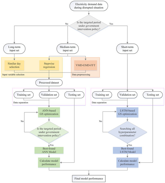
Figure 1.
Architecture of the proposed model for the disrupted situation.
However, if the target period is not influenced by government intervention policies, the electricity consumption indicates a combination of disrupted and normal patterns. To accommodate these fluctuations, medium-term and long-term input sets are utilized in the training of ANN. For identifying the hidden seasonality and trend of the disrupted situation presented in the medium-term period, VMD-EMD-FFT is used for data decomposition, seasonality, and trend identification. In addition, to identify the date during the normal stage that shares similarities with the target date during the disrupted stage, an SD with day type criterion is applied to select the date in the long-term period that is most similar to the target date, with a primary focus on the day types. With the purpose of reducing the computational cost for the forecasting model, the significant input variables of long-term and medium-term input sets are selected using SD and stepwise regression, respectively.
The short-term input set, along with the processed dataset resulting from input variable filtering and data preprocessing, is split into training, validation, and testing sets simultaneously, with overlapping data points (rolling dataset). To make the forecasting model adaptable to changes occurring during disrupted situations, one-day-ahead forecasting is applied to the proposed model. The training and validation sets are used in grid search optimization to tune hyperparameters for both ANN and LSTM. After searching through all hyperparameter combinations, the best-found model is applied to the testing set to calculate the model’s performance and evaluate the final performance of the forecasting model in the disrupted situation. The concepts and details of the proposed methods are described in Section 2.2, Section 2.3 and Section 2.4.
2.2. Input Variable Filtering
When applying neural networks to real-world problems, one of the critical concerns lies in the selection of input variables [68]. Choosing the appropriate inputs for forecasting is crucial in model development. The set of candidate variables may include irrelevant or redundant factors. Irrelevant inputs add noise and complexity, while redundant ones increase model size without improving predictions. Meanwhile, neglecting relevant inputs can lead to inaccuracies in forecasting [54]. The aim of input filtering contains three main objectives: enhancing model performance, reducing computational time, and providing deeper insights into the underlying data generation process [69].
In this section, the input variable filtering contains two methods, which are stepwise regression and SD. SD is applied for selecting the most similar date by using day type as a criterion. The stepwise regression method is used for selecting the significant input variables from the variables related to date and daily electricity demand.
2.2.1. Input Variable Description
The input variables used for stepwise regression are generated from two types of variables: date and electricity demand. The generated input variables serve as candidate input variables for selection through the stepwise regression process. The generated inputs related to date include binary index variables representing the day of the week (Monday–Sunday) and binary index variables representing special holidays. The generated inputs related to the historical electricity demand consist of variables with the lagged value from 1 day () to 7 days (), lagged daily electricity demand to moving average weekly and monthly index variables (), and moving average index variables with lagged period (), starting from to . is used to identify and quantify regular patterns that repeat at fixed intervals within a time series, while is applied to present the underlying trends and reduce the impact of short-term fluctuations or noise in the data. The mathematical expressions to generate and are as follows:
where represents lagged daily electricity demand to moving average index; represents daily electricity demand at period t; N is the length of the day for computing ; p is the number of lagged periods; and is the length of the day for computing . In order to compute weekly LMA and monthly LMA, L is set equal to 7 days and 30 days, respectively. For computing to , P is set equal to 2 days to 7 days.
2.2.2. Stepwise Regression
Regression analysis is a statistical method for examining the relationships between variables. It is commonly used to determine the causal effect of one variable on another [70]. Among statistical methods, multiple regression analysis is the most frequently used to examine the relationship between a single dependent variable and several independent variables [71]. A high correlation value indicates a strong linear relationship between the explanatory variables and the response variable, whereas a low correlation score implies a weak relationship. The multiple regression model can be written as:
where represents the response variable or the predicted value of the dependent variable; represents independent or predictor variables (i = 1, 2, …, p); represents the value of when all of the independent variables are equal to 0; represents the estimated regression coefficients (i = 1, 2, …, p); represents a random error component; and P represents the total number of independent variables.
Stepwise regression is an effective statistical method usually used to increase the regression model’s accuracy [72]. The main objective of stepwise regression is to choose the significant regressors from a large pool of possible ones, considering only the regressors that have an independent effect on the dependent variable [73]. In stepwise regression, there are three approaches used for selecting the model: call forward selection, backward selection, and bidirectional elimination [74]. Forward selection starts with an empty model and then adds the variable that will most significantly improve the model one at a time, until no other added variables can significantly improve the model. On the other hand, backward selection starts with a full model that includes all candidate input variables and then removes the variables that have the least potential to improve the model one at a time, until no more deleted variables can significantly improve the model. Bidirectional elimination is the combination of forward and backward selection. This selection approach is usually used when the correlations between variables exist in the model.
In this study, the bidirectional elimination criteria are α-to-enter and α-to-remove, both set to 0.1. From a statistical testing standpoint, the significance level (or type I error) represents the probability of including a non-significant factor, while type II error represents the probability of excluding a significant factor. Since there is a tradeoff between the two types of error, in our approach, we choose to set type I error at 0.10 to improve the type II error and, therefore, reduce the risk of excluding an important factor that can potentially help our forecasting model. Additionally, the amount of input data is set to 24 months prior to the target date to guarantee enough data points to fit the regression model.
2.2.3. The Proposed Similar Day Selection for the Disrupted Situation
Similar day selection (SD) is a method that involves searching through historical data with the aim of matching the target date with a similar date in the past. When matching the date, a selection criterion is needed to determine which historical date can be selected as the date similar to the target date [65]. Due to the unique demand pattern during the disrupted situation, the day type becomes more important than the long-term demand pattern in the past. In order to improve the traditional method of selecting similar days, which mainly relies on historical demand, and to make the model suitable for choosing similar days over longer time periods, the day type binary index variables (i.e., day of the week and special holiday) are used as the criterion when defining a similar day.
As normal weekdays, weekends, and special holidays have different electricity demand patterns, the extreme demand pattern that causes huge forecasting errors is special holidays. Each special holiday has a specific and separate influence on electricity demand [75]. Furthermore, using two system calendars is another difficulty in the electricity forecasting problem. In the solar calendar, the special holidays are fixed dates, and this is different from the lunar calendar, in which the dates vary depending on cycles of the moon’s phases. To handle this problem, the SD of this work is based on the proposed procedure shown in Table 2.
Table 2.
Proposed procedure for similar day selection during the disrupted situation.
The first step in the proposed SD is to check whether the target date is a normal day or a special holiday. If the target date is a normal day (case 1 and case 2), then a similar day will be chosen from the closest date in the previous year that has the same day of the week (Monday–Sunday) as the target date; otherwise, proceed to the second step.
The second step focuses on special holidays, which can be classified into two categories: public holidays and bridge holidays. A bridge holiday is a weekday that is announced as a holiday for one of the following two reasons: (1) to substitute for the public holiday that falls on Saturday or Sunday, or (2) to bridge the special holiday to the weekend. If the target date is a special holiday and falls on the same day type (weekday/weekend) as the same special holiday in the previous year (case 3 and case 4), then a similar day will be selected from the same special holiday in the previous year; otherwise, proceed to the third step.
The third step considers the case that the target date is a special holiday and falls on a different day type (weekday/weekend) with the same special holiday in the previous year. In this case, if the target date is a special holiday that occurs on the weekend, but the same special holiday in the previous year is a weekday (case 5), then a similar day will be picked up from the same special holiday in the previous year. However, if the target date is a special holiday that occurs on a weekday, but the same special holiday in the previous year is a weekend (case 6), then a similar day will be picked up from the substitute holiday of the special holiday in the previous year.
2.2.4. Example of the Proposed Similar Day Selection for the Disrupted Situation
In this example, the target dates are the dates in the year 2020. The possible candidate dates contain all 12 months from the year 2019. The example of the proposed SD is divided into two examples, following the cases in Table 2.
In the first example, the target date is a normal weekday and weekend (cases 1 and 2 in Table 2). A similar date will be selected from the closest date in the previous year that has the same day of the week (Monday–Sunday) with the target date, as shown in Table 3. For instance, if the target date is Wednesday, 1 April 2020, then the similar date that is selected from the proposed SD is Wednesday, 3 April 2019, which is the closest date and located on the same day type (Wednesday).
Table 3.
Example of selecting a similar date when the target date is a normal weekday or weekend.
The second example provides an illustration of selecting a similar date when the target date is a special holiday. This example contains four situations (I–IV), corresponding to cases 3–6 in Table 2, as shown in Table 4.
Table 4.
Example of selecting a similar date when the target date is a special holiday.
The first situation (I) occurs when both the target date and the same special holiday in the previous year have the same day type (weekday/weekend). In this situation, it aligns with cases 3 and 4. A similar day can be selected from the date in the previous year that has the same special holiday as the target date. For example, the target date is Mother’s Day, which falls on Wednesday, 12 August 2020. A similar day will be selected from Mother’s Day in the previous year (Monday, 12 August 2019) because both days are located on weekdays. Similarly, if the target date is Bridge (Substitute) Asahna Bucha Day, which falls on Tuesday, 7 July 2020, a similar day will be selected from Asahna Bucha Day in the previous year (Tuesday, 16 July 2019), since Bridge Asahna Bucha Day is a special holiday that was declared due to Asahna Bucha Day falling on Sunday, 5 July 2020.
The second situation (II) occurs when the target date is a special holiday on the weekend, but the same special holiday in the previous year is a weekday (case 5). A similar day will be selected from the date in the previous year that has the same special holiday as the target date. For example, the target date is Asahna Bucha Day, which falls on Sunday, 5 July 2020. A similar day can be selected directly from Asahna Bucha Day in the previous year (Tuesday, 16 July 2019), because both days are special holidays on which ordinary business is suspended.
The third situation (III) occurs when the target date is a special holiday on a weekday, but the same special holiday in the previous year is a weekend (case 6). In this situation, a similar day will be selected from the substitute holiday of the special holiday in the previous year. For example, the target date is King’s Birthday, which falls on Tuesday, 28 July 2020. The real King’s Birthday in the previous year, which was located on the weekend (Sunday, 28 July 2019), cannot be selected as a similar day because it contains weekend characteristics that do not represent the special holiday characteristics. Thus, a similar day will be selected from the bridge holiday in the previous year, which is the Bridge King’s Birthday (Monday, 29 July 2019).
2.3. Data Preprocessing
In the initial phase, the original electricity demand is contaminated with uncontrolled noise components, which can significantly impact the accuracy of forecasting due to inherent volatility and randomness [47]. In the disrupted situation, the daily changes in electricity demand cause a dramatic fluctuation from day to day, increasing the uncontrolled noise components and making it more challenging to identify seasonality and trends. To help the forecasting model capture the extreme patterns of electricity demand during the disrupted situation, data decomposition and seasonality identification methods are applied to the medium-term input set located in the disruption period, as shown in Figure 2.
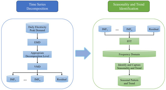
Figure 2.
The process flow chart of data decomposition and seasonality identification.
By applying the variational mode decomposition (VMD) technique, the time series is effectively smoothed through the separation of non-linear and non-stationary components. However, VMD lacks an automated decomposition level adjustment capability. To overcome this limitation, empirical mode decomposition (EMD) is applied as a guide to adjust the decomposition level of VMD, due to its ability to automatically adjust the decomposition level. Following the noise elimination by VMD, the fast Fourier transform (FFT) is utilized to identify and capture any remaining seasonality and trend presented in the denoised data. The seasonality and trend of the daily electricity demand during disrupted situations will be presented as a result.
2.3.1. Data Decomposition
Variational mode decomposition (VMD), introduced in 2014 by Dragomiretskiy and Zosso, is a self-adaptive signal processing method utilized for effectively eliminating noise from the initial time series data. Its primary objective is to partition non-linear and non-stationary data into intrinsic mode functions (IMFs) and residuals. Unlike the conventional empirical mode decomposition (EMD) technique, VMD effectively addresses the mode mixing issue and improves reliability through the application of the alternating direction method of multipliers [76].
Selecting the appropriate decomposition levels for VMD is a significant challenge that many researchers aim to resolve. Excessive decomposition levels can lead to mode aliasing issues and introduce additional noise, while an inadequate number of IMFs can result in insufficient decomposition of the original data [77]. To avoid trial and error and reduce the time consumed in the optimization process, an automatic process is needed. With EMD’s advantageous concept of auto-adjusted decomposition levels, EMD can be applied as a guide for adjusting an appropriate decomposition level in VMD [53].
2.3.2. Seasonality and Trend Identification
Fast Fourier transform (FFT) is a mathematical operation that is widely applied to transform time series data from the time domain to the frequency domain and reveal distinct individual frequencies and dominant frequency components [78]. When dealing with cases where time series data contains hidden seasonality, FFT shows its effectiveness in identifying and capturing underlying seasonal patterns [53].
Electricity demand during the disrupted situation represents a complex time series that contains hidden seasonality. To enhance the forecasting performance of the disrupted situation, it is advantageous to train the forecasting model using the transformed time series data that clearly represent seasonality and trend rather than the original form. In this study, FFT is applied to identify and capture the hidden seasonality and trends that occur in the electricity demand during disrupted situations. The output from the decomposition process is used to train the forecasting model, providing additional data representing the medium-term electricity demand pattern.
2.4. Prediction and Optimization
2.4.1. Data Separation
In classical machine learning approaches, a dataset is typically divided into three subsets: training, validation, and testing datasets [79,80]. Throughout the training process, both the training set error and the validation set error tend to decrease, indicating that the model is learning and improving its performance. However, it is important to be cautious of overfitting, which occurs when the model becomes too specialized to the training set and fails to generalize well to new data. Overfitting is often indicated by a rise in the validation set error, despite a decrease in the training set error. To ensure the best performance, the training parameters (e.g., weights and biases) are retrained under a specific hyperparameter setting until the minimum validation set error is obtained. The optimized training parameters and hyperparameter setting capture the optimal trade-off between fitting the training set and generalizing it to the validation set, which serves as pseudo-unseen data.
The purpose of the testing set is to evaluate the final trained and validated model; however, the test set error is not used during the training process, as it serves as an unbiased measure of the model’s performance on unseen data. The test set error is essentially used for comparing the test set errors of different models and helping researchers make decisions when addressing the task for each model [81].
In the condition of limited data availability during disrupted situations, an excessive proportion of training and validation data makes the model impractical for real application. In this work, the training set contains variables obtained from the daily electricity demand recorded in the 31-day period preceding the target forecast date. In light of the rapid change of electricity demand patterns resulting from emergency and government policies during disrupted situations, this training set enhances the adaptability of the forecasting model by allowing the model to learn the unique characteristics of current electricity demand presented in the historical data. To evaluate the performance of the forecasting model, a separate validation dataset is created using the data from the 7 days before the forecasting target date. Due to daily forecasting, historical days that share the same day type as the target date have a significant effect on the forecasting performance. Considering this perspective, this validation dataset is effectively used for an estimate of how well the model generalizes to the dataset and provides insights into its overall accuracy and reliability.
2.4.2. One-Day-Ahead Forecasting with Rolling Datasets
The disrupted situation introduces unique dynamics to daily electricity demand patterns, leading to continuous changes. To adapt to these patterns, a one-day-ahead forecasting approach [39] is applied for each target date in the testing dataset, as shown in Figure 3. Within this approach, forecasted target dates t, t + 1, and t + 2 are represented by blue, green, and yellow boxes, respectively. Each dotted box delineates the historical training set range for every forecasted target date, containing historical data up to the current or present dataset.
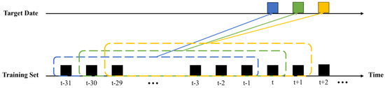
Figure 3.
One-day-ahead forecasting approach.
In disrupted situations with limited input data, traditional dataset splitting methods may reduce data for training. Walk-forward testing [80] is used to maximize data utilization. It involves overlapping splits of the dataset into training, validation, and testing sets, rolling them forward through the time series (Figure 4). This approach efficiently adapts to changing patterns and trends.
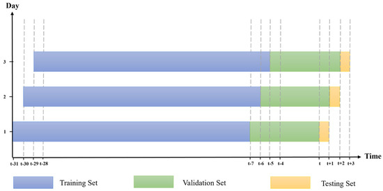
Figure 4.
Rolling dataset using the walk-forward testing approach.
2.4.3. Artificial Neural Network with Grid Search Optimization
Artificial neural network (ANN) is a powerful mathematical technique widely employed in various fields, inspired by the structure of real brains [82]. ANN provides a significant advantage through its ability to learn and uncover relationships between input and output variables [83].
It can adapt and adjust its internal parameters (e.g., weights and biases), allowing it to capture complex patterns and non-linear dependencies in the data. By analyzing and identifying the variables that hold significant influence on the output, ANN can effectively focus on the most relevant information while disregarding less impactful data [84].
One of the most popular ANN structures is the multi-layer feedforward neural network (MLFN). The MLFN structure includes three fundamental layers: the input layer, one or more hidden layers, and the output layer. In the input layer, the values of neurons representing the input variables () are multiplied by adjustable weights (). The resulting weighted inputs are then sent through a non-linear transfer function () within the hidden layer and summation with bias (b) to compute output. This process is repeated for each hidden layer, with the computed output from the previous hidden layer being sent to the next hidden layer or the output layer. A summarized mathematical equation representing the MLFN with a single hidden layer is provided below:
where represents an output from output node; and refer to the transfer functions of the output node and hidden node , respectively; the variable h denotes the number of hidden nodes; variable d refers to the number of input nodes; represents the input data of input node i; b represents bias assigned to neurons; and and denote adjusted weights sent from input node i to hidden node j and hidden node j to the output node, respectively.
2.4.4. Long Short-Term Memory
Long short-term memory (LSTM) is a popular time series forecasting model that is widely employed in various fields. It was proposed by Hochreiter et al. [85] with the aim of operating over the non-linear time-varying problem and making it particularly adept for learning long-term dependencies. LSTM can be seen as an extension of the recurrent neural network (RNN) architecture, integrating essential components called input gate, output gate, and forgetting gate into the RNN neurons [86]. The memory cell is a memory of the network that functions as an accumulation of state information, while the forget gate () decides what information to dispose of from the cell state. A mathematical equation representing a sigmoid function of the forget gate is as follows:
The input gate determines which value from the input should be used to update the cell state by a sigmoid layer referred to as the input gate layer (). Then, the cell state () is updated by a new candidate value vector (). The old cell state () is multiplied with for disposing of the old information and adding the new information by adding term . The mathematical equation of the input gate and the cell state are as follows:
The output gate decides the output based on the cell state. A sigmoid layer of the output gate is applied to filter the cell state, subsequently computing the pertinent information through the multiplication of the cell state with the output value (). The mathematical equations of the output processes are as follows:
where is the input at time , is the output of the model, are defined as weight matrices, and the parameters are represented vectors of bias.
2.4.5. Grid Search Optimization
Grid search (GS) is a systematic process used to test all candidate hyperparameter combinations on grids and select the set of hyperparameters that yields the lowest validation error. Once the better value is identified, finer grid searches are conducted in that specific region. By systematically examining various combinations, grid search helps identify the optimal set of hyperparameter values for a given problem [87]. Due to the straightforward and fundamental approach of GS, this work uses GS as hyperparameter optimization for tuning the hyperparameters of the ANN and LSTM.
3. Case Study: Electricity Peak Demand in Thailand during the COVID-19 Pandemic
3.1. Data Collection and Description
In this paper, the daily electricity peak demand of Thailand during the COVID-19 pandemic is used as a case study for evaluating the efficiency of the proposed model during a disrupted situation. Daily electricity peak demand in megawatts (MW) from January 2018 to December 2020 is used as raw input data. One year of data before the pandemic is included to be able to evaluate the impact. The characteristic of daily electricity peak demand is shown in Figure 5. During the year of the pandemic (2020), the electricity peak demand fluctuated and did not follow the trend of the pre-pandemic years (2018 and 2019). For example, in April 2020, the electricity peak demand dropped compared to the pre-pandemic years. Moreover, the trend of electricity used at the end of April is usually the highest of the year, due to the resuming of many business activities after the Songkran festival. However, in the year of pandemic, the electricity used in April was not much lower. These changes can be attributed to several factors influenced by the restrictions and measures implemented to control the spread of the virus. The autocorrelation function graph (Figure 6) reveals the complex correlation appearing in the electricity peak demand. Due to the non-linear correlation, classical forecasting techniques cannot capture non-linear relationships that appear in time series data during disrupted situations; hence, the utilization of an advanced model becomes imperative to efficiently capture these non-linear relationships.

Figure 5.
Daily electricity peak demand between 2018 and 2020.
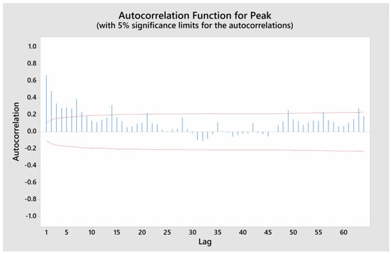
Figure 6.
Autocorrelation function graph of electricity peak demand during the COVID-19 pandemic.
As this case study considers the impact of the COVID-19 pandemic, the data involving COVID-19 factors and level of lockdown are collected. The level of lockdown is treated as a government intervention policy. The level is announced by the government of Thailand ranking from zero (no-lockdown stage) to six (declaration of a state/national emergency stage). The higher the level, the stricter the lockdown. The description and timeline of the lockdown stages in Thailand are shown in Table 5. The data regarding six COVID-19 factors, including the number of daily infections, daily deaths, daily recoveries, current COVID-19 in-patients, cumulative vaccinations, and cumulative full vaccinations are provided by the Thai Ministry of Public Health. The COVID-19 factors and level of lockdown are ranged daily from January to December 2020, as shown in Figure 7. The statistical description of daily electricity peak demand and the six factors are presented in Table 6.
Table 5.
Timeline and description of the COVID-19 lockdown.
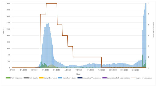
Figure 7.
Dataset of six COVID-19 factors and level of lockdown.
Table 6.
The statistical description of daily electricity peak demand and the COVID-19 factors.
3.2. Data Separation and Sensitivity Factors Identification
Following the identification of whether the target period falls under the government intervention policy, the total daily electricity peak demand from 2018 to 2020 is divided into three input sets: short-term, medium-term, and long-term. The short-term input set contains the most recent historical data leading up to the target forecast date in 2020. The medium-term input set consists of data from the week and month immediately prior to the target date. In contrast, the long-term input set includes the data from the previous year (2019), covering the target date and the data from one week before the target day in the previous year.
In disrupted situations, sensitivity factors play an important role in understanding the pandemic situation, which reflects the pattern of daily electricity demand. This understanding is essential for adapting to changes in electricity demand patterns during the pandemic. In this work, the sensitivity factors are set based on sensitivity level. Only the sensitivity factors provided by the government sector that affect sensitivity level are selected to train the forecasting model. In the case of the COVID-19 pandemic, the level of lockdown and the six COVID-19 factors are used as sensitivity factors.
3.3. Case 1: Interference with Government Policy
In case the targeted period is influenced by government intervention policies, the short-term input set is separated into training, validation, and testing sets using the data separation theory explained in Section 2.4.1. The training set and validation set are utilized for developing and refining the LSTM model, respectively. Particularly, the LSTM’s hyperparameters are fine-tuned using grid search (GS). In this work, the LSTM-based GS optimization is executed through MATLAB R2022b software. GS is performed on three key hyperparameters: the number of hidden nodes, training cycles, and learning rate, each represented as an array of values. The GS method trains LSTM with all possible combinations of hyperparameter values within the defined range denoted as a grid (see Table 7).
Table 7.
Defined ranges of LSTM hyperparameters.
To perform one-day-ahead forecasting with rolling dataset, when the target date moves to the new date, input data are updated and a new GS optimization is performed again. Thus, the optimal hyperparameter set is varied, depending on the target date. After searching through all hyperparameter combinations, the best-found LSTM model is selected, and the model performance is evaluated with the test set.
3.4. Case 2: Noninterference with Government Policy
3.4.1. Input Variable Filtering for the Case of the COVID-19 Pandemic
Important input variables included in the forecasting model are selected by the stepwise regression method. In this work, Minitab R2022b software is used for performing this process. The input dataset for computing stepwise regression contains 24 months of raw data preceding the month of the target date. For example, if the target date is 1 January 2020, the electricity peak demand considered spans from 1 January 2018 to 31 December 2019. However, when the target date moves to a new month, the input dataset is updated, and a new stepwise regression is refit. The total number of candidate input variables used in stepwise regression is 24, as shown in Table 8. The list of significant input variables changes every month due to the refitting of the stepwise regression process. Stepwise regression is applied to the medium-term input set for selecting the significant medium-term input variables, which are then used as input variables in the forecasting model.
Table 8.
The candidate input variables used in stepwise regression.
The SD method is used to select the date from the long-term input set that is similar to the target date by considering the day type criterion. An example of the steps to perform SD for the disrupted situation is presented in Section 2.2.4. The output from the SD is the date that is most similar to the target date. The variables of a similar date, including electricity peak demand, day of the week index, special holiday index, historical electricity peak demand, LMA, and MA(P) are screened by stepwise regression for later use as long-term input variables in the forecasting model.
3.4.2. Data Decomposition
Referring to Figure 5, the original daily electricity peak demand of 1096 observations from 2018 to 2020 shows a complex pattern due to non-linear and non-stationary components, especially during the periods of the COVID-19 pandemic. To handle the complex pattern during the pandemic, VMD is applied to the medium-term input set in the year 2020. VMD decomposes the original time series into k intrinsic mode functions (IMFs). The value of k represents the decomposition level of VMD, which is determined based on guidance from EMD. According to the pattern of dataset used in this case study, the output of decomposition level (k) suggested by EMD is equal to five. The other parameters are set based on the default values of the MATLAB software. The maximum number of optimization iterations is set to 500, the penalty level is set to 1000, and peaks are utilized as the method for initializing the central frequencies.
After using VMD to uncover the underlying structures and extract meaningful information from the complex pattern, FFT is applied to all IMFs and residuals for identifying and capturing the hidden seasonality and trend of the COVID-19 pandemic that remain in the medium-term input set. Applying FFT to these components reveals clearer identification and easier capture of the resulting seasonality and trend components, as shown in Figure 8.
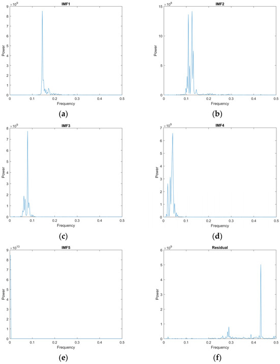
Figure 8.
Seasonality and trend identification after applying FFT to all IMFs and residuals. (a) IMF1; (b) IMF2; (c) IMF3; (d) IMF4; (e) IMF5; (f) residual.
3.4.3. Data Splitting and ANN-Based Grid Search Optimization
The processed dataset consists of output from VMD-EMD-FFT, stepwise regression, and SD is separated into training set, validation set, and test set, following the data separation theory described in Section 2.4.1. The training set and validation set are used to build and tune the ANN, respectively. Specifically, grid search (GS) is used for ANN’s hyperparameter tuning. In this work, ANN-based GS optimization is conducted by RapidMiner Studio 9.1 software. GS is performed on three hyperparameters, consisting of the number of hidden nodes, training cycles, and learning rate. Each value of hyperparameters is represented as an array. The GS method trains ANN with all possible combinations of hyperparameter values within the defined range denoted as a grid (see Table 9).
Table 9.
Defined ranges of ANN hyperparameters.
One-day-ahead forecasting with a rolling dataset is conducted using the same procedures outlined, as described in Section 3.3. After searching through all hyperparameter combinations, the best-found ANN model is chosen, and the model performance is evaluated with the test set.
3.5. Performance Measurement
The model performance is evaluated by using three measurements, which are mean absolute error (MAE), mean absolute percentage error (MAPE), and root mean square error (RMSE). MAE measures the magnitude of errors without considering their direction. MAPE expresses the absolute value of errors as a percentage of the actual values, which makes it useful for comparing across different models. RMSE provides a measure of the average magnitude of the errors by calculating the square root of the average squared differences between the forecasted values and the actual values. RMSE is sensitive to large errors due to the summation of squared differences in the formula. In contrast to RMSE, MAE and MAPE consider absolute or relative differences which make them less sensitive to outliers. The formula of MAE, MAPE, and RMSE are shown in Equation (11), Equation (12), and Equation (13), respectively.
where represents an actual value of electricity peak demand in period i; represents the forecast electricity peak demand in period i; and n represents the total number of forecasting periods.
3.6. Experimental Results and Discussion
A 1-year experiment containing 12 months from January 2020 to December 2020 is conducted to test the performance of the models for handling the disrupted situation. The assumption of the proposed model is verified by applying three benchmark models to the 1-year dataset. The first model is implemented by applying an ANN-based GS optimization to the preprocessed data obtained from stepwise regression, SD with the Euclidean distance criterion, and the decomposition and seasonality-capturing method proposed by Aswanuwath et al. [53]. The second model utilizes an ANN-based GS optimization with a significant long-term input set chosen from SD with a day type criterion. Additionally, the second model integrates a key medium-term input set selected from stepwise regression, along with processed data from VMD-EMD-FFT. The third model is conducted by applying LSTM-based GS optimization with a short-term input set. One-year comparison results between the three benchmark models for testing performance are shown in Table 10.
Table 10.
Monthly results in 1 year representing testing performance.
Referring to the results in Table 10, benchmark model 1 performs worse than benchmark models 2 and 3. This discrepancy can be attributed to the SD based on the Euclidean distance criterion. The SD used in benchmark model 1 primarily emphasizes the similarity between the demand of the target date and the candidate date in the pre-pandemic year. Consequently, the model struggles to efficiently handle demand in pandemic situations as it heavily relies on data from the pre-pandemic year. In contrast, benchmark model 2 uses SD based on day type criterion, training the model with different datasets that contain medium-term and long-term characteristics of time periods. It provides good performance in situations where the target period is not influenced by government intervention policies (level of lockdown equal to 0). Its effectiveness stems from the demand characteristic during this situation, sharing similarities with the pre-pandemic year due to the resumption of economic activities and tourism. However, its performance decreases when faced with dramatic changes in demand and unique patterns caused by government policy intervention, as it excessively depends on medium-term and long-term data. When dealing with the dramatic changes caused by government policies (level of lockdown equal to 1–6), LSTM demonstrates the highest performance due to its adeptness in handling short-term data, allowing for swift adaptation to immediate shifts. LSTM excels in extracting patterns and dependencies from short-term data, allowing it to capture rapid fluctuations and evolving trends with precision. This capacity enables LSTM to respond effectively to dynamic scenarios, making it highly adept at forecasting unpredictable changes caused by government interventions.
These insights provide an understanding of each model’s performance, offering valuable guidance for decision making in diverse situations. Under normal situations, benchmark model 1 stands as a suitable choice for forecasting electricity demand. In disrupted scenarios where there is no government intervention, benchmark model 2 demonstrates its suitability for accurate electricity demand forecasting. However, in situations disrupted by government policies, benchmark model 3 stands out as the appropriate model for accurately forecasting electricity demand. After applying these insights to the whole year of the COVID-19 pandemic, the results demonstrate that the proposed hybrid model surpasses the individual benchmark models (benchmark models 1, 2, and 3), as shown at the bottom of Table 10.
During the pandemic year, the challenge of electricity demand forecasting arose not only due to government interventions, but also occurred throughout the entirety of the pandemic year. The most challenging situation occurred during the pandemic period that was not influenced by government intervention policies (level of lockdown equal to 0). In this period, electricity demand contained a mixed pattern between the pre-pandemic year and the pandemic period intervened by government policy (level of lockdown equal to 1–6). Despite the absence of strict government interventions, people remained cautious of the ongoing pandemic and continued to work remotely and minimize economic activities, resulting in a unique demand pattern that reflected a blend of pre-existing and pandemic-influenced behaviors.
When considering the forecasting error, Figure 9 shows the daily errors of the proposed model. High forecasting errors occur during mid-April, mid-November, and December. These peaks coincide with specific events and policy shifts, providing crucial insights into the nature of these errors. During the period of lockdown, the largest error presents at the highest level of lockdown. The error gradually declines as the level of lockdown remains constant and increases when the level changes, as shown in Figure 10. However, an abnormal pattern appeared at the end of July due to the unexpected governmental declaration of additional holidays, causing disruption in the error pattern. Contrary to the previous tendency, a large error occurred later in the year, reaching a peak in mid-November due to the extension of the national emergency declaration. Towards late December, an error arose again due to a huge cluster of coronavirus cases, marking the highest recorded daily infection rate in Thailand. Despite the absence of a lockdown during this period, people continued to reduce social interactions, activities, and tourism due to the rising number of daily infections. This situation significantly changed the electricity demand pattern by the end of the year, marking a characteristic of demand totally different from the pre-pandemic year, leading to a large error.
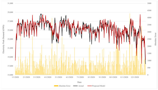
Figure 9.
The daily forecasting error of the proposed model on the test dataset.
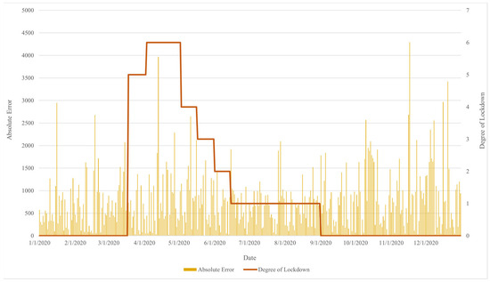
Figure 10.
The forecasting error related to the level of lockdown.
The comparative performance between the proposed model and prior studies is shown in Table 11. This comparative analysis is conducted with the other models that appear in the literature such as benchmark model 1 [53], LSTM [88], XGBoost [89], and SVM [90]. All comparative models follow the same structure, as outlined in prior research. According to the result shown in Table 11, the proposed model not only surpasses all benchmark models but also outperforms all other comparative models in all three measures (i.e., MAPE, RMSE, and MAE).
Table 11.
Performance comparison between the proposed model and the previous studies applied with testing dataset.
Based on the results, the proposed model performance on the test set confirms the superiority of handling the whole year of disrupted situations (with and without government intervention policies). With the appropriate forecasting model containing various characteristics across time periods and suited to the specific situation, the increase in flexibility and adaptability for capturing unnoticeable changes in electricity demand during the year of the pandemic is evident. The proposed model not only shows a significant improvement, but also reduces the number of input variables. The reduction is achieved by training the model solely with important variables and variables indicating the date that closely resembles the target forecast date. Furthermore, the GS optimization technique is applied to the proposed model for the best possible outcomes, while avoiding using forecasted input variables for ensuring the reliability and accuracy of the results. Overall, the proposed model delivers more accurate and unbiased forecasting results, making it a promising and effective approach for future disrupted situations.
4. Conclusions
Disrupted situations have brought significant changes in the energy sector of many countries. Understanding the shifts in electricity demand, and their implications on electricity demand forecasting, becomes crucial to ensure the reliable operation of the electricity grid. With the aim of mitigating the impact of future disruptions on electricity demand forecasting, this work proposed a hybrid approach for handling hybrid scenarios (with and without government intervention). The core strength of this approach lies in its capacity to identify and utilize forecasting techniques that correspond to specific scenarios, integrating methods such as stepwise regression, SD-based day type criterion, VMD-EMD-FFT, ANN-based GS, and LSTM-based GS. Electricity peak demand data in Thailand during the year of the COVID-19 situation are used as a case study. This work introduces a new criterion to separate short-term, medium-term, and long-term input sets for the context of disrupted situations, along with the new criterion of SD for handling a situation where the demand of a candidate date shows low similarity to the target date. To enhance the model’s flexibility and adaptability for daily change, one-day-ahead forecasting with rolling datasets and pandemic sensitivity factors is applied. Additionally, the insights gleaned from model performances offer valuable guidance for decision making across diverse situations. As demonstrated in Table 10, benchmark model 1 proves effective in normal scenarios, while in disrupted scenarios lacking government intervention, benchmark model 2 serves as a suitable choice. In situations disrupted by government policies, benchmark model 3 emerges as the appropriate choice for accurate electricity demand forecasting.
This study aligns with multiple Sustainable Development Goals (SDGs), including Quality Education (SDG 4), Decent Work and Economic Growth (SDG 8), Industry, Innovation, and Infrastructure (SDG 9), Responsible Consumption and Production (SDG 12), and Climate Action (SDG 13), by disseminating electricity forecasting insights and offering valuable guidance for decision making in diverse situations. This approach aids in accurate forecasting, enabling efficient resource allocation, minimizing energy production wastage, mitigating environmental impact, reducing financial losses, and fostering sustainable economic growth.
The proposed approach successfully improved flexibility and gave superior performance over the comparative models in terms of MAPE, RMSE, and MAE. Moreover, the proposed approach requires a relatively short computational time and avoids using input variables that require prior forecasts. Thus, with high flexibility, reduced number of input variables, and less computational time, the proposed approach is suitable for daily electricity peak demand forecasting under disrupted situations. Although the proposed approach can give high forecasting accuracy and stability, it carries certain limitations that suggest avenues for further exploration. One potential area for improvement involves testing the approach using advanced machine learning techniques beyond the utilization of ANN and LSTM, thereby broadening the scope of model sophistication. Additionally, renewable energy has seen significant growth and transformation worldwide to support economic development and environmental protection. However, this study’s focus on renewable energy remains relatively limited within the proposed forecasting framework, indicating a potential avenue for future research exploration.
Author Contributions
Conceptualization, L.A., W.P., J.B., J.K. and V.-N.H.; Data curation, L.A., W.P. and J.B.; Formal analysis, L.A., W.P. and J.B.; Investigation, L.A., W.P., J.B., J.K. and V.-N.H.; Methodology, L.A., W.P., J.B., J.K. and V.-N.H.; Software, L.A. and W.P.; Supervision, W.P., J.B., J.K. and V.-N.H.; Validation, L.A., W.P., J.B., J.K. and V.-N.H.; Writing—original draft, L.A. and W.P.; Writing—review and editing, W.P., J.B., J.K. and V.-N.H. All authors have read and agreed to the published version of the manuscript.
Funding
This study was supported by Thammasat University Research Fund, Contract No. TUFT35/2564.
Data Availability Statement
The data are not publicly available due to project privacy issues.
Acknowledgments
The authors would like to express our gratitude to the Electricity Generating Authority of Thailand (EGAT) for providing the data used in this research and the Center of Excellence in Logistics and Supply Chain Systems Engineering and Technology (LogEn), Sirindhorn International Institute of Technology (SIIT), Thammasat University, for their support in carrying out this research. The first author acknowledges the dual doctoral degree scholarship awarded by Sirindhorn International Institute of Technology (SIIT) Thammasat University, National Science and Technology Development Agency (NSTDA), and Japan Advanced Institute of Science and Technology (JAIST).
Conflicts of Interest
The authors declare no conflicts of interest.
References
- Islam, S.M. Principles of electricity demand forecasting. Power Eng. J. 1997, 10, 139–143. [Google Scholar]
- Xing, X.; Yan, Y.; Zhang, H.; Long, Y.; Wang, Y.; Liang, Y. Optimal design of distributed energy systems for industrial parks under gas shortage based on augmented ε-constraint method. J. Clean. Prod. 2019, 218, 782–795. [Google Scholar] [CrossRef]
- Dong, L.; Lao, L.; Yang, Y.; Luo, J. Probabilistic Load Flow Analysis Considering Power System Random Factors and Their Relevance. In Proceedings of the Asia-Pacific Power and Energy Engineering Conference, Wuhan, China, 15–18 March 2011. [Google Scholar]
- Ranaweera, D.K.; Karady, G.G.; Farmer, R.G. Economic Impact Analysis of Load Forecasting. IEEE Trans. Power Syst. 1997, 12, 1388–1392. [Google Scholar] [CrossRef]
- Luo, X.; Wang, J.; Dooner, M.; Clarke, J. Overview of current development in electrical energy storage technologies and the application potential in power system operation. Appl. Energy 2015, 137, 511–536. [Google Scholar] [CrossRef]
- Zhang, H.; Song, X.; Xia, T.; Yuan, M.; Fan, Z.; Shibasaki, R.; Liang, Y. Battery electric vehicles in Japan: Human mobile behavior based adoption potential analysis and policy target response. Appl. Energy 2018, 220, 527–535. [Google Scholar] [CrossRef]
- Ramzan, M.; Razi, U.; Quddoos, M.U.; Adebayo, T.S. Do green innovation and financial globalization contribute to the ecological sustainability and energy transition in the United Kingdom? Policy insights from a bootstrap rolling window approach. Sustain. Dev. 2023, 31, 393–414. [Google Scholar] [CrossRef]
- Huterski, R.; Huterska, A.; Zdunek-Rosa, E.; Voss, G. Evaluation of the Level of Electricity Generation from Renewable Energy Sources in European Union Countries. Energies 2021, 14, 8150. [Google Scholar] [CrossRef]
- Piekut, M. The Consumption of Renewable Energy Sources (Res) by the European Union Households between 2004 and 2019. Energies 2021, 14, 5560. [Google Scholar] [CrossRef]
- Igliński, B.; Kiełkowska, U.; Pietrzak, M.B.; Skrzatek, M.; Kumar, G.; Piechota, G. The regional energy transformation in the context of renewable energy sources potential. Renew. Energy 2023, 218, 119246. [Google Scholar] [CrossRef]
- Balcerzak, A.P.; Uddin, G.S.; Igliński, B.; Pietrzak, M.B. Global energy transition: From the main determinants to economic challenges. Equilibrium. Q. J. Econ. Econ. Policy 2023, 18, 597–608. [Google Scholar] [CrossRef]
- Skvarciany, V.; Lapinskaite, I.; Volskyte, G. Circular economy as assistance for sustainable development in OECD countries. Oeconomia Copernicana 2021, 12, 11–34. [Google Scholar] [CrossRef]
- Narajewski, M.; Ziel, F. Change in Electricity Demand Pattern in Europe Due to COVID-19 Shutdowns. arXiv 2020, arXiv:2004.14864. [Google Scholar]
- Chen, Y.; Yang, W.; Zhang, B. Using Mobility for Electrical Load Forecasting During the COVID-19 Pandemic. arXiv 2020, arXiv:2006.08826. [Google Scholar]
- Baek, S.; Mohanty, S.K.; Glambosky, M. COVID-19 and stock market volatility: An industry level analysis. Financ. Res. Lett. 2020, 37, 101748. [Google Scholar] [CrossRef] [PubMed]
- Vitenu-Sackey, P.A.; Barfi, R. The Impact of Covid-19 Pandemic on the Global Economy: Emphasis on Poverty Alleviation and Economic Growth. Econ. Financ. Lett. 2021, 8, 32–43. [Google Scholar] [CrossRef]
- Klemeš, J.J.; Van Fan, Y.; Jiang, P. The energy and environmental footprints of COVID-19 fighting measures—PPE, disinfection, supply chains. Energy 2020, 211, 118701. [Google Scholar] [CrossRef]
- Aktar, M.A.; Alam, M.M.; Al-Amin, A.Q. Global economic crisis, energy use, CO2 emissions, and policy roadmap amid COVID-19. Sustain. Prod. Consum. 2021, 26, 770–781. [Google Scholar] [CrossRef]
- Cheshmehzangi, A. COVID-19 and household energy implications: What are the main impacts on energy use? Heliyon 2020, 6, E05202. [Google Scholar] [CrossRef]
- Abulibdeh, A.; Zaidan, E.; Jabbar, R. The impact of COVID-19 pandemic on electricity consumption and electricity demand forecasting accuracy: Empirical evidence from the state of Qatar. Energy Strateg. Rev. 2022, 44, 100980. [Google Scholar] [CrossRef]
- Yukseltan, E.; Yucekaya, A.; Bilge, A.H. Forecasting electricity demand for Turkey: Modeling periodic variations and demand segregation. Appl. Energy 2017, 193, 287–296. [Google Scholar] [CrossRef]
- Son, H.; Kim, C. Short-term forecasting of electricity demand for the residential sector using weather and social variables. Resour. Conserv. Recycl. 2017, 123, 200–207. [Google Scholar] [CrossRef]
- Pappas, S.S.; Ekonomou, L.; Karamousantas, D.C.; Chatzarakis, G.E.; Katsikas, S.K.; Liatsis, P. Electricity demand loads modeling using AutoRegressive Moving Average (ARMA) models. Energy 2008, 33, 1353–1360. [Google Scholar] [CrossRef]
- Newsham, G.R.; Birt, B.J. Building-Level Occupancy Data to Improve ARIMA-Based Electricity Use Forecasts. In Proceedings of the 2nd ACM Workshop on Embedded Sensing Systems for Energy-Efficiency in Building, Zurich, Switzerland, 2 November 2010. [Google Scholar]
- Hamzacebi, C.; Es, H.A. Forecasting the annual electricity consumption of Turkey using an optimized grey model. Energy 2014, 70, 165–171. [Google Scholar] [CrossRef]
- Alasali, F.; Nusair, K.; Alhmoud, L.; Zarour, E. Impact of the COVID-19 Pandemic on Electricity Demand and Load Forecasting. Sustainability 2021, 13, 1435. [Google Scholar] [CrossRef]
- Huang, L.; Liao, Q.; Qiu, R.; Liang, Y.; Long, Y. Prediction-based analysis on power consumption gap under long-term emergency: A case in China under COVID-19. Appl. Energy 2021, 283, 116339. [Google Scholar] [CrossRef] [PubMed]
- Obst, D.; de Vilmarest, J.; Goude, Y. Adaptive Methods for Short-Term Electricity Load Forecasting during COVID-19 Lockdown in France. IEEE Trans. Power Syst. 2021, 36, 4754–4763. [Google Scholar] [CrossRef] [PubMed]
- Şahin, U.; Ballı, S.; Chen, Y. Forecasting seasonal electricity generation in European countries under Covid-19-induced lockdown using fractional grey prediction models and machine learning methods. Appl. Energy 2021, 302, 117540. [Google Scholar] [CrossRef] [PubMed]
- Hippert, H.S.; Pedreira, C.E.; Souza, R.C. Neural Networks for Short-Term Load Forecasting: A Review and Evaluation. IEEE Trans. Power Syst. 2001, 16, 44–55. [Google Scholar] [CrossRef]
- L’Heureux, A.; Grolinger, K.; Elyamany, H.F.; Capretz, M.A.M. Machine Learning with Big Data: Challenges and Approaches. IEEE Access 2017, 5, 7776–7797. [Google Scholar] [CrossRef]
- Chen, B.J.; Chang, M.W.; Lin, C.J. Load Forecasting Using Support Vector Machines: A Study on EUNITE Competition 2001. IEEE Trans. Power Syst. 2004, 19, 1821–1830. [Google Scholar] [CrossRef]
- Ekonomou, L. Greek long-term energy consumption prediction using artificial neural networks. Energy 2010, 35, 512–517. [Google Scholar] [CrossRef]
- Bouktif, S.; Fiaz, A.; Ouni, A.; Serhani, M.A. Optimal Deep Learning LSTM Model for Electric Load Forecasting using Feature Selection and Genetic Algorithm: Comparison with Machine Learning Approaches. Energies 2018, 11, 1636. [Google Scholar] [CrossRef]
- Burnaev, E.V.; Panov, M.E.; Zaytsev, A.A. Regression on the Basis of Nonstationary Gaussian Processes with Bayesian Regularization. J. Commun. Technol. Electron. 2016, 61, 661–671. [Google Scholar] [CrossRef]
- Sözen, A.; İzgeç, M.M.; Kırbaş, İ.; Kazancıoğlu, F.Ş.; Tuncer, A.D. Overview, modeling and forecasting the effects of COVID-19 pandemic on energy market and electricity demand: A case study on Turkey. Energy Sources Part A Recover. Util. Environ. Eff. 2021, 1–16. [Google Scholar] [CrossRef]
- Li, X.; Wang, Y.; Ma, G.; Chen, X.; Shen, Q.; Yang, B. Electric load forecasting based on Long-Short-Term-Memory network via simplex optimizer during COVID-19. Energy Rep. 2022, 8, 1–12. [Google Scholar] [CrossRef]
- Liu, X.; Lin, Z. Impact of COVID-19 pandemic on electricity demand in the UK based on multivariate time series forecasting with Bidirectional Long Short Term Memory. Energy 2021, 227, 120455. [Google Scholar] [CrossRef] [PubMed]
- Lu, H.; Ma, X.; Ma, M. A hybrid multi-objective optimizer-based model for daily electricity demand prediction considering COVID-19. Energy 2021, 219, 119568. [Google Scholar] [CrossRef]
- Hu, C.; Zhang, J.; Yuan, H.; Gao, T.; Jiang, H.; Yan, J.; Wenzhong Gao, D.; Wang, F.Y. Black swan event small-sample transfer learning (BEST-L) and its case study on electrical power prediction in COVID-19. Appl. Energy 2022, 309, 118458. [Google Scholar] [CrossRef]
- Wang, D.; Luo, H.; Grunder, O.; Lin, Y.; Guo, H. Multi-step ahead electricity price forecasting using a hybrid model based on two-layer decomposition technique and BP neural network optimized by firefly algorithm. Appl. Energy 2017, 190, 390–407. [Google Scholar] [CrossRef]
- AL-Musaylh, M.S.; Deo, R.C.; Li, Y.; Adamowski, J.F. Two-phase particle swarm optimized-support vector regression hybrid model integrated with improved empirical mode decomposition with adaptive noise for multiple-horizon electricity demand forecasting. Appl. Energy 2018, 217, 422–439. [Google Scholar] [CrossRef]
- Wang, G.; Wang, X.; Wang, Z.; Ma, C.; Song, Z. A VMD-CISSA-LSSVM Based Electricity Load Forecasting Model. Mathematics 2022, 10, 28. [Google Scholar] [CrossRef]
- Yu, Y.; Li, W.; Sheng, D.; Chen, J. A novel sensor fault diagnosis method based on Modified Ensemble Empirical Mode Decomposition and Probabilistic Neural Network. Measurement 2015, 68, 328–336. [Google Scholar] [CrossRef]
- Torres, M.E.; Colominas, M.A.; Schlotthauer, G.; Flandrin, P. A Complete Ensemble Empirical Mode Decomposition with Adaptive Noise. In Proceedings of the 2011 IEEE international conference on acoustics, speech and signal processing (ICASSP), Prague, Czech Republic, 22–27 May 2011. [Google Scholar]
- Xiao, Q.; Li, J.; Sun, J.; Feng, H.; Jin, S. Natural-gas pipeline leak location using variational mode decomposition analysis and cross-time–frequency spectrum. Measurement 2018, 124, 163–172. [Google Scholar] [CrossRef]
- Jiang, P.; Li, R.; Liu, N.; Gao, Y. A novel composite electricity demand forecasting framework by data processing and optimized support vector machine. Appl. Energy 2020, 260, 114243. [Google Scholar] [CrossRef]
- Zhou, Y.; Zhu, Z. A hybrid method for noise suppression using variational mode decomposition and singular spectrum analysis. J. Appl. Geophys. 2019, 161, 105–115. [Google Scholar] [CrossRef]
- Zhang, X.; Miao, Q.; Zhang, H.; Wang, L. A parameter-adaptive VMD method based on grasshopper optimization algorithm to analyze vibration signals from rotating machinery. Mech. Syst. Signal Process. 2018, 108, 58–72. [Google Scholar] [CrossRef]
- Ding, J.; Xiao, D.; Li, X. Gear Fault Diagnosis Based on Genetic Mutation Particle Swarm Optimization VMD and Probabilistic Neural Network Algorithm. IEEE Access 2020, 8, 18456–18474. [Google Scholar] [CrossRef]
- Gai, J.; Shen, J.; Hu, Y.; Wang, H. An integrated method based on hybrid grey wolf optimizer improved variational mode decomposition and deep neural network for fault diagnosis of rolling bearing. Measurement 2020, 162, 107901. [Google Scholar] [CrossRef]
- Venter, G. Review of Optimization Techniques. In Encyclopedia of Aerospace Engineering; John Wiley & Sons Ltd.: Chichester, UK, 2010; pp. 1–10. ISBN 9780470686652. [Google Scholar]
- Aswanuwath, L.; Pannakkong, W.; Buddhakulsomsiri, J.; Karnjana, J.; Huynh, V.-N. A Hybrid Model of VMD-EMD-FFT, Similar Days Selection Method, Stepwise Regression, and Artificial Neural Network for Daily Electricity Peak Load Forecasting. Energies 2023, 16, 1860. [Google Scholar] [CrossRef]
- Galelli, S.; Humphrey, G.B.; Maier, H.R.; Castelletti, A.; Dandy, G.C.; Gibbs, M.S. An evaluation framework for input variable selection algorithms for environmental data-driven models. Environ. Model. Softw. 2014, 62, 33–51. [Google Scholar] [CrossRef]
- Taormina, R.; Chau, K.W. Data-driven input variable selection for rainfall-runoff modeling using binary-coded particle swarm optimization and Extreme Learning Machines. J. Hydrol. 2015, 529, 1617–1632. [Google Scholar] [CrossRef]
- Bonnlander, B.V.; Weigend, A.S. Selecting Input Variables Using Mutual Information and Nonparametric Density Estimation. In Proceedings of the International Symposium on Artificial Neural Networks, Tainan, China, 28 June–2 July 1994. [Google Scholar]
- Bowden, G.J.; Maier, H.R.; Dandy, G.C. Input determination for neural network models in water resources applications. Part 2. Case study: Forecasting salinity in a river. J. Hydrol. 2005, 301, 93–107. [Google Scholar] [CrossRef]
- Niu, D.; Wang, Y.; Wu, D.D. Power load forecasting using support vector machine and ant colony optimization. Expert Syst. Appl. 2010, 37, 2531–2539. [Google Scholar] [CrossRef]
- Gabriels, W.; Goethals, P.L.M.; Dedecker, A.P.; Lek, S.; De Pauw, N. Analysis of macrobenthic communities in Flanders, Belgium, using a stepwise input variable selection procedure with artificial neural networks. Aquat. Ecol. 2007, 41, 427–441. [Google Scholar] [CrossRef]
- Mandal, P.; Senjyu, T.; Funabashi, T. Neural networks approach to forecast several hour ahead electricity prices and loads in deregulated market. Energy Convers. Manag. 2006, 47, 2128–2142. [Google Scholar] [CrossRef]
- Chen, Y.; Luh, P.B.; Guan, C.; Zhao, Y.; Michel, L.D.; Coolbeth, M.A.; Friedland, P.B.; Rourke, S.J. Short-Term Load Forecasting: Similar Day-Based Wavelet Neural Networks. IEEE Trans. Power Syst. 2010, 25, 322–330. [Google Scholar] [CrossRef]
- Fallah, S.N.; Ganjkhani, M.; Shamshirband, S.; Chau, K. wing Computational Intelligence on Short-Term Load Forecasting: A Methodological Overview. Energies 2019, 12, 393. [Google Scholar] [CrossRef]
- Mu, Q.; Wu, Y.; Pan, X.; Huang, L.; Li, X. Short-Term Load Forecasting Using Improved Similar Days Method. In Proceedings of the 2010 Asia-Pacific Power and Energy Engineering Conference (APPEEC), Chengdu, China, 28–31 March 2010. [Google Scholar]
- Zheng, H.; Yuan, J.; Chen, L. Short-Term Load Forecasting Using EMD-LSTM Neural Networks with a Xgboost Algorithm for Feature Importance Evaluation. Energies 2017, 10, 1168. [Google Scholar] [CrossRef]
- Park, R.-J.; Song, K.-B.; Kwon, B.-S. Short-Term Load Forecasting Algorithm Using a Similar Day Selection Method Based on Reinforcement Learning. Energies 2020, 13, 2640. [Google Scholar] [CrossRef]
- Senjyu, T.; Takara, H.; Uezato, K.; Funabashi, T. One-Hour-Ahead Load Forecasting Using Neural Network. IEEE Trans. Power Syst. 2002, 17, 113–118. [Google Scholar] [CrossRef]
- The Asia Foundation. Available online: https://asiafoundation.org/where-we-work/thailand/ (accessed on 21 February 2022).
- Giordano, F.; La Rocca, M.; Perna, C. Input Variable Selection in Neural Network Models. Commun. Stat. Theory Methods 2014, 43, 735–750. [Google Scholar] [CrossRef]
- Guyon, I.; Elisseeff, A. An Introduction to Variable and Feature Selection. J. Mach. Learn. Res. 2003, 3, 1157–1182. [Google Scholar]
- Humpage, S. An introduction to regression analysis. Sensors 2000, 17, 68–74. [Google Scholar] [CrossRef]
- Lucà, F.; Buttafuoco, G.; Terranova, O. GIS and Soil. Compr. Geogr. Inf. Syst. 2018, 3, 37–50. [Google Scholar] [CrossRef]
- Yildiz, B.; Bilbao, J.I.; Sproul, A.B. A review and analysis of regression and machine learning models on commercial building electricity load forecasting. Renew. Sustain. Energy Rev. 2017, 73, 1104–1122. [Google Scholar] [CrossRef]
- Johnsson, T. A procedure for stepwise regression analysis. Stat. Pap. 1992, 33, 21–29. [Google Scholar] [CrossRef]
- Chatterjee, S.; Hadi, A.S. Regression Analysis by Example, 5th ed.; John Wiley & Sons Ltd.: Hoboken, NJ, USA, 2012. [Google Scholar]
- Ramón, J.; Espasa, A.; Grafe, R. Forecasting the electricity load from one day to one week ahead for the Spanish system operator. Int. J. Forecast. 2008, 24, 588–602. [Google Scholar] [CrossRef]
- Dragomiretskiy, K.; Zosso, D. Variational Mode Decomposition. IEEE Trans. Signal Process. 2014, 62, 531–544. [Google Scholar] [CrossRef]
- Zhou, F.; Zhou, H.; Li, Z.; Zhao, K. Multi-Step Ahead Short-Term Electricity Load Forecasting Using VMD-TCN and Error Correction Strategy. Energies 2022, 15, 5375. [Google Scholar] [CrossRef]
- Musbah, H. SARIMA Model Forecasting of Short-Term Electrical Load Data Augmented by Fast Fourier Transform Seasonality Detection. In Proceedings of the 2019 IEEE Canadian Conference of Electrical and Computer Engineering (CCECE), Edmonton, AB, Canada, 5–8 May 2019. [Google Scholar]
- Aras, S.; Kocakoç, T.D. A new model selection strategy in time series forecasting with artificial neural networks: IHTS. Neurocomputing 2016, 174, 974–987. [Google Scholar] [CrossRef]
- Kaastraa, I.; Boydb, M. Designing a neural network for forecasting financial time series. Neurocomputing 1996, 10, 215–236. [Google Scholar] [CrossRef]
- Negash, B.M.; Yaw, A.D. Artificial neural network based production forecasting for a hydrocarbon reservoir under water injection. Pet. Explor. Dev. 2020, 47, 383–392. [Google Scholar] [CrossRef]
- Svozil, D.; Kvasnička, V.; Pospíchal, J. Introduction to multi-layer feed-forward neural networks. Chemom. Intell. Lab. Syst. 1997, 39, 43–62. [Google Scholar] [CrossRef]
- Lauret, P.; Fock, E.; Randrianarivony, R.N.; Manicom-Ramsamy, J.F. Bayesian neural network approach to short time load forecasting. Energy Convers. Manag. 2008, 49, 1156–1166. [Google Scholar] [CrossRef]
- Dedinec, A.; Filiposka, S.; Dedinec, A.; Kocarev, L. Deep belief network based electricity load forecasting: An analysis of Macedonian case. Energy 2016, 115, 1688–1700. [Google Scholar] [CrossRef]
- Hochreiter, S.; Schmidhuber, J. Urgen Long Short-Term Memory. Neural Comput. 1997, 9, 1735–1780. [Google Scholar] [CrossRef]
- Graves, A. Supervised Sequence Labelling. In Supervised Sequence Labelling with Recurrent Neural Networks; Springer: Berlin/Heidelberg, Germany, 2012; pp. 5–13. [Google Scholar]
- Erdogan Erten, G.; Bozkurt Keser, S.; Yavuz, M. Grid Search Optimised Artificial Neural Network for Open Stope Stability Prediction. Int. J. Mining Reclam. Environ. 2021, 35, 600–617. [Google Scholar] [CrossRef]
- Marino, D.L.; Amarasinghe, K.; Manic, M. Building Energy Load Forecasting Using Deep Neural Networks. In Proceedings of the IECON 42nd Annual Conference of the IEEE Industrial Electronics Society, Florence, Italy, 23–26 October 2016. [Google Scholar]
- Madrid, E.A.; Antonio, N. Short-Term Electricity Load Forecasting with Machine Learning. Information 2021, 12, 50. [Google Scholar] [CrossRef]
- Pannakkong, W.; Harncharnchai, T.; Buddhakulsomsiri, J. Forecasting Daily Electricity Consumption in Thailand Using Regression, Artificial Neural Network, Support Vector Machine, and Hybrid Models. Energies 2022, 15, 3105. [Google Scholar] [CrossRef]
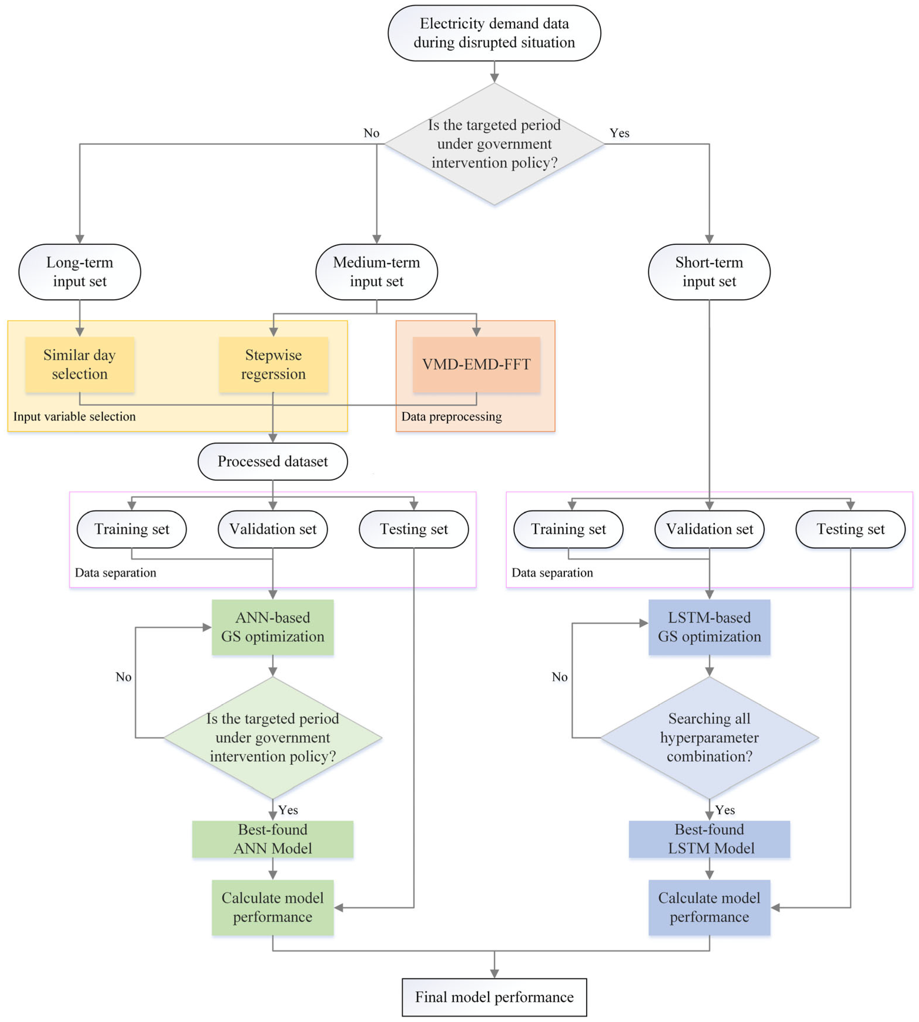
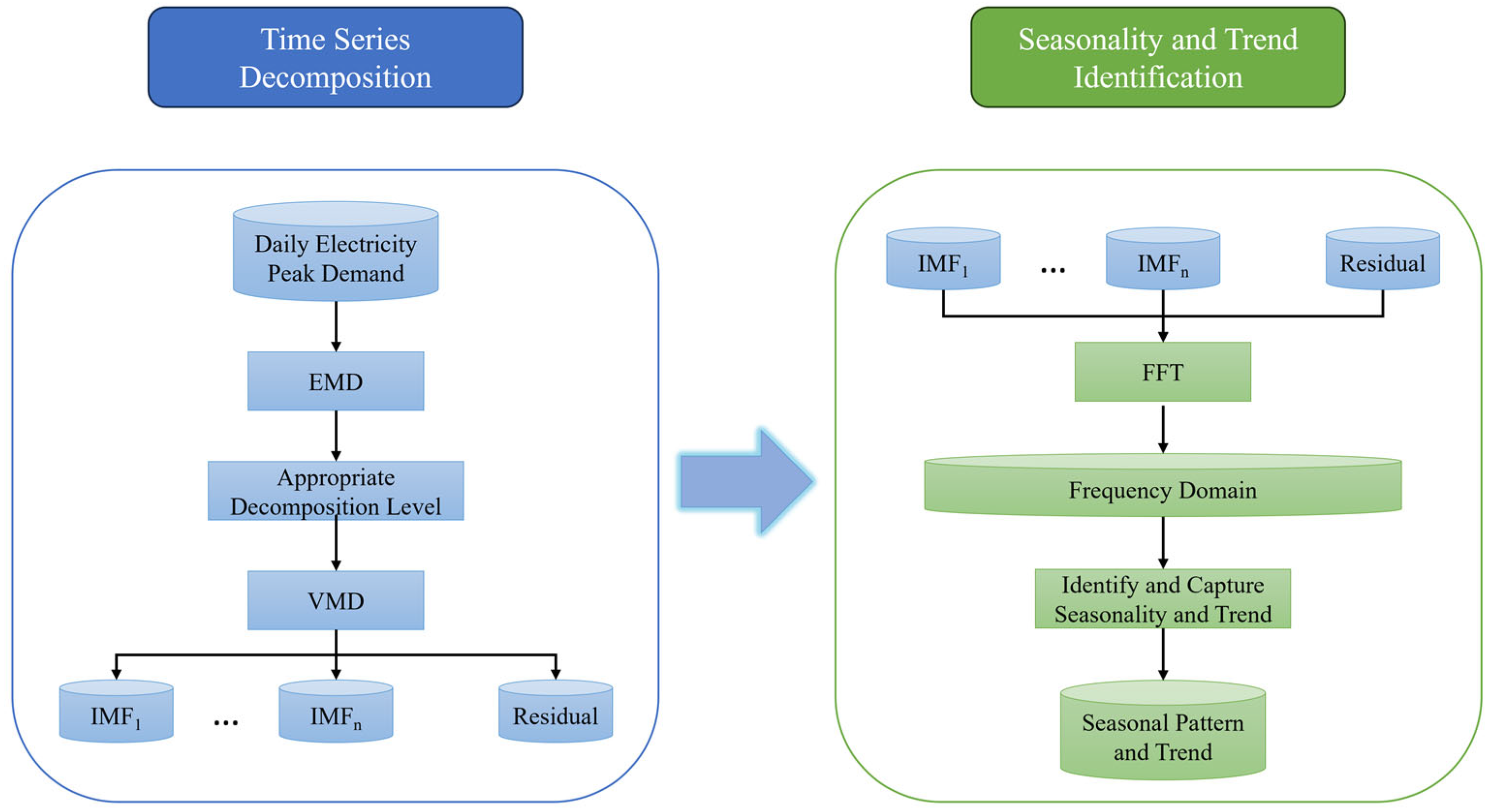
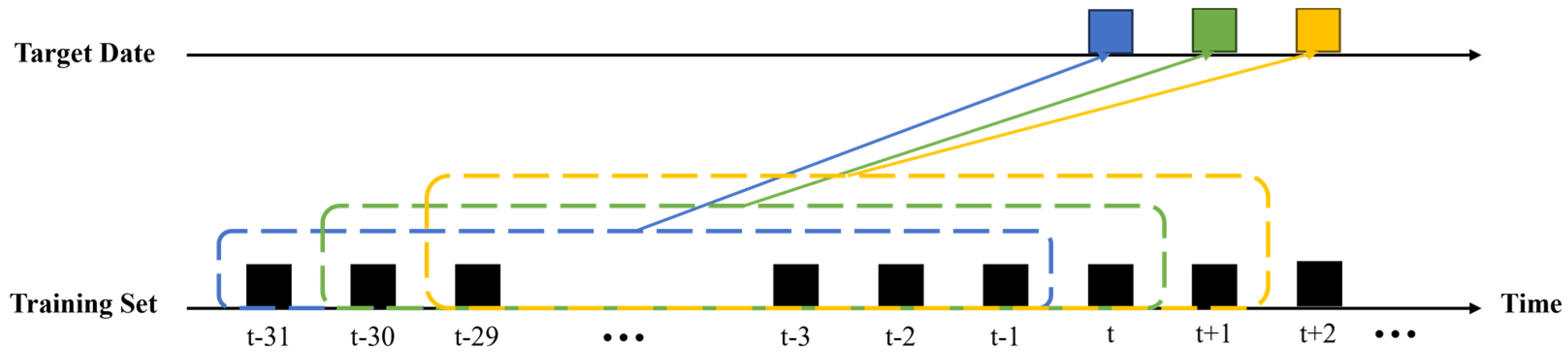
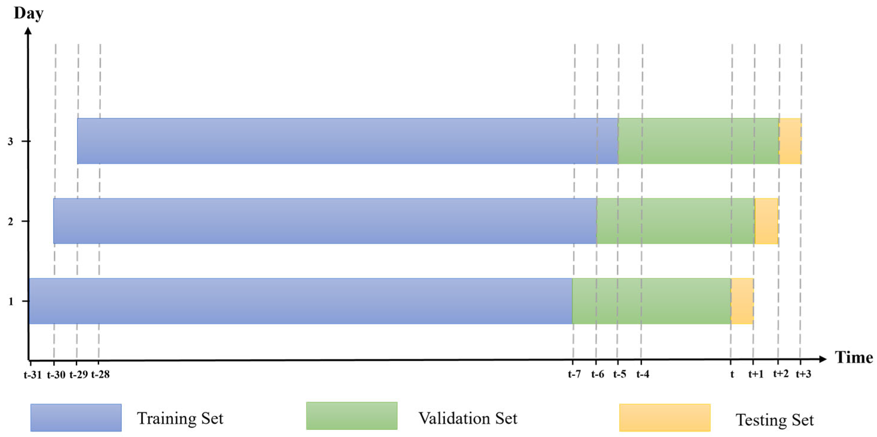
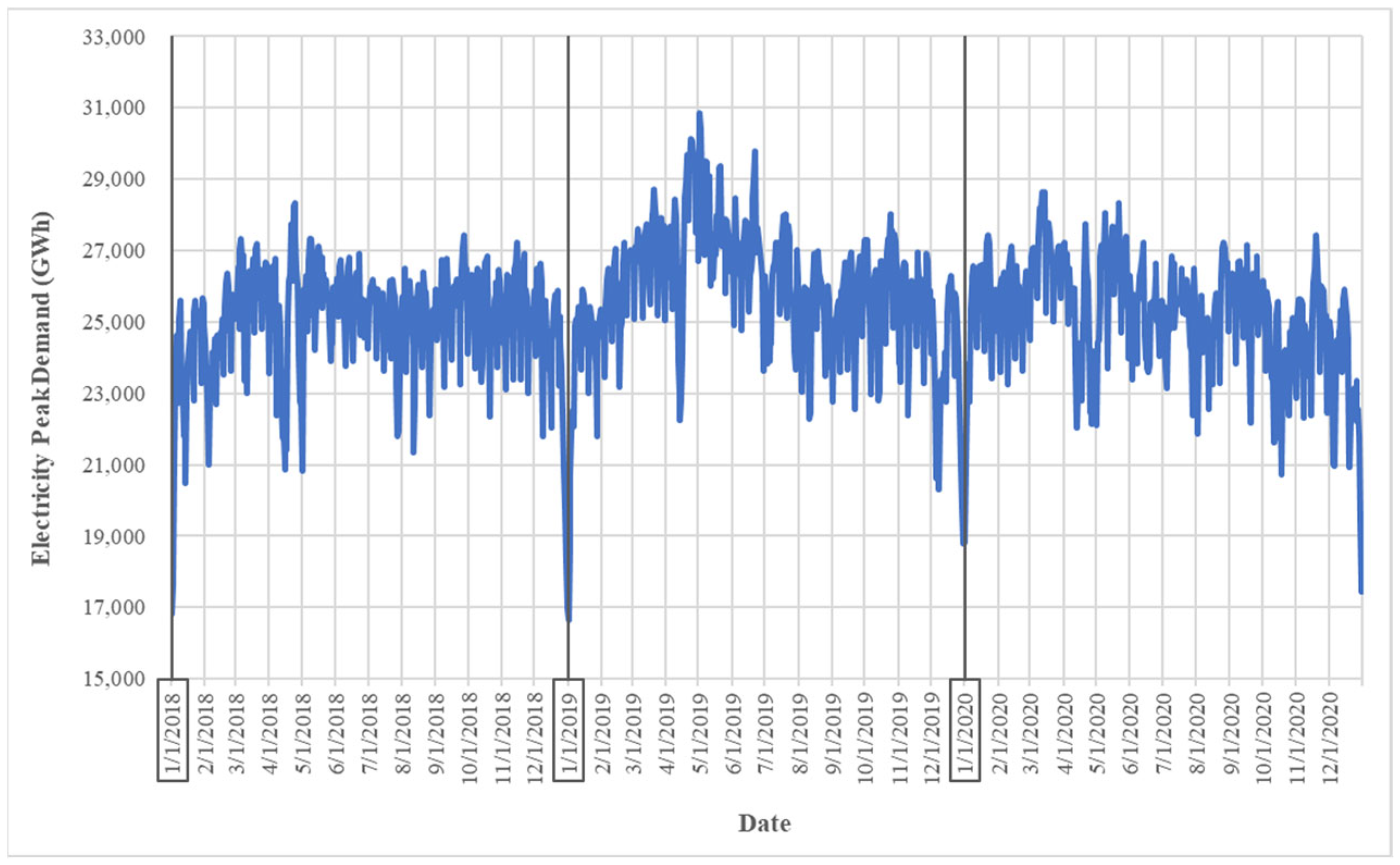
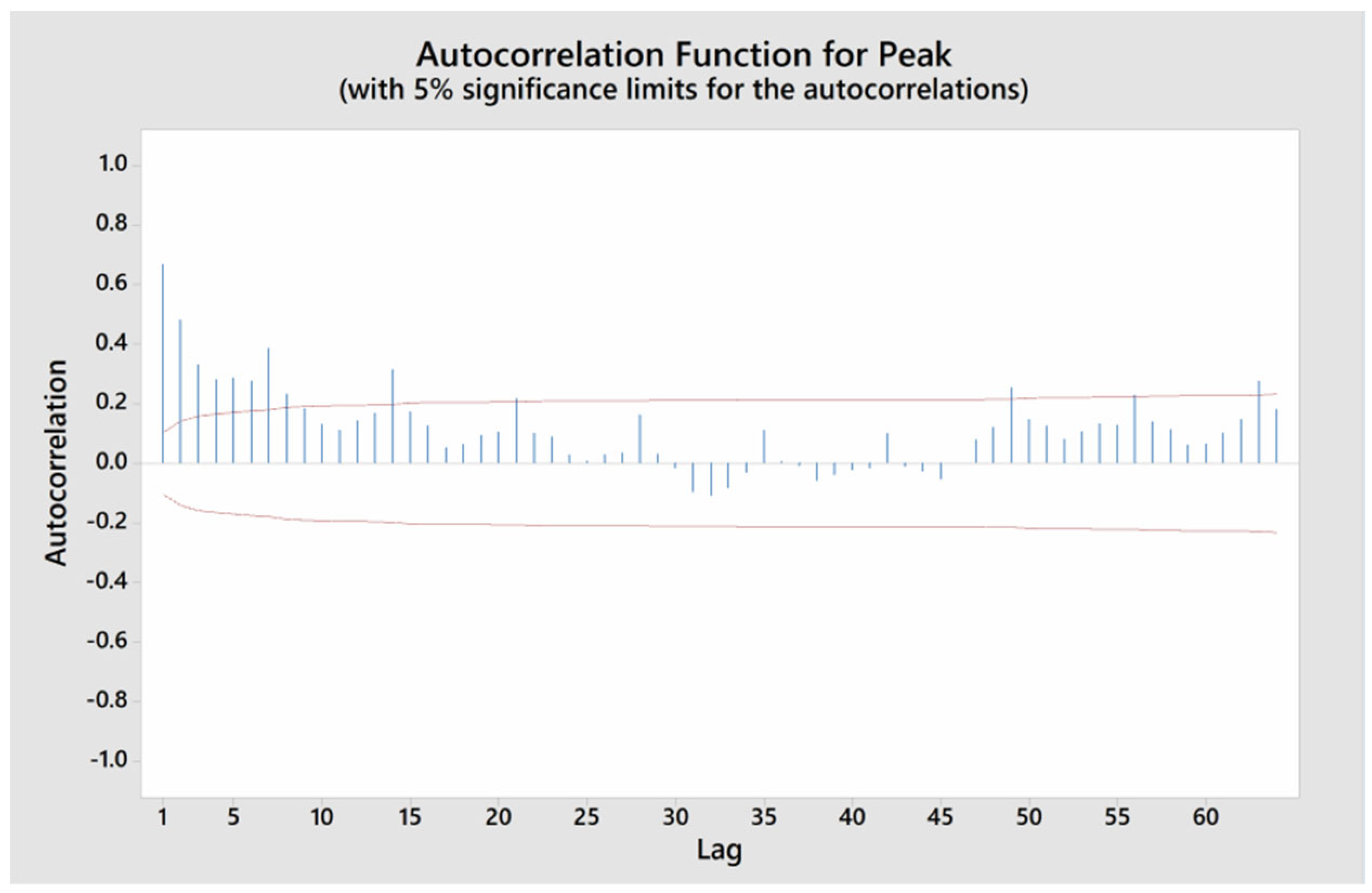

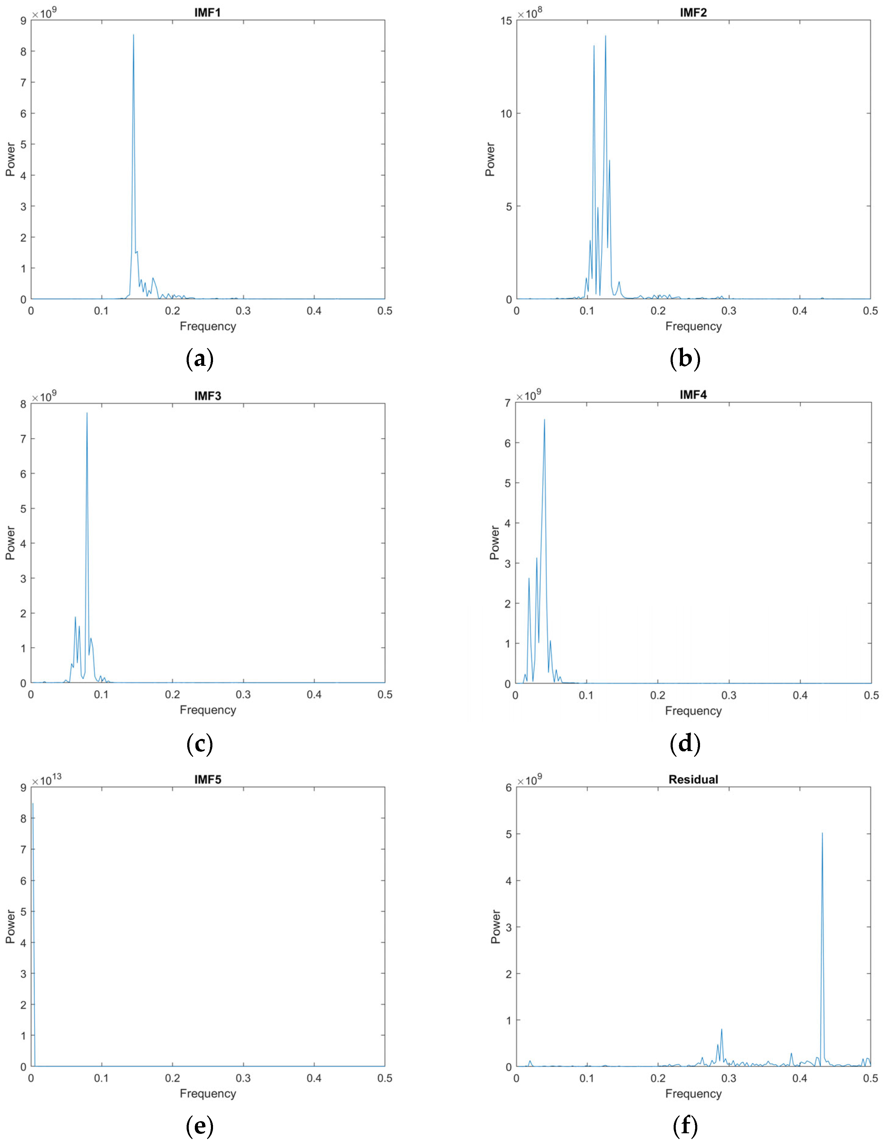
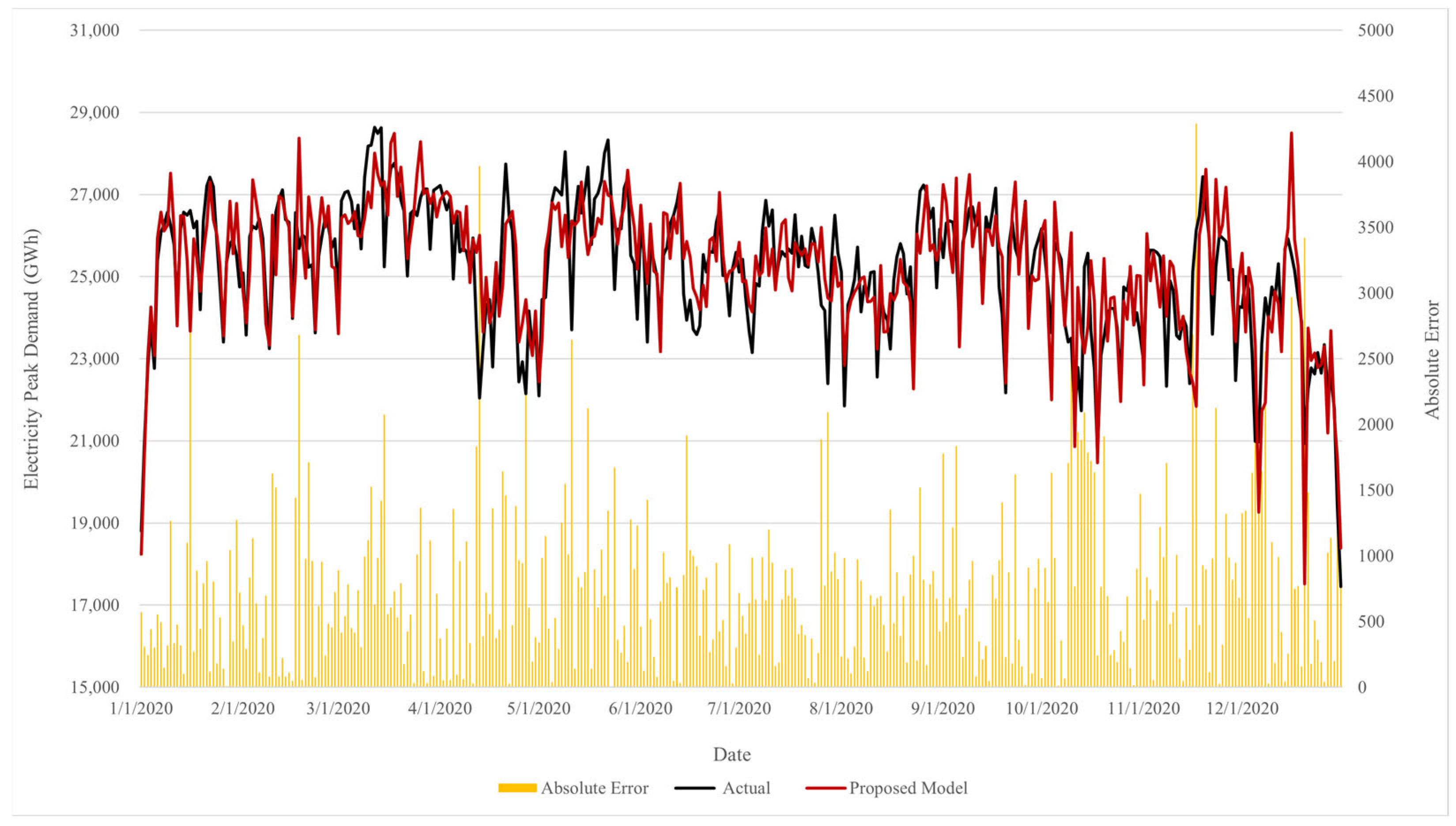

Disclaimer/Publisher’s Note: The statements, opinions and data contained in all publications are solely those of the individual author(s) and contributor(s) and not of MDPI and/or the editor(s). MDPI and/or the editor(s) disclaim responsibility for any injury to people or property resulting from any ideas, methods, instructions or products referred to in the content. |
© 2023 by the authors. Licensee MDPI, Basel, Switzerland. This article is an open access article distributed under the terms and conditions of the Creative Commons Attribution (CC BY) license (https://creativecommons.org/licenses/by/4.0/).