Energy Management in Hybrid Electric Vehicles: A Q-Learning Solution for Enhanced Drivability and Energy Efficiency

Abstract

This study presents a reinforcement-learning-based approach for energy management in hybrid electric vehicles (HEVs). Traditional energy management methods often fall short in simultaneously optimizing fuel economy, passenger comfort, and engine efficiency under diverse driving conditions. To address this, we employed a Q-learning-based algorithm to optimize the activation and torque variation of the internal combustion engine (ICE). In addition, the algorithm underwent a rigorous parameter optimization process, ensuring its robustness and efficiency in varying driving scenarios. Following this, we proposed a comparative analysis of the algorithm’s performance against a traditional offline control strategy, namely dynamic programming. The results in the testing phase performed over ARTEMIS driving cycles demonstrate that our approach not only maintains effective charge-sustaining operations but achieves an average 5% increase in fuel economy compared to the benchmark algorithm. Moreover, our method effectively manages ICE activations, maintaining them at less than two per minute.

1. Introduction

The extensive use of fossil fuel-powered vehicles is widely acknowledged as one of the major contributors to climate change, air, and noise pollution. Governments in various states have announced plans to reduce or even eliminate the sale of conventional vehicles, recognizing the need to address these environmental challenges. Strategies such as energy diversification, fuel decarbonization, and the adoption of electrified solutions are being implemented to tackle these pressing issues. To actively contribute to this evolving scenario, diverse powertrain technologies and alternative fuels can be employed, each with its own advantages and disadvantages. As an example, hydrogen-based solutions face challenges due to the lack of a widespread infrastructure, making them unsuitable for short-term implementation. Similar considerations, along with the imperative to decarbonize the energy production system, should also be taken into account when discussing the adoption of battery-powered vehicles.

In this context, a bridge solution may be represented by hybrid electric vehicles (HEVs). According to several statistical analyses available online, the hybrid market is expected to grow by 20% over the next five years, with the plug-in segment leading the way [1,2]. From a technical point of view, hybrid electric vehicles combine the main advantages of conventional and fully electric vehicles; however, owing to their complex nature, they require sophisticated control logic to obtain a proper energy split among the on-board energy sources, making them widely investigated in the literature. They can be classified according to different classification methods depending on whether they can be recharged by an external source, i.e., PHEVs, or not, i.e., HEVs or whether the traction mechanical power can be provided by the electric motor only, i.e., series configuration, by the electric motor and the engine, i.e., parallel configuration, or complex when either these two configurations are enabled [3,4]. Focusing on the parallel one, in turn, it can be classified according to the position of the electric motor, i.e., P0 if it is connected through a belt to the engine, P1 if directly connected to the engine crankshaft, P2 if in between the engine and the transmission, P3 if post-transmission and P4 if on the opposite axle of the engine. Four operating modes are allowed where in turn the engine (pure thermal) or electric motor (pure electric) provides traction alone, or simultaneously (power-split) or the engine provides traction while recharging the battery (battery charging). Depending on the final application considered (off-line or on-line), several control logics [4,5,6] can be adopted including rule-based [7,8,9,10,11,12], optimization-based [13,14,15,16,17,18,19], data-driven [20,21,22,23,24,25,26,27,28,29,30,31,32] and reinforcement learning (RL) [33,34,35,36,37,38,39,40,41,42,43,44] among the main ones. Rule-based controllers require a substantial calibration effort and they fail to achieve good performance when applied to a driving scenario other than the calibration one. In contrast, optimization-based approaches, such as dynamic programming, not only entail significant computational effort but also rely on prior knowledge of the driving cycle, making them unsuitable for real-time applications. In the classical approaches, a minimization or maximization function is usually defined to enhance, as an example, fuel economy, while ensuring charge-sustaining operation, or a weighted average between carbon dioxide and pollutant emissions [7,8,9,10,11,12,13,14,15,16,17,18,19,20,21,22,23,24,25,26,27,28,29,30,31,32,33,34,35,36,37,38,39,40,41,42,43,44,45,46,47]. However, in this field, a real-time algorithm capable of working in diverse driving scenarios and capable of complying with one or a combination of these goals is still a debated topic especially when customized controllers need to be developed. Reinforcement-learning-based methods, in the last few years, established themselves as a good candidate solution to handle these complex and non-linear control problems. Indeed, the RL agent can be used in a real-time application, avoiding the computational burden typical of optimization-based techniques and the degradation of performance of rule-based solutions when applied to driving scenarios different from the calibration ones [41].

1.1. Related Works

In the domain of HEV energy management, RL holds promise for efficiently distributing power between onboard energy sources to enhance fuel economy while adhering to vehicular component and battery SOC constraints [33,34,35,36,37,38,39,40,41,42,43,44,47]. RL algorithms can be broadly classified into two categories: value-based and policy-based methods. Value-based algorithms exploit learned knowledge to make decisions for a given state. On the other hand, policy-based methods aim to directly model the policy function associated with state–action pairs [48,49,50]. State-of-the-art RL algorithms exhibit various degrees of complexity and computational effort. Notable examples include Q-learning, deep Q-learning, double Q-learning, and actor–critic. By continually interacting with the environment, the Q-learning agent learns and refines its control policy, leveraging the experience gained through exploration-exploitation law. In deep Q-learning, a neural network approximates action Q-values for each state, but caution is needed to prevent over-estimations. Double Q-learning addresses this concern by employing two neural networks, the online and target networks, to separately handle action selection and value estimation [42]. Meanwhile, actor–critic implementations utilize two neural networks: one for policy-based action selection (actor) and another for evaluating action outcomes and estimating value functions (critic) [40]. For instance, Xu et al. [43] employ Q-learning to achieve real-time control, striking a balance between fuel economy and charge sustainability. Chen et al. [44] proposed an energy management control based on model predictive control coupled with double Q-learning to improve the fuel economy and manage the charge-sustaining phase of a power-split PHEV ruling out comfort and drivability requirements. Similar reward considerations are shown in [47] for a deep reinforcement-learning-based energy management with an AMSGrad optimization method and benchmarked with classical dynamic programming. Han et al. [42] propose a double-deep Q-learning algorithm, achieving remarkable improvements in fuel economy while maintaining battery SOC close to a target value. Their approach demonstrates about 7% enhancement over conventional deep Q-learning and nearly 93% of dynamic programming’s performance. Despite the multitude of examples, the current literature tends to overlook the integration of drivability and ride comfort requirements in HEV energy management, especially within the context of RL techniques. Even when multiple deep reinforcement learning algorithms are compared, the focus remains predominantly on well-established metrics such as fuel consumption, battery health degradation, and charge-sustaining SOC [39,40,41,42,43]. The broader considerations of ride quality and comfort requirements often remain unexplored.

1.2. Contribution

In light of the aforementioned literature gaps that predominantly focus on established metrics such as fuel consumption and battery health degradation, in this work, we introduce passenger comfort and ride quality considerations in the design of an RL-based solution for the HEV energy management control problem. To enhance the driving experience, the frequency of ICE de/activations is minimized, while engine torque variation is constrained to a range of 0-80 Nm to ensure smoother engine operation. These parameters are grounded in engineering principles and are designed to simulate the physical constraints inherent to a real-world ICE. The chosen RL algorithm, Q-learning, systematically refines its decision-making process based on historical experiences, gradually improving real-time decision-making. To the best of the authors’ knowledge, no existing examples in the literature showcase the integration of comfort and ride quality considerations within an RL-based energy management control problem. While the recent literature has increasingly moved toward the deployment of sophisticated RL algorithms, often at the expense of an in-depth understanding of the complex physics of the problem domain, our approach takes a different tack. Before adopting more complex methods, we opted to rigorously evaluate the effectiveness of Q-learning, a well-established and state-of-the-art RL technique. This decision was guided by our intent to discern whether a well-understood algorithm could offer a robust solution to the multi-objective optimization problem at hand. In doing so, we aim to establish a meaningful baseline against which to compare the potential benefits and drawbacks of more complex RL strategies, thereby ensuring that any shift toward greater algorithmic complexity is both warranted and advantageous. The key advantages of the proposed approach lie in its ability to adapt to various driving scenarios and account for multiple factors affecting energy consumption, such as driving style, road gradients, engine operation, performance, drivability, and battery state of charge. Considering these factors, the algorithm can dynamically adjust powertrain operation and energy allocation strategies to balance fuel economy, efficient engine operation, passenger comfort, and ride quality. First, the system dynamics of the HEV powertrain are modelled according to a road load approach. To evaluate the effectiveness of the proposed method, extensive simulations are conducted on unknown driving scenarios. Comparative analyses are performed against a conventional offline control strategy, showcasing the tabular Q-learning algorithm’s potential in fuel efficiency and overall system performance. Four perspectives are contributed to the related literature.

• Integration of comfort and ride quality indicators, such as ICE de/activation frequency and torque rate variation constraints, into the energy management control problem using an off-policy RL approach.
• Testing the approach in diverse driving scenarios to validate its applicability and reliability.
• Comparison against a benchmark solution to demonstrate the proposed approach’s performance in fuel and energy efficiency, as well as overall system performance.
• Development of a concise, real-time map for use in automotive control units or similar decision-making systems across different domains.

The rest of this paper is organized as follows: in Section 2 and Section 3, we present the vehicle modelling approach and the problem formulation. In Section 4, we present and discuss the simulation results. Finally, in Section 5, we draw the main conclusions and highlight potential avenues for future research.

2. Vehicle Model

A Jeep Renegade 4xe represented as a parallel P4 architecture, whose scheme is reported in Figure 1, was considered for the purpose of this study [19]. Specifically, the internal combustion engine (ICE) is responsible for powering the front axle, while the electric motor (EM or MGP4) drives the rear axle and is directly connected to the high-voltage battery pack. The main vehicle specifications, obtained by secondary data available online [19], are listed in

Table 1. Vehicle specifications.

Component	Parameter	Value
Vehicle	Mass, $\mathrm{kg}$	1850
	${\mathrm{RL}}_{\mathrm{a}}$, $\mathrm{N}$	125.22
	${\mathrm{RL}}_{\mathrm{b}}$, $\frac{\mathrm{N}}{(\mathrm{m}·\mathrm{s})}$	1.95
	${\mathrm{RL}}_{\mathrm{c}}$, $\frac{\mathrm{N}}{(\mathrm{m}·{\mathrm{s}}^2)}$	0.59
	Tyre radius, m	0.29
Engine	Displacement, $\mathrm{l}$	1.4
	Rated Power, $\mathrm{kW}$	133
	Maximum torque, $\mathrm{Nm}$	270
EM	Rated Power, $\mathrm{kW}$	44
	Maximum torque, $\mathrm{Nm}$	250
Battery	Type	NMC
	Nominal capacity, $\mathrm{Ah}$	28.4
	Nominal voltage, $\mathrm{V}$	400

. The model and algorithm were developed and implemented within the MATLAB^® simulation environment [51].

The HEV powertrain was modelled according to a road load approach as follows:

$$P_{dem}=(ma+0.5\rho c_d{A}_f{v}^2+mg{ϵ}_r)v$$

(1)

where $\mathrm{m}$, $\rho$, ${\mathrm{c}}_{\mathrm{d}}$ and $A_f$ refer to the vehicle mass, air density, drag coefficient and the vehicle frontal area, respectively. The main components such as the electric machine and engine were modelled using quasi-static look-up tables. The torque wheel ${\mathrm{T}}_{\mathrm{w}}$ was computed as a function of the engine torque (${\mathrm{T}}_{\mathrm{eng}}$ or ${\mathrm{T}}_{\mathrm{ICE}}$) and the electric motor torque (${\mathrm{T}}_{\mathrm{EM}}$) considering the driveline.

$$T_w=T_{eng}{\tau }_{g\left(n_{gear}\right)}{\tau }_f{\eta }_g{\eta }_f+T_{EM}{\tau }_r{\eta }_r^{sign\left(T_{EM}\right)}$$

(2)

where the subscripts $\mathrm{g}$, $\mathrm{f}$ and $\mathrm{r}$ refer to the gearbox, the front and rear axle differential efficiencies ($\eta$) or transmission ratios ($\tau$), depending on the case. The gear shifting schedule was determined using a rule-based strategy tied to the road speed, aiming to enhance the vehicle’s performance, approach real-time vehicle usage, and meet passenger comfort requirements [19]. The battery power (${\mathrm{P}}_{\mathrm{batt}}$) was in turn computed considering the electric motor power (${\mathrm{P}}_{\mathrm{EM}}$) and the overall losses of the electric motor (${\mathrm{P}}_{\mathrm{EM},\mathrm{loss}}$) along with the power related to the auxiliaries (${\mathrm{P}}_{\mathrm{aux}}$).

$$P_{batt}=P_{EM}+P_{EM,loss}+P_{aux}$$

(3)

The battery state of charge (SOC) dynamics was evaluated by considering an equivalent open circuit model that consists of an ideal open circuit voltage source in series with an equivalent resistance modelled as in Equation (4):

$$\dot{SOC}=\frac{V_{oc}-\sqrt{V_{oc}^2-4R_{eq}{P}_{batt}}}{2R_{eq}{C}_{batt}}$$

(4)

${\mathrm{V}}_{\mathrm{oc}}$, ${\mathrm{R}}_{\mathrm{eq}}$, and ${\mathrm{C}}_{\mathrm{batt}}$ represent the open circuit voltage, the internal resistance, and the battery capacity, respectively.

3. Problem Formulation

The energy management control problem in hybrid electric vehicles can be framed as a constrained optimization problem over a finite time horizon [3,4]. The optimal control theory provides various approaches to solve this problem by defining a control strategy for a given system that meets a specific optimality criterion. In the problem under analysis, we employed two distinct algorithms: a global optimization algorithm and a reinforcement-learning-based one. The control strategies selected were optimized to ensure the maintenance of the battery SOC within the 18% to 22% range during charge-sustaining mode, owing to the capacity of the PHEV’s battery pack considered for the purpose of this study [19]. In Figure 2, the controller design and its operational scheme are summarized.

3.1. Control Problem

The control system considered in the present research work takes the form:

$$\dot{x}=f(t,x\left(t\right),u\left(t\right)),x\left(t_0\right)=x_0$$

(5)

where the state vector is $\mathrm{x}\left(\mathrm{t}\right)\in \mathrm{X}\subset {\mathbb{R}}^{\mathrm{n}}$, i.e., $\mathrm{x}\left(\mathrm{t}\right)$ has to satisfy a set of inequality constraints $\mathrm{N}\left(\mathrm{x}\right(\mathrm{t}),\mathrm{t})\le 0$; $\mathrm{u}\left(\mathrm{t}\right)\in \mathrm{U}\subset {\mathbb{R}}^{\mathrm{m}}$ is the control vector and $\mathrm{t}\in {\mathbb{R}}^{\mathrm{n}}$ is the time with ${\mathrm{t}}_0$ and ${\mathrm{x}}_0$ representing the initial conditions; in this work, we assumed that the control set is a closed subset of ${\mathbb{R}}^{\mathrm{m}}$ that varies with time. The objective is to find the optimal control law that minimizes a cost functionals of the form [52]:

$$J(t_0,x_0,t_f,u):={\int }_{t_0}^{t_f}L(t,x\left(t\right),u\left(t\right))dt+K(t_f,x_f)$$

(6)

where ${\mathrm{t}}_{\mathrm{f}}$ and ${\mathrm{x}}_{\mathrm{f}}:=\mathrm{x}\left({\mathrm{t}}_{\mathrm{f}}\right)$ are the terminal time and state, $\mathrm{L}$ is the running cost whose domain is $\mathbb{R}\times \mathrm{X}\times \mathrm{U}\to \mathbb{R}$ and $\mathrm{K}$ is the terminal cost whose domain is $\mathbb{R}\times \mathrm{X}\to \mathbb{R}$. In the context of HEVs, the running cost is usually related to fuel consumption whereas the terminal constraint is designed to account for the charge sustainability requirement. The minimization of J is typically subject to multiple constraints, usually associated with physical limitations of powertrain components, the energy stored in the battery, and requirements related to charge sustainability. Specifically, the charge-sustaining constraint ensures that the vehicle keeps its electrical charge without an external source throughout a given driving mission

$$x\left(t_f\right)=x\left(t_0\right),$$

(7)

typically with a certain tolerance to account for practical considerations and to simply maintain energy within predefined boundaries [4]:

$$K(t_f,x_f)=\varphi \left[x\left(t_f\right)-x\left(t_0\right)\right].$$

(8)

In addition, usually, the battery SOC is bound within a certain range to avoid premature ageing phenomena. To include drivability and ride quality requirements, we added a component to the running cost representative of the frequency of ICE de/activations.

3.2. Benchmark Algorithm

We selected dynamic programming (DP), a numerical method for solving multistage decision-making problems, to solve this constrained finite-horizon control problem and we used it as a benchmark against which to compare the performance of the proposed algorithm. Given that DP is a well-established approach commonly employed in HEV energy management control problems, we have chosen to omit a formal definition within this study, reporting here just a summary of the algorithm itself (Algorithm 1). We direct interested readers to refer to established sources for a comprehensive understanding [4,45,52,53,54,55]. We assessed the performance of the DP algorithm on different objective functions, namely:

• A classical approach where fuel economy and charge sustainability are considered;
• A trade-off between fuel economy and drivability/comfort requirements ensuring charge sustaining operation [19].

The primary aim was to formulate a control problem that closely emulates real-world driving priorities, thereby creating a benchmark akin to a high-fidelity scenario.

Algorithm 1 Dynamic programming with terminal constraint

1: Backward Phase: 2: Initialize $V(t_f,x)$ for all states x at the final time step $t_f$ 3: for $t\leftarrow t_f-1$ downto 1 do 4:     for each state x at time t do 5:        Consider all possible control u in state x at time t 6:        Calculate the expected value $V(t,x,u)$ associated with each action 7:        Apply constraints to eliminate infeasible actions 8:        Update the value function $V(t,x)$ for state x at time t based on the calculated values 9:     end for 10: end for 11: Forward Phase: 12: Initialize the optimal policy $\pi (t,x)$ for all states x and time steps t 13: for  $t\leftarrow 1$  to  $t_f-1$  do 14:     for each state x at time t do 15:        Choose the control $u^{*}$ that maximizes $V(t,x,u)$ 16:        Set the policy $\pi (t,x)=u^{*}$ 17:     end for 18: end for 19: Output: Optimal value function $V(t,x)$ and policy $\pi (t,x)$ for all time steps t and states x

3.3. Proposed Solution

Q-learning is said to be an off-policy temporal difference control algorithm. An off-policy method decouples the learning policy from the policy being evaluated, allowing the agent to learn from experiences generated by following a different exploratory policy. This allows the agent to explore the environment more extensively early in the training phase and gradually move towards exploitation as it accumulates knowledge according to an $ϵ$–greedy law [48], which addresses the trade-off between exploration and exploitation. In the present work, the $ϵ$–greedy law assumes the form of an exponential decay function.

$$\begin{array}{cc}\hfill Q(x_k,u_k)& \leftarrow Q(x_k,u_k)\hfill \\ \hfill & +\alpha \left[r_{k+1}+\gamma \underset{u^{\prime }}{max}Q(x_{k+1},u^{\prime })-Q(x_k,u_k)\right]\hfill \end{array}$$

(9)

where $\mathrm{Q}({\mathrm{x}}_{\mathrm{k}},{\mathrm{u}}_{\mathrm{k}})$ represents the Q-value of state–action pair $({\mathrm{x}}_{\mathrm{k}},{\mathrm{u}}_{\mathrm{k}})$, the update rule adjusts this value based on the immediate reward ${\mathrm{r}}_{\mathrm{k}+1}$, the learning rate $\alpha$, and the discounted future reward $\gamma {max}_{{\mathrm{u}}^{\prime }}\mathrm{Q}({\mathrm{x}}_{\mathrm{k}+1},{\mathrm{u}}^{\prime })$, thereby integrating current experience to refine future action-value estimations.

On-policy methods, on the other hand, update the policy based on actions taken during learning, which means that the agent’s policy converges with the observed behaviour during training. Specifically, the Q-value is updated using the action actually taken in the next state, $\mathrm{Q}({\mathrm{x}}_{\mathrm{k}+1},{\mathrm{u}}_{\mathrm{k}+1})$, reflecting a learning approach that assesses and improves upon the policy it employs to make decisions.

$$\begin{array}{cc}\hfill Q(x_k,u_k)& \leftarrow Q(x_k,u_k)\hfill \\ \hfill & +\alpha \left[r_{k+1}\right.\left.+\gamma Q(x_{k+1},u_{k+1})-Q(x_k,u_k)\right]\hfill \end{array}$$

(10)

The rewards an agent receives depend on the control actions and are designed in such a way to be representative of the contribution of each control action to the ultimate goal. In the Q-learning representation, the value function transition, which represents the updated value of the Q–table for a state–action pair resulting from each reward, is stored in a table. By extrapolating the actions corresponding to the highest values for each combination of the state variables, it is possible to create a lookup table of rules for real-time use. The Q–table is updated by adding the learning rate ($\alpha$) multiplied by the temporal difference error, which is the difference between the current Q-value and the sum of the immediate stage cost and the discounted maximum Q-value of the next state, with the discount factor ($\gamma$) as reported in Equation (9). This process enables the agent to iteratively update the Q-values based on observed rewards, transitions, and potential future rewards, gradually improving its policy. Algorithm 2 shows the main algorithm structure.

Algorithm 2 Tabular Q-learning

1: Initialize the Q-values for all state–action pairs in a table form 2: Define the set of allowable actions u(x) for each state x 3: Initialize the current state s and choose an initial action u using an exploration strategy (e.g., epsilon-greedy) 4: for  $N_{episodes}$  do 5:    Take action u, observe the next state $x^{\prime }$ and receive a reward r 6:    Update the $Q_{value}$ for the current state–action pair using the temporal difference learning rule 7:    Choose the next action $u^{\prime }$ using a policy derived from the $Q_{value}$ and the allowable actions for state $x^{\prime }$ 8:    Set $x=x^{\prime }$ and $u=u^{\prime }$ 9: end for 10: Use the trained $Q_{value}$ to make decisions in the environment

Simulation Setup and Q-Learning Based Controller Design

The ICE torque functions as the decision variable $\mathrm{u}$. The state vector $\mathrm{x}$, on the other hand, incorporates the battery SOC, the power required at the wheels, and the ICE torque. Including ICE torque in the state vector is essential for continuously monitoring and regulating its rate of change. This ensures the consistent and gradual modulation of the controlled torque over time and therefore the comfort of the ride. The reward was designed to include three main components: fuel consumption ${\mathrm{m}}_{\mathrm{f}}$, the frequency of ICE de/activations $\left({\mathrm{x}}_3<0\wedge \mathrm{u}>0\right)$, and battery SOC charge sustainability $\left({\mathrm{x}}_{1,\mathrm{ref}}-{\mathrm{x}}_1\right)$.

$$r_t=c_1-\left[c_2·m_f+c_3·\left|x_{1,\mathrm{ref}}-x_1\right|+c_4·\left(x_3<0\wedge u>0\right)\right]$$

(11)

The variables ${\mathrm{x}}_1$ and ${\mathrm{x}}_3$ represent the first and third state variables, respectively. The weights of each term of the reward function $({\mathrm{c}}_2,{\mathrm{c}}_3,{\mathrm{c}}_4)$ were properly adjusted to achieve the best compromise between fuel economy, charge-sustainability, and frequency of ICE de/activations. ${\mathrm{c}}_1$ is a non-negative constant introduced to limit numerical problems during the learning process. In addition, local constraints were imposed on state, control variables, and all the intermediate variables to compute them so as to guarantee the functioning of the vehicle’s main components:

$$\begin{array}{c}\hfill SO{C}_{min}\le SOC\left(t\right)\le SO{C}_{max}\end{array}$$

(12a)

$$\begin{array}{c}\hfill P_{batt,min}\le P_{batt}\left(t\right)\le P_{batt,max}\end{array}$$

(12b)

$$\begin{array}{c}\hfill T_{v,min}\le T_v\left(t\right)\le T_{v,max}\end{array}$$

(12c)

$$\begin{array}{c}\hfill {\omega }_{v,min}\le {\omega }_v\left(t\right)\le {\omega }_{v,max},v=ICE,EM\end{array}$$

(12d)

Table 2. Experiment configuration and parameters for tabular Q-learning.

Parameter	Value
Learning Rate $\alpha$	0.9
Discount Factor $\gamma$	0.99
$ϵ$ greedy law	Exponential decay
Action(s)	{$T_{ICE}$}
State(s)	{SOC, $P_w$, $T_{ICE}$}
Reward Function	$c_1-\left[c_2·m_f+c_3·\left|x_{1,\mathrm{ref}}-x_1\right|+c_4·\left(x_3<0\wedge u>0\right)\right]$

summarizes the parameters and configuration setup of the proposed algorithm.

The Q–table was initialized as a three-dimensional array where each element was sampled independently from a normal distribution, characterized by a mean of ${\mathrm{k}}_1$ and a standard deviation of ${\mathrm{k}}_2$, tuned offline to achieve the desired performance.

The pure electric operating condition was modelled by simulating a fictitious scenario where the internal combustion engine torque was set to a negative value. Consequently, when the controller set ${\mathrm{T}}_{\mathrm{ICE}}=-\mathrm{z}$, it indicates the pure electric mode. During acceleration conditions, a maximum torque variation of 80 Nm within the selected 1 s sample time was permitted, while during braking conditions, a maximum variation of −100 Nm was allowed, so as to enforce the ride quality requirements.

From an algorithmic point of view, the termination condition was established based on a predetermined number of episodes, whereas the early stopping criteria focused on the evaluation of the cumulative reward and on the value of the cumulative discounted return. As a remark, the cumulative reward represents the total sum of the rewards obtained by the agent during the entire learning process without applying any discount.

$$R=\sum _{t=0}^T{r}_t$$

(13)

By measuring the cumulative reward, it is possible to evaluate the overall performance and see if it improves over time. On the other hand, discounted cumulative reward calculates the sum of discounted rewards over time, using a discount factor, represented by gamma.

$$R_{\gamma }=\sum _{t=0}^T{\gamma }^t{r}_t$$

(14)

The discount factor reduces the importance of future rewards compared to immediate ones. For this reason, although it was evaluated as a criterion for assessing the performance of the algorithm and considering early termination, it was not regarded as the primary early termination criterion.

Furthermore, a pure exploitation validation was conducted every 500 episodes to assess the agent’s overall performance and evaluate the learning phase, and the Q–table was saved for testing purposes. The overall algorithmic system design scheme is depicted in Figure 2.

4. Results

4.1. Evaluation Metrics

From a physical point of view, the performance evaluation encompassed several metrics including the cumulative fuel consumption over the driving mission, the frequency of ICE de/activations, and the final state of charge (SOC) of the battery. Specifically, the fuel consumption per unit of distance travelled (L/100 km) was selected as the energy efficiency index; the frequency of ICE activations, measured in occurrences per minute $(1/\min )$, was selected as the passengers’ comfort index; the final SOC (${\mathrm{SOC}}_{\mathrm{f}}$) was selected as the charge-sustaining index.

4.2. DP Results

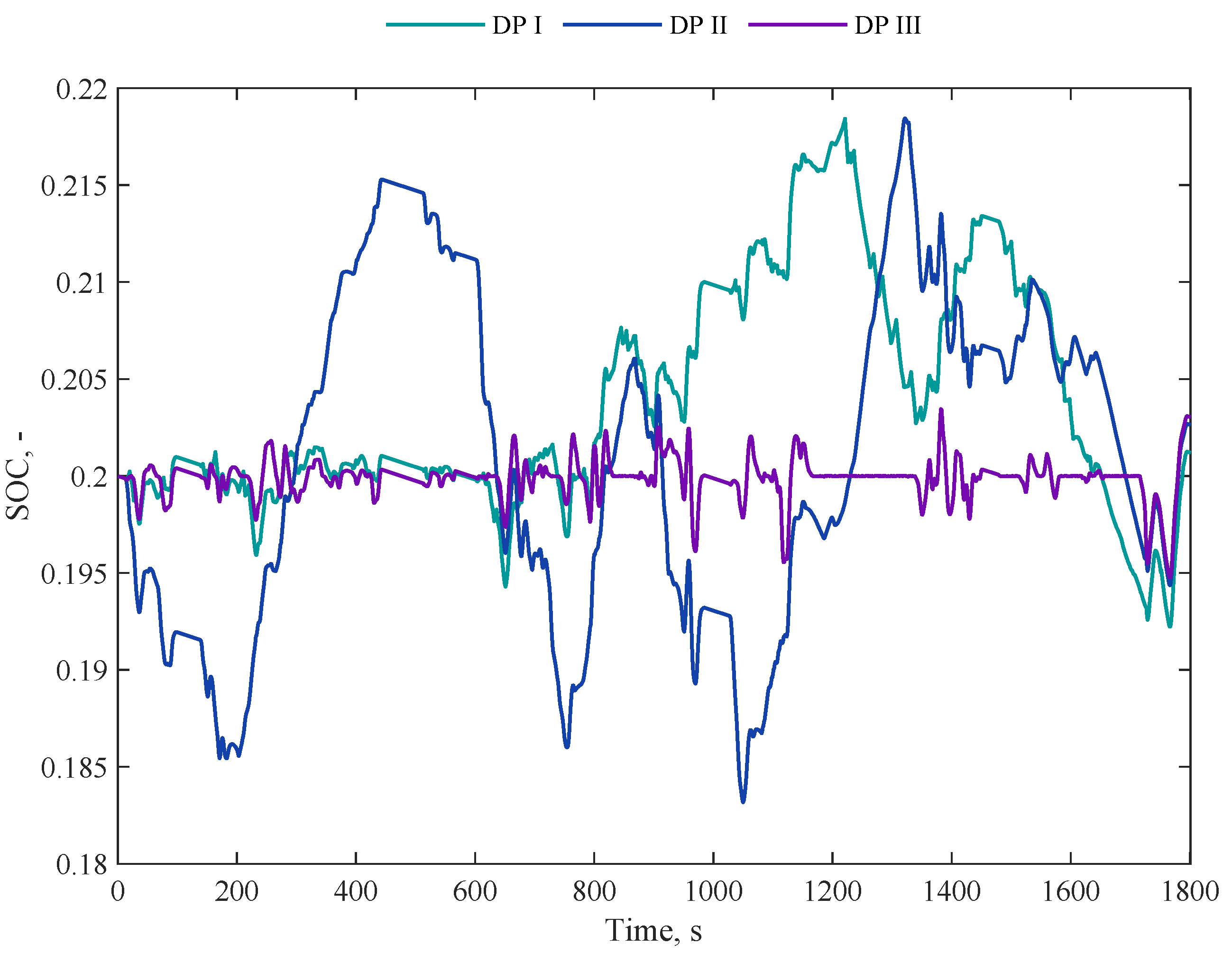
The main results for the WLTP driving cycle, summarized in

Table 3. Performance results for DP algorithm on the WLTP driving cycle.

Label 1 -	FC 2 L/100 km	${\mathbf{f}}_{\mathbf{ICE}}$ 2 1/min	${\mathbf{SOC}}_{\mathbf{f}}$ -	${\mathbf{FC}}_{\mathbf{corr}}$ 2,3 L/100 km
I	6.69	2.1	0.201	6.71
II	7.08	0.13	0.203	7.18
III	7.6	0.07	0.203	7.74

¹ It indicates a specific objective function; ² FC = Fuel consumption; ${\mathrm{f}}_{\mathrm{ICE}}$ = Frequency of ICE activations; ${\mathrm{FC}}_{\mathrm{corr}}$ = Corrected fuel consumption. ³ Correction of fuel consumption to account for SOC variation.

, are presented considering the aforementioned metrics. As outlined in Section 3.2, the algorithm performance was evaluated considering different objective functions accounting for:

• Fuel economy and charge sustainability (I);
• Trade-off between fuel-economy, charge sustainability and drivability (II) [19];
• Same reward function used for the Q-learning learning algorithm (III) (Please refer to Equation (11)).

Complementing this analysis, Figure 3 depicts the SOC trends, showcasing the outcomes of employing different objective functions.

4.3. Comparison Assumptions

To establish a mathematically consistent comparison between two algorithms, they should attempt to solve the same mathematical problem, which in this case includes the same vehicle model, the same objective function, and the same constraints. The off–policy method should converge to the benchmark algorithm we chose, dynamic programming, over an infinite time horizon. Once the two algorithms achieve comparable results in terms of cumulative cost function and cumulative reward function, the comparison should be consistent from a physical point of view as well. However, in practical scenarios, particularly when addressing a multi-objective control problem, identifying a feasible objective function that yields the desired outcomes might be challenging. This is due in part to the fact that the benchmark algorithm allows for the enforcement of a final state, whereas achieving this outcome with the off-policy approach is not straightforward. Consequently, we opted to compare the results obtained from both reinforcement learning (RL) and dynamic programming (DP), utilizing two different objective functions, with a specific emphasis on physics and set goals. Specifically, as shown in the reward function in Table 2, the RL agent faced a penalty based on the SOC value compared to the reference one, a penalty every time it starts the engine, and a term related to fuel consumption throughout the driving mission. On the dynamic programming side, the cost function we selected resulting from the best trade-off among the defined objectives, includes a penalty for the frequency of ICE de/activations, a contribution term for consumption, and a final state constraint [19].

4.4. Correction of Fuel Consumption to Account for SOC Variation with Respect to the Target Value

In practical implementations, when the final SOC does not reach the target value, we corrected the actual value of fuel consumption by accounting for the net amount of energy variation in the battery, as carried out in [4].

$${\dot{m}}_{f,corr}=\dot{m_f}+\theta \Delta SOC$$

(15)

where $\theta$ translates the amount of energy used in the battery into an equivalent fuel consumption considering the ICE efficiency ${\eta }_{\mathrm{ICE}}$ and the fuel lower heating value ${\mathrm{H}}_{\mathrm{f},\mathrm{LHV}}$.

$$\theta =\frac{P_{batt}}{{\eta }_{ICE}·H_{f,LHV}}$$

(16)

4.5. Q-Learning Results and Discussion

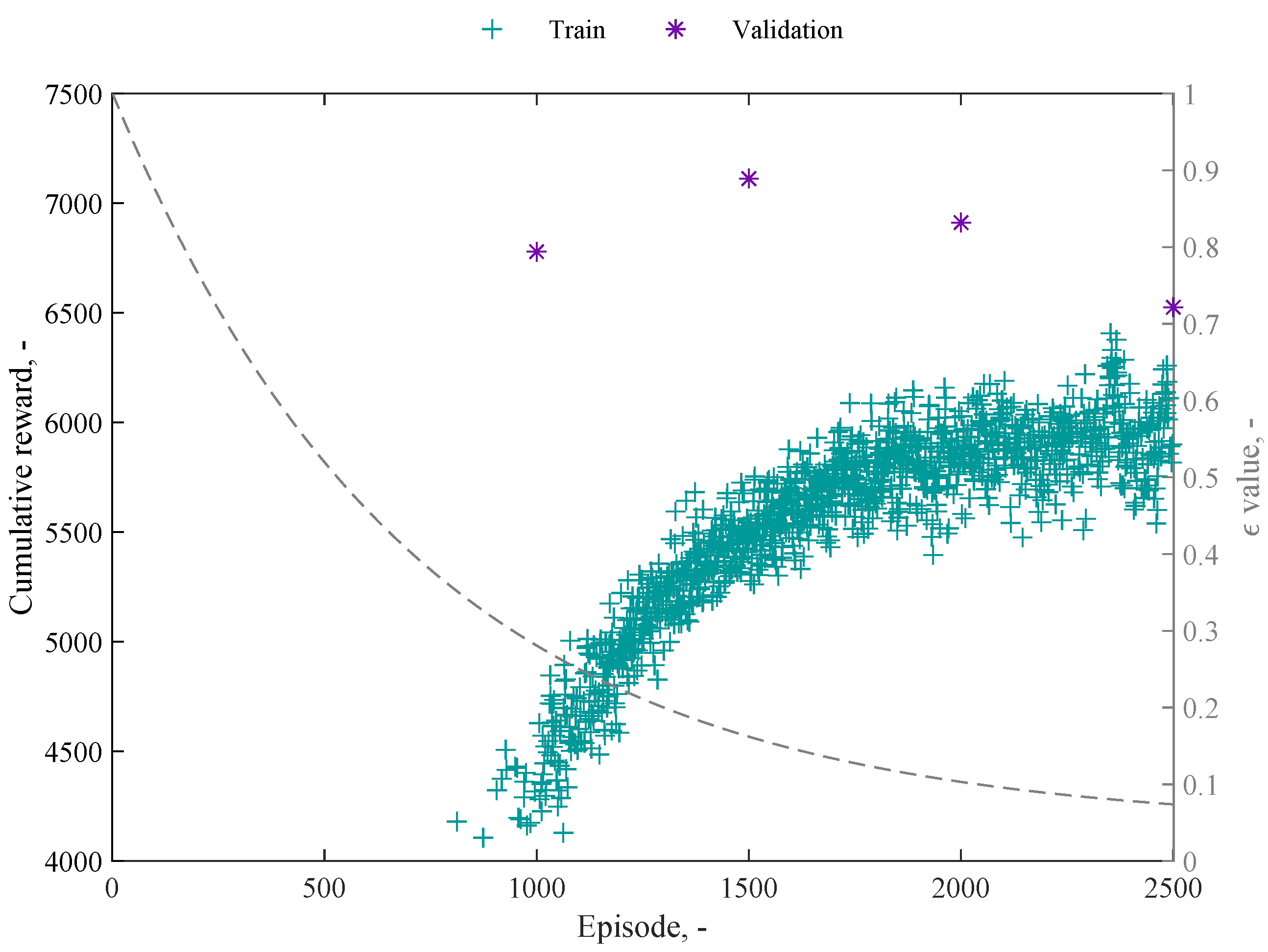
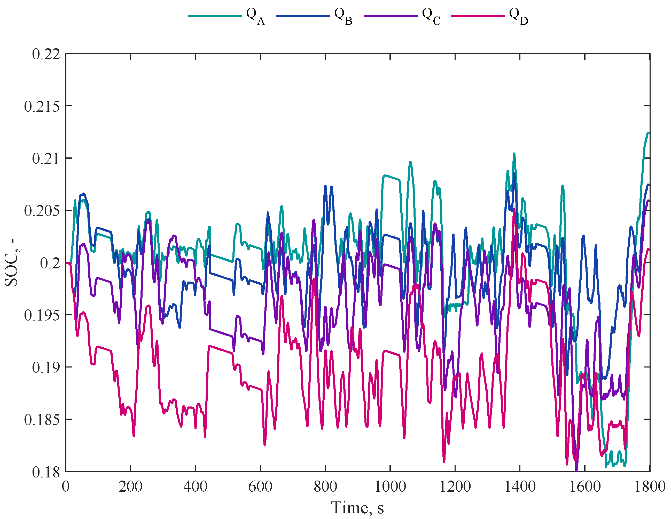
The agent was trained and validated on the worldwide harmonised light vehicle test procedure (WLTP) driving cycle, whereas the testing was performed on the Artemis cycles, including urban (AUDC), rural (ARDC), and motorway (AMDC) segments. The Artemis driving cycles show higher average, and max speeds, and faster acceleration compared to the WLTP cycle. These cycles are designed to adapt to various vehicle types and sizes, incorporating both transient and steady-state driving conditions. The goal is to prove the robustness of the proposed algorithm when applied to driving cycles different from the training one. The performance of the algorithm was assessed considering the cumulative reward, depicted in Figure 4. As observed, despite some fluctuations in the trend caused by the absence of regularization techniques, the algorithm exhibits convergence at approximately episode 1500. The figure showcases four stars representing validation episodes focused on pure exploitation, which are conducted every 500 episodes. Specifically, ${\mathrm{Q}}_{\mathrm{A}}$ refers to episode 1000, ${\mathrm{Q}}_{\mathrm{B}}$ to episode 1500, ${\mathrm{Q}}_{\mathrm{C}}$ to episode 2000, and ${\mathrm{Q}}_{\mathrm{D}}$ to episode 2500. On the other hand, the remaining points correspond to the epsilon-greedy approach, where the exploration percentage exponentially decreases during the training phase. During episodes 1 to 850, there is an empty block indicating that the agent was unable to reach the end of the episode.

The observed discrepancy in cumulative rewards between episode 2500 and episode 1500 provides evidence of a potential local minimum, suggesting a limitation in agent performance. While alternative techniques or strategies could have been explored to mitigate this issue, it is worth noting that both outcomes were on the descending part of the exploration-exploitation law curve, with an $ϵ$ lower than 0.2. Therefore, the current configuration was retained.

The main training, validation, and testing results are summarized in Figure 5 and

Table 4. Performance results for training and validation on the WLTP driving cycle.

${\mathbf{Q}}_{\mathbf{val}}$ 1 -	Episode -	FC 2 L/100 km	${\mathbf{f}}_{\mathbf{ICE}}$ 2 1/min	${\mathbf{SOC}}_{\mathbf{f}}$	${\mathbf{FC}}_{\mathbf{corr}}$ 2,3 L/100 km
${\mathrm{Q}}_{\mathrm{A}}$	1000	7.62	1.63	0.212	9.89
${\mathrm{Q}}_{\mathrm{B}}$	1500	7.59	1	0.207	8.39
${\mathrm{Q}}_{\mathrm{C}}$	2000	7.56	1.17	0.206	8.07
${\mathrm{Q}}_{\mathrm{D}}$	2500	7.53	0.8	0.201	7.55

¹ It indicates a specific pure-exploitation validation episode; ² FC = Fuel consumption; ${\mathrm{f}}_{\mathrm{ICE}}$ = Frequency of ICE activations; ${\mathrm{FC}}_{\mathrm{corr}}$ = Corrected fuel consumption. ³ Correction of fuel consumption to account for SOC variation.

,

Table 5. Comparative performance analysis during the WLTP validation phase for the proposed algorithm and DP.

	Fuel Consumption % Difference
${\mathbf{Q}}_{\mathbf{val}}$ 1	w.r.t. 2 ${\mathbf{DP}}_{\mathbf{I}}$	${\mathbf{DP}}_{\mathbf{II}}$	w.r.t. ${\mathbf{DP}}_{\mathbf{III}}$
${\mathrm{Q}}_{\mathrm{A}}$	+13.9	+7.6	+0.2
${\mathrm{Q}}_{\mathrm{B}}$	+13.45	+7.2	−0.13
${\mathrm{Q}}_{\mathrm{C}}$	+13	+6.78	−0.53
${\mathrm{Q}}_{\mathrm{D}}$	+12.56	+6.35	−0.92
	Corrected Fuel Consumption % Difference
${\mathbf{Q}}_{\mathbf{val}}$	w.r.t.  ${\mathbf{DP}}_{\mathbf{I}}$	w.r.t. ${\mathbf{DP}}_{\mathbf{II}}$	w.r.t. ${\mathbf{DP}}_{\mathbf{III}}$
${\mathrm{Q}}_{\mathrm{A}}$	+46	+37.7	+27.8
${\mathrm{Q}}_{\mathrm{B}}$	+25	+16.85	+8.4
${\mathrm{Q}}_{\mathrm{C}}$	+20.27	+12.39	+4.26
${\mathrm{Q}}_{\mathrm{D}}$	+12.52	+5.15	−2.45
	Frequency of ICE de/Activations Compared to DP
${\mathbf{Q}}_{\mathbf{val}}$	w.r.t. ${\mathbf{DP}}_{\mathbf{I}}$	w.r.t. ${\mathbf{DP}}_{\mathbf{II}}$	w.r.t. ${\mathbf{DP}}_{\mathbf{III}}$
${\mathrm{Q}}_{\mathrm{A}}$	−0.47	+1.5	+1.56
${\mathrm{Q}}_{\mathrm{B}}$	−1.1	+0.87	+0.93
${\mathrm{Q}}_{\mathrm{C}}$	−0.93	+1.04	+1.1
${\mathrm{Q}}_{\mathrm{D}}$	−1.3	+0.67	+0.73

¹ It indicates a specific pure-exploitation validation episode; ² with respect to.

and

Table 6. Performance results: training on the WLTP driving cycle and testing on an unknown driving cycle.

${\mathbf{Q}}_{\mathbf{val}}$ 1 -	Cycle -	FC 2 L/100 km	${\mathbf{f}}_{\mathbf{ICE}}$ 2 1/min	${\mathbf{SOC}}_{\mathbf{f}}$ -	${\mathbf{FC}}_{\mathbf{corr}}$ 2,3 L/100 km
${\mathrm{Q}}_{\mathrm{B}}$	AUDC	5.77	0.66	0.2	5.77
${\mathrm{Q}}_{\mathrm{B}}$	ARDC	6.74	1.72	0.2	6.74
${\mathrm{Q}}_{\mathrm{B}}$	AMDC	10.87	1.24	0.202	10.91
${\mathrm{Q}}_{\mathrm{D}}$	AUDC	4.96	0.483	0.187	16.26
${\mathrm{Q}}_{\mathrm{D}}$	ARDC	6.38	1.22	0.192	7.75
${\mathrm{Q}}_{\mathrm{D}}$	AMDC	10.42	0.67	0.192	11.15

¹ It indicates a specific pure-exploitation validation episode; ² FC = Fuel consumption; ${\mathrm{f}}_{\mathrm{ICE}}$ = Frequency of ICE activations; ${\mathrm{FC}}_{\mathrm{corr}}$ = Corrected fuel consumption. ³ Correction of fuel consumption to account for SOC variation.

, respectively. The labels indicate the different Q–tables obtained through the pure exploitation episodes. The average fuel consumption achieved during the training and validation processes is approximately 7.58 L/100 km, ranging from 7.62 L/100 km in episode 1000 to 7.53 L/100 km in episode 2500. The average frequency of ICE de/activations is approximately 1.15 $1/\min$, with variations from 1.63 $1/\min$ in episode 1000 to 0.8 $1/\min$ in episode 2500. On average we obtain a final state of charge (${\mathrm{SOC}}_{\mathrm{f}}$) of approximately 0.207, ranging from 0.212 in episode 1000 to 0.201 in episode 2500.

To enhance result comprehension, Table 5 provides a comprehensive summary of performance in relation to the DP algorithm with different objective functions. Among the analyzed results from dynamic programming, ${\mathrm{DP}}_{\mathrm{II}}$ stands out as the one that effectively balances fuel consumption, charge sustainability, and drivability. On average, the different episodes of pure exploitation regarding fuel consumption exhibit a mean deviation below 7%, whereas in terms of engine activations, on average they occur approximately 9 times as frequently. On the final SOC side, the comparison was not performed because starting from ${\mathrm{Q}}_{\mathrm{B}}$, there is a percentage deviation of 3.5% from the target, which we considered within acceptable tolerance ranges.

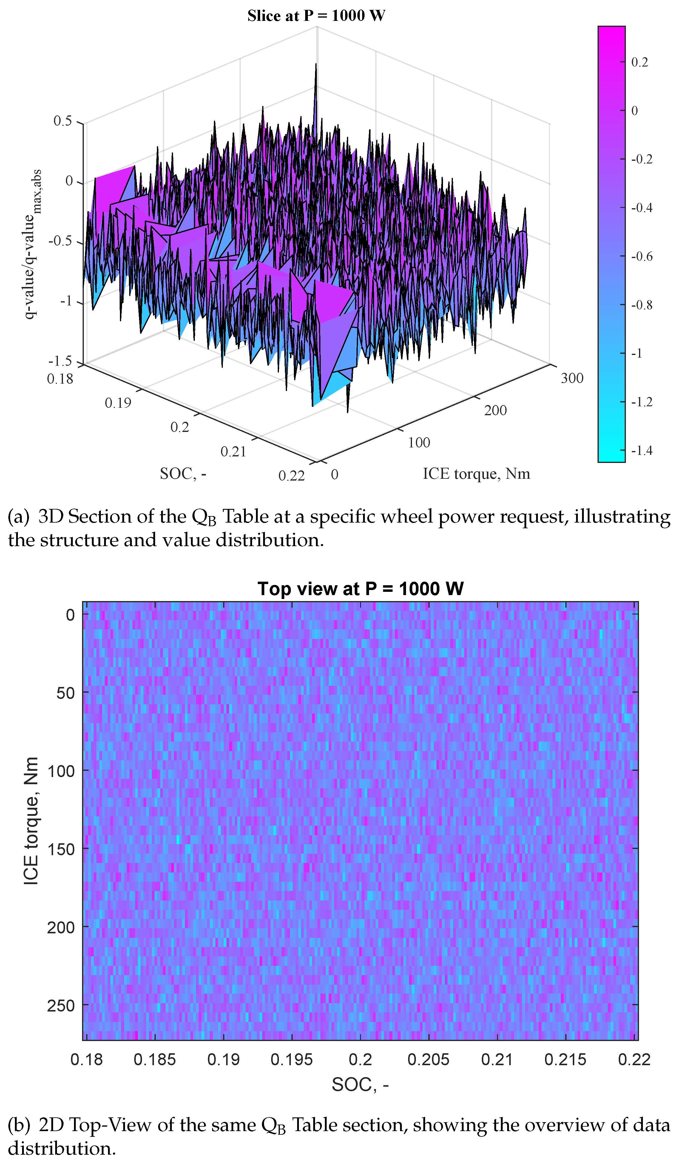
The Q–table was initialized as a three-dimensional array and each element was independently sampled from a normal distribution, characterized by a certain mean and standard deviation. For the sake of completeness, we reported in Figure 6a sliced view at a specific wheel power request for the ${\mathrm{Q}}_{\mathrm{B}}$ table to give the reader a visual representation of the Q–table. This includes a 3D visualization in Figure 6a showcasing the distinct shape of the Q–table in a particular section, as well as a 2D top-view representation in Figure 6b to provide an overview of its contents and stored values.

For the testing phase on the three Artemis driving cycles, we selected the two Q–tables that lead to the highest and lowest cumulative reward, namely ${\mathrm{Q}}_{\mathrm{B}}$ and ${\mathrm{Q}}_{\mathrm{D}}$. They both achieve a final SOC within the feasible range of 0.18–0.22, with ${\mathrm{Q}}_{\mathrm{B}}$ showing higher proximity to the target value. However, ${\mathrm{Q}}_{\mathrm{B}}$ exhibits higher fuel consumption and frequency of ICE activations compared to ${\mathrm{Q}}_{\mathrm{D}}$.

Specifically, for the urban driving cycle (AUDC), ${\mathrm{Q}}_{\mathrm{B}}$ consumes 5.77 L/100 km, approximately 16.33% higher than ${\mathrm{Q}}_{\mathrm{D}}$’s fuel consumption of 4.96 L/100 km. Additionally, ${\mathrm{Q}}_{\mathrm{B}}$ has a higher frequency of ICE activations of 0.66 $1/\min$, representing a 36.81% increase compared to ${\mathrm{Q}}_{\mathrm{D}}$’s frequency of 0.483 $1/\min$.

For the rural driving cycle (ARDC) and the motorway one (AMDC), ${\mathrm{Q}}_{\mathrm{B}}$ shows an increase in fuel consumption of approximately 5.6% and 4.3% respectively, compared to the ${\mathrm{Q}}_{\mathrm{D}}$. Additionally, ${\mathrm{Q}}_{\mathrm{B}}$ exhibits higher frequencies of ICE de/activations, with a 40% increase for ARDC and an 85% increase for AMDC.

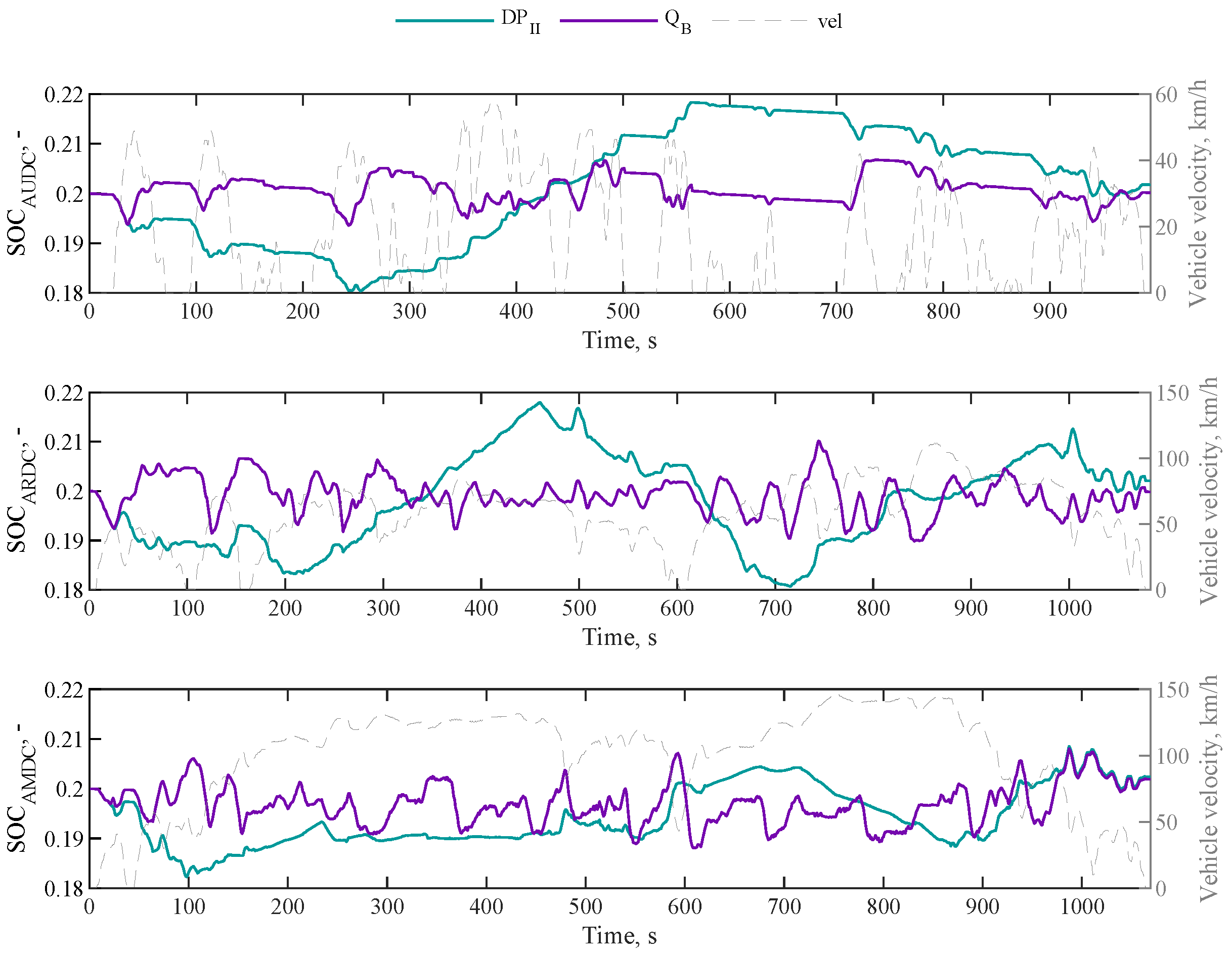
Adopting a conservative approach for the final comparison, the results of Artemis cycles of ${\mathrm{Q}}_{\mathrm{B}}$ were compared to those of ${\mathrm{DP}}_{\mathrm{II}}$, which offers the best trade-off among fuel consumption, the frequency of ICE de/activations, and charge sustainability (

Table 7. Performance results for ${\mathrm{DP}}_{{\mathrm{II}}^1}$ algorithm on the Artemis driving cycles.

Cycle -	FC 1 L/100 km	${\mathbf{f}}_{\mathbf{ICE}}$ 1 1/min	${\mathbf{SOC}}_{\mathbf{f}}$ -	${\mathbf{FC}}_{\mathbf{corr}}$ 1,2 L/100 km
AUDC	5.75	0.121	0.2018	5.97
ARDC	6.27	0.167	0.202	6.36
AMDC	10.1	0.06	0.202	10.17

¹ FC = Fuel consumption; ${\mathrm{f}}_{\mathrm{ICE}}$ = Frequency of ICE activations; ${\mathrm{FC}}_{\mathrm{corr}}$ = Corrected fuel consumption. ² Correction of fuel consumption to account for SOC variation.

and

Table 8. Comparative performance analysis of ${\mathrm{Q}}_{{\mathrm{B}}^2}$ and ${\mathrm{DP}}_{{\mathrm{II}}^1}$ during the ARTEMIS testing phase.

Cycle -	FC 1 L/100 km	${\mathbf{f}}_{\mathbf{ICE}}$ 1 1/min	${\mathbf{FC}}_{\mathbf{corr}}$ 1,2 L/100 km	${\mathbf{SOC}}_{\mathbf{f}}$ -
AUDC	5.77	0.66	5.77	0.201
w.r.t. 3 ${\mathrm{DP}}_{\mathrm{II}}$	+0.34%	+0.54	−3.35	-
ARDC	6.74	1.72	6.74	0.1998
w.r.t. ${\mathrm{DP}}_{\mathrm{II}}$	+7.49%	+1.55	+5.97	-
AMDC	10.87	1.23	10.91	0.2019
w.r.t. ${\mathrm{DP}}_{\mathrm{II}}$	+7.62%	+1.17	+ 7.27	-

¹ FC = Fuel consumption; ${\mathrm{f}}_{\mathrm{ICE}}$ = Frequency of ICE activations; ${\mathrm{FC}}_{\mathrm{corr}}$ = Corrected fuel consumption. ² Correction of fuel consumption to account for SOC variation. ³ with respect to.

). On the fuel economy side, the proposed algorithm obtains an average increase of around 5%, whereas on the frequency of ICE activations side, we have an average frequency of around 12 times higher. The best performances are observed for the AUDC cycle, and the worst for the AMDC cycle. Figure 7 shows the results in terms of SOC for both ${\mathrm{DP}}_{\mathrm{II}}$ and ${\mathrm{Q}}_{\mathrm{B}}$ for AUDC (top), ARDC (middle) and AMDC (bottom) cycles. Similarly, Figure 8 shows the results in terms of ICE torque. During the testing phase, the proposed algorithm demonstrates the ability to maintain the charge-sustaining behaviour even on unknown driving cycles. It achieves a fuel economy comparable to the benchmark algorithm optimized for the specific driving mission while keeping the frequency of ICE de/activations below 2 per minute.

5. Conclusions

The present paper showed the potentiality of reinforcement learning in the form of tabular Q-learning in the HEV energy management control problem when the charge-sustaining phase, fuel economy, comfort and engine operation requirements are considered. The system dynamics of the HEV powertrain were modelled according to a road load approach. A pure exploitation validation of the Q-learning algorithm was conducted every 500 episodes to assess the agent’s overall performance and evaluate the learning phase, and the Q–table was saved for testing purposes. The average fuel consumption achieved during the training and validation processes was approximately 7.58 L/100 km, ranging from 7.62 L/100 km in episode 1000 to 7.53 L/100 km in episode 2500. The average frequency of ICE de/activations was approximately 1.15 $1/\min$, with variations from 1.63 $1/\min$ in episode 1000 to 0.8 $1/\min$ in episode 2500. On average, we obtained a final state of charge (${\mathrm{SOC}}_{\mathrm{f}}$) of approximately 0.207, ranging from 0.212 in episode 1000 to 0.201 in episode 2500. To evaluate the effectiveness of the proposed approach, extensive simulations were conducted on unknown driving scenarios. Specifically, for the testing phase on the three Artemis driving cycles, we selected the two Q–tables that lead to the highest and lowest cumulative reward, namely ${\mathrm{Q}}_{\mathrm{B}}$ and ${\mathrm{Q}}_{\mathrm{D}}$. They both achieved a final SOC within the feasible range of 0.18–0.22, with ${\mathrm{Q}}_{\mathrm{B}}$ showing higher proximity to the target value. However, ${\mathrm{Q}}_{\mathrm{B}}$ exhibits higher fuel consumption and frequency of ICE activations compared to ${\mathrm{Q}}_{\mathrm{D}}$. Comparative analyses were performed against a conventional offline control strategy, showcasing the tabular Q-learning algorithm’s potential in fuel efficiency and overall system performance. During the testing phase, the proposed algorithm demonstrated the ability to maintain the charge-sustaining behaviour, even on unknown driving cycles. It achieved a fuel economy comparable to the benchmark algorithm, optimized for that specific driving mission while keeping the frequency of ICE de/activations below 2 per minute. In particular, it achieved an average fuel economy increase of approximately 5% compared to the benchmark algorithm. Additionally, it demonstrated an average frequency of approximately 12 times higher for the frequency of ICE activations side. The next steps include a validation in a Hardware-in-the-Loop (HIL) simulation environment, with a comparison to commonly used algorithms.

References

1. MordorIntelligence. Hybrid Vehicle Market Analysis—Industry Report—Trends, Size & Share. Available online: https://www.mordorintelligence.com/industry-reports/hybrid-vehicle-market (accessed on 30 October 2022).
2. Lelli, E.; Musa, A.; Batista, E.; Misul, D.A.; Belingardi, G. On-Road Experimental Campaign for Machine Learning Based State of Health Estimation of High-Voltage Batteries in Electric Vehicles. Energies 2023, 16, 4639. [Google Scholar] [CrossRef]
3. Guzzella, L.; Sciarretta, A. Vehicle Propulsion Systems: Introduction to Modeling and Optimization; Springer: Berlin/Heidelberg, Germany, 2007. [Google Scholar] [CrossRef]
4. Onori, S.; Serrao, L.; Rizzoni, G. Hybrid Electric Vehicles: Energy Management Strategies; Springer: London, UK, 2016. [Google Scholar]
5. Wirasingha, S.G.; Emadi, A. Classification and Review of Control Strategies for Plug-In Hybrid Electric Vehicles. IEEE Trans. Veh. Technol. 2011, 60, 111–122. [Google Scholar] [CrossRef]
6. Pisu, P.; Rizzoni, G. A Comparative Study Of Supervisory Control Strategies for Hybrid Electric Vehicles. IEEE Trans. Control. Syst. Technol. 2007, 15, 506–518. [Google Scholar] [CrossRef]
7. Jalil, N.; Kheir, N.; Salman, M. A rule-based energy management strategy for a series hybrid vehicle. In Proceedings of the 1997 American Control Conference (Cat. No.97CH36041), Albuquerque, NM, USA, 6 June 1997; Volume 1, pp. 689–693. [Google Scholar] [CrossRef]
8. Hofman, T.; Steinbuch, M.; Druten, R.; Serrarens, A. A Rule-based energy management strategies for hybrid vehicles. Int. J. Electr. Hybrid Veh. 2007, 1, 71–94. [Google Scholar] [CrossRef]
9. Banvait, H.; Anwar, S.; Chen, Y. A rule-based energy management strategy for Plug-in Hybrid Electric Vehicle (PHEV). In Proceedings of the 2009 American Control Conference, St. Louis, MO, USA, 10–12 June 2009; pp. 3938–3943. [Google Scholar] [CrossRef]
10. Hofman, T.; Steinbuch, M.; van Druten, R.; Serrarens, A. Rule-Based Energy Management Strategies for Hybrid Vehicle Drivetrains: A Fundamental Approach in Reducing Computation Time. IFAC Proc. Vol. 2006, 39, 740–745. [Google Scholar] [CrossRef]
11. Goerke, D.; Bargende, M.; Keller, U.; Ruzicka, N.; Schmiedler, S. Optimal Control based Calibration of Rule-Based Energy Management for Parallel Hybrid Electric Vehicles. SAE Int. J. Altern. Powertrains 2015, 4, 178–189. [Google Scholar] [CrossRef]
12. Peng, J.; He, H.; Xiong, R. Rule based energy management strategy for a series–parallel plug-in hybrid electric bus optimized by dynamic programming. Appl. Energy 2017, 185, 1633–1643. [Google Scholar] [CrossRef]
13. Sciarretta, A.; Guzzella, L. Control of hybrid electric vehicles. IEEE Control. Syst. Mag. 2007, 27, 60–70. [Google Scholar] [CrossRef]
14. Xie, S.; Hu, X.; Xin, Z.; Brighton, J. Pontryagin’s Minimum Principle based model predictive control of energy management for a plug-in hybrid electric bus. Appl. Energy 2019, 236, 893–905. [Google Scholar] [CrossRef]
15. Kim, N.; Cha, S.; Peng, H. Optimal Control of Hybrid Electric Vehicles Based on Pontryagin’s Minimum Principle. IEEE Trans. Control. Syst. Technol. 2011, 19, 1279–1287. [Google Scholar] [CrossRef]
16. Musardo, C.; Rizzoni, G.; Guezennec, Y.; Staccia, B. A-ECMS: An Adaptive Algorithm for Hybrid Electric Vehicle Energy Management. Eur. J. Control. 2005, 11, 509–524. [Google Scholar] [CrossRef]
17. Onori, S.; Serrao, L.; Rizzoni, G. Adaptive equivalent consumption minimization strategy for hybrid electric vehicles. In Proceedings of the Dynamic Systems and Control Conference, Cambridge, MA, USA, 12–15 September 2010; Volume 44175, pp. 499–505. [Google Scholar]
18. Delprat, S.; Lauber, J.; Guerra, T.; Rimaux, J. Control of a parallel hybrid powertrain: Optimal control. IEEE Trans. Veh. Technol. 2004, 53, 872–881. [Google Scholar] [CrossRef]
19. Anselma, P.G. Rule-based Control and Equivalent Consumption Minimization Strategies for Hybrid Electric Vehicle Powertrains: A Hardware-in-the-loop Assessment. In Proceedings of the 2022 IEEE 31st International Symposium on Industrial Electronics (ISIE), Anchorage, AK, USA, 1–3 June 2022; pp. 680–685. [Google Scholar] [CrossRef]
20. Millo, F.; Rolando, L.; Tresca, L.; Pulvirenti, L. Development of a neural network-based energy management system for a plug-in hybrid electric vehicle. Transp. Eng. 2023, 11, 100156. [Google Scholar] [CrossRef]
21. Finesso, R.; Spessa, E.; Venditti, M. An Unsupervised Machine-Learning Technique for the Definition of a Rule-Based Control Strategy in a Complex HEV. SAE Int. J. Altern. Powertrains 2016, 5. [Google Scholar] [CrossRef]
22. Zhang, Y.; Chen, Z.; Li, G.; Liu, Y.; Chen, H.; Cunningham, G.; Early, J. Machine Learning-Based Vehicle Model Construction and Validation—Toward Optimal Control Strategy Development for Plug-In Hybrid Electric Vehicles. IEEE Trans. Transp. Electrif. 2022, 8, 1590–1603. [Google Scholar] [CrossRef]
23. Chen, Z.; Yang, C.; Fang, S. A Convolutional Neural Network-Based Driving Cycle Prediction Method for Plug-in Hybrid Electric Vehicles With Bus Route. IEEE Access 2020, 8, 3255–3264. [Google Scholar] [CrossRef]
24. Lin, X.; Bogdan, P.; Chang, N.; Pedram, M. Machine learning-based energy management in a hybrid electric vehicle to minimize total operating cost. In Proceedings of the 2015 IEEE/ACM International Conference on Computer-Aided Design (ICCAD), Austin, TX, USA, 2–6 November 2015; pp. 627–634. [Google Scholar] [CrossRef]
25. Sabri, M.M.; Danapalasingam, K.; Rahmat, M. A review on hybrid electric vehicles architecture and energy management strategies. Renew. Sustain. Energy Rev. 2016, 53, 1433–1442. [Google Scholar] [CrossRef]
26. Huang, X.; Tan, Y.; He, X. An Intelligent Multifeature Statistical Approach for the Discrimination of Driving Conditions of a Hybrid Electric Vehicle. IEEE Trans. Intell. Transp. Syst. 2011, 12, 453–465. [Google Scholar] [CrossRef]
27. Murphey, Y.L.; Park, J.; Kiliaris, L.; Kuang, M.L.; Masrur, M.A.; Phillips, A.M.; Wang, Q. Intelligent Hybrid Vehicle Power Control—Part II: Misc Intelligent Energy Management. IEEE Trans. Veh. Technol. 2013, 62, 69–79. [Google Scholar] [CrossRef]
28. Liu, K.; Asher, Z.; Gong, X.; Huang, M.; Kolmanovsky, I. Vehicle Velocity Prediction and Energy Management Strategy Part 1: Deterministic and Stochastic Vehicle Velocity Prediction Using Machine Learning. In Proceedings of the WCX SAE World Congress Experience, Detroit, MI, USA, 9–11 April 2019; SAE International: Warrendale, PA, USA, 2019. [Google Scholar] [CrossRef]
29. Han, L.; Jiao, X.; Zhang, Z. Recurrent neural network-based adaptive energy management control strategy of plug-in hybrid electric vehicles considering battery aging. Energies 2020, 13, 202. [Google Scholar] [CrossRef]
30. Maroto Estrada, P.; de Lima, D.; Bauer, P.H.; Mammetti, M.; Bruno, J.C. Deep learning in the development of energy Management strategies of hybrid electric Vehicles: A hybrid modeling approach. Appl. Energy 2023, 329, 120231. [Google Scholar] [CrossRef]
31. Zhang, T.; Zhao, C.; Sun, X.; Lin, M.; Chen, Q. Uncertainty-Aware Energy Management Strategy for Hybrid Electric Vehicle Using Hybrid Deep Learning Method. IEEE Access 2022, 10, 63152–63162. [Google Scholar] [CrossRef]
32. Liu, T.; Tang, X.; Wang, H.; Yu, H.; Hu, X. Adaptive Hierarchical Energy Management Design for a Plug-In Hybrid Electric Vehicle. IEEE Trans. Veh. Technol. 2019, 68, 11513–11522. [Google Scholar] [CrossRef]
33. Liu, T.; Hu, X.; Li, S.E.; Cao, D. Reinforcement Learning Optimized Look-Ahead Energy Management of a Parallel Hybrid Electric Vehicle. IEEE/ASME Trans. Mechatronics 2017, 22, 1497–1507. [Google Scholar] [CrossRef]
34. Hu, Y.; Li, W.; Xu, K.; Zahid, T.; Qin, F.; Li, C. Energy Management Strategy for a Hybrid Electric Vehicle Based on Deep Reinforcement Learning. Appl. Sci. 2018, 8, 187. [Google Scholar] [CrossRef]
35. Zou, Y.; Liu, T.; Liu, D.; Sun, F. Reinforcement learning-based real-time energy management for a hybrid tracked vehicle. Appl. Energy 2016, 171, 372–382. [Google Scholar] [CrossRef]
36. Wu, Y.; Tan, H.; Peng, J.; Zhang, H.; He, H. Deep reinforcement learning of energy management with continuous control strategy and traffic information for a series-parallel plug-in hybrid electric bus. Appl. Energy 2019, 247, 454–466. [Google Scholar] [CrossRef]
37. Hu, X.; Liu, T.; Qi, X.; Barth, M. Reinforcement Learning for Hybrid and Plug-In Hybrid Electric Vehicle Energy Management: Recent Advances and Prospects. IEEE Ind. Electron. Mag. 2019, 13, 16–25. [Google Scholar] [CrossRef]
38. Xu, B.; Rathod, D.; Zhang, D.; Yebi, A.; Zhang, X.; Li, X.; Filipi, Z. Parametric study on reinforcement learning optimized energy management strategy for a hybrid electric vehicle. Appl. Energy 2020, 259, 114200. [Google Scholar] [CrossRef]
39. Wu, J.; He, H.; Peng, J.; Li, Y.; Li, Z. Continuous reinforcement learning of energy management with deep Q network for a power split hybrid electric bus. Appl. Energy 2018, 222, 799–811. [Google Scholar] [CrossRef]
40. Biswas, A.; Anselma, P.G.; Emadi, A. Real-Time Optimal Energy Management of Multimode Hybrid Electric Powertrain with misc Trainable Asynchronous Advantage Actor–Critic Algorithm. IEEE Trans. Transp. Electrif. 2022, 8, 2676–2694. [Google Scholar] [CrossRef]
41. Wang, Z.; He, H.; Peng, J.; Chen, W.; Wu, C.; Fan, Y.; Zhou, J. A comparative study of deep reinforcement learning based energy management strategy for hybrid electric vehicle. Energy Convers. Manag. 2023, 293, 117442. [Google Scholar] [CrossRef]
42. Han, X.; He, H.; Wu, J.; Peng, J.; Li, Y. Energy management based on reinforcement learning with double deep Q-learning for a hybrid electric tracked vehicle. Appl. Energy 2019, 254, 113708. [Google Scholar] [CrossRef]
43. Xu, B.; Tang, X.; Hu, X.; Lin, X.; Li, H.; Rathod, D.; Wang, Z. Q-Learning-Based Supervisory Control Adaptability Investigation for Hybrid Electric Vehicles. IEEE Trans. Intell. Transp. Syst. 2022, 23, 6797–6806. [Google Scholar] [CrossRef]
44. Chen, Z.; Gu, H.; Shen, S.; Shen, J. Energy management strategy for power-split plug-in hybrid electric vehicle based on MPC and double Q-learning. Energy 2022, 245, 123182. [Google Scholar] [CrossRef]
45. Miretti, F.; Misul, D.; Spessa, E. DynaProg: Deterministic Dynamic Programming solver for finite horizon multi-stage decision problems. SoftwareX 2021, 14, 100690. [Google Scholar] [CrossRef]
46. Miretti, F.; Misul, D. Driveability Constrained Models for Optimal Control of Hybrid Electric Vehicles. In Proceedings of the International Workshop IFToMM for Sustainable Development Goals, Bilbao, Spain, 22–23 June 2023. [Google Scholar] [CrossRef]
47. Du, G.; Zou, Y.; Zhang, X.; Liu, T.; Wu, J.; He, D. Deep reinforcement learning based energy management for a hybrid electric vehicle. Energy 2020, 201, 117591. [Google Scholar] [CrossRef]
48. Richard, S.S.; Andrew, G.B. Reinforcement Learning: An Introduction; MIT Press: Cambridge, MA, USA, 2018. [Google Scholar]
49. openAI. Part 2: Kinds of RL Algorithms. Available online: https://spinningup.openai.com/en/latest/spinningup/rl_intro2.html (accessed on 18 June 2023).
50. TowardsDataScience. Value-Based Methods in Deep Reinforcement Learning. Available online: https://towardsdatascience.com/value-based-methods-in-deep-reinforcement-learning-d40ca1086e1 (accessed on 18 June 2023).
51. The MathWorks Inc. MATLAB Version: 9.12.0 (R2022a); The MathWorks Inc.: Natick, MA, USA, 2022; Available online: https://www.mathworks.com (accessed on 18 June 2023).
52. Daniel, L. Calculus of Variations and Optimal Control Theory; Princeton University Press: Princeton, NJ, USA, 2012. [Google Scholar] [CrossRef]
53. Bertsekas, D.P. Dynamic Programming and Optimal Control, 3rd ed.; Athena Scientific: Belmont, MA, USA, 2005; Volume I. [Google Scholar]
54. Brahma, A.; Guezennec, Y.; Rizzoni, G. Optimal energy management in series hybrid electric vehicles. In Proceedings of the 2000 American Control Conference, ACC (IEEE Cat. No.00CH36334), Chicago, IL, USA, 28–30 June 2000; Volume 1, pp. 60–64. [Google Scholar] [CrossRef]
55. Song, Z.; Hofmann, H.; Li, J.; Han, X.; Ouyang, M. Optimization for a hybrid energy storage system in electric vehicles using dynamic programing approach. Appl. Energy 2015, 139, 151–162. [Google Scholar] [CrossRef]
Figure 1. Scheme of the considered electrified architecture.
Energies 17 00062 g001
Figure 2. Q-learning design scheme.
Energies 17 00062 g002
Figure 3. Batterystate of charge (SOC) trends for dynamic programming (DP) on WLTP driving cycle, highlighting the impact of three different objective functions.
Energies 17 00062 g003
Figure 4. Evolution of cumulative reward over episodes with validation and epsilon-greedy approaches.
Energies 17 00062 g004
Figure 5. Trends of battery SOC during training with intermittent exploitation introduced every 500 episodes for WLTP driving cycle.
Energies 17 00062 g005
Figure 6. Visual representations of the Q B Table in both 3D and 2D views at a specific wheel power request.
Energies 17 00062 g006
Figure 7. Trends of battery SOC for DP II and Q B on ARTEMIS driving cycles.
Energies 17 00062 g007
Figure 8. Trends of ICE torque for DP II and Q B on ARTEMIS driving cycles.
Energies 17 00062 g008