Article

Improved State-of-Charge Estimation of Lithium-Ion Battery for Electric Vehicles Using Parameter Estimation and Multi-Innovation Adaptive Robust Unscented Kalman Filter

Department of Mechanical Engineering, Inha University, Incheon 22212, Republic of Korea
*
Author to whom correspondence should be addressed.
Energies 2024, 17(1), 272; https://doi.org/10.3390/en17010272
Submission received: 14 November 2023 / Revised: 16 December 2023 / Accepted: 21 December 2023 / Published: 4 January 2024
(This article belongs to the Special Issue Advanced Application Technology of Lithium-Ion Batteries)

Abstract

:
In this study, an improved adaptive robust unscented Kalman Filter (ARUKF) is proposed for an accurate state-of-charge (SOC) estimation of battery management system (BMS) in electric vehicles (EV). The extended Kalman Filter (EKF) algorithm is first used to achieve online identification of the model parameters. Subsequently, the identified parameters obtained from the EKF are processed to obtain the SOC of the batteries using a multi-innovation adaptive robust unscented Kalman filter (MIARUKF), developed by the ARUKF based on the principle of multi-innovation. Co-estimation of parameters and SOC is ultimately achieved. The co-estimation algorithm EKF-MIARUKF uses a multi-timescale framework with model parameters estimated on a slow timescale and the SOC estimated on a fast timescale. The EKF-MIARUKF integrates the advantages of multiple Kalman filters and eliminates the disadvantages of a single Kalman filter. The proposed algorithm outperforms other algorithms in terms of accuracy because the average root mean square error (RMSE) and the mean absolute error (MAE) of the SOC estimation were the smallest under three dynamic conditions.

1. Introduction

To attain energy sustainability and minimize the reliance on fossil fuels, the development and exploitation of renewable energy sources have been improving worldwide. Owing to the rapid development of battery energy storage technology, lithium-ion batteries are widely used in EV owing to their excellent energy density and long service life [1,2]. However, harsh operating conditions, such as high temperatures and overloads, cause batteries to be incorrectly charged and discharged, degrading their performance and decreasing their lifespan [3]. Therefore, a battery energy management system (BMS) comprising several modules has been designed to maintain and control the battery operation. The SOC, as a key parameter of the BMS, is used to estimate the distance traveled by EVs and prevent batteries from overcharging or over discharging [4] to extend the battery lifespan. Generally, the SOC of EVs cannot be measured directly, and high-precision instruments are expensive and unsuitable for integration into EVs. Therefore, the theory and application of SOC estimation are important in the field of EVs [5].
In recent years, several methods have been proposed for SOC estimation, which can be categorized into open-loop, machine-learning, and model-based methods. The open circuit voltage (OCV)–based lookup table method based on the Ampere-hour integral method [6] comprises two basic open-loop methods. The common lookup table method is simple and implemented using an OCV-SOC fitting function. This method is not suitable for rapid SOC estimation because the Li-ion battery must be left standing for several hours before the voltage reaches a steady state. Moreover, the battery is affected by the temperature when the vehicle is running. Xing et al. [7] introduced a method based on temperature modeling combined with an OCV-SOC-temperature table, with few parameters. They presented the interference of estimation results at different temperatures and improved the computational efficiency. The Ampere-time integration method, which has a simple structure and is realized through the integration of accumulated inflow and outflow currents with time, is widely used in BMS. However, it is susceptible to measurement accumulation errors and initial SOC. Yang et al. [8] improved the Ampere-time integration method by modeling lithium ions in electrode particles, which considers the relationship between the change in lithium-ion concentration in the electrode material and the capacity.
In addition, machine learning (ML) is a data-driven method for estimating the SOC using measurable signals such as current, voltage, and temperature. Three popular ML methods exist for SOC estimation: deep neural network (DNN), feed-forward neural network (FFNN), and support vector machine (SVM). The main method for increasing the robustness of a DNN involves adding Gaussian noise to the training data measured under various working conditions. To this end, Chemali et al. [9] proposed a novel approach for SOC estimation using training data generated by applying drive-cycle loads at various ambient temperatures. How et al. [10] proposed a DNN model based on a different number of layers to estimate the SOC by training data from multiple driving cycles. Although FFNN also requires training data, in contrast to DNN, FFNN has no feedback, and the data always flow in one direction. Chen et al. [11] proposed a new method to estimate SOC based on an improved FFNN model by training multiple datasets. Hannan et al. [12] proposed the SOC estimation method based on the mapping relationship between measurement data. Unlike models trained using neural network methods, SVM methods require a much smaller training set. Anton et al. [13] proposed a SOC estimation method that imports the measurement parameters into an SVM model containing a radial basis function to train the dataset. In summary, all these ML methods are based on training multiple datasets to estimate the SOC, and the training of the datasets requires significant computational resources. More importantly, these measurements were collected previously, ignoring the effects of changes in operating conditions and changes in the internal parameters of the battery after many uses of the battery.
The complete process of the model-based approach is divided into two steps: battery modeling and algorithm implementation. The battery modeling stage entails the selection of an appropriate battery model. Battery models are classified into three main categories: data-driven model (DDM), electrochemical model (EM), and equivalent circuit model (ECM). DDM, also known as black box models, characterize the external features of a battery through learning algorithms, without the need to understand the internal properties of the battery. DDM often depends on ECM and EM. Wang et al. [14] proposed a model based on a combination of Nth-order ECM and EM to estimate the SOC. The EM was derived from the chemical reactions of the battery. Zhang et al. [15] proposed an electrochemical model using electrochemical bilayers and solid–electrolyte interfaces. The need for such high-precision modeling also increases the complexity of the model structure. Therefore, ECMs based on the modular integration of electrical components have also been widely adopted. ECM is based on electrical components integrated into a system model by combining modules. Compared with DDM and EM, ECM requires fewer computational resources, primarily utilizing only external dynamic electrical characteristics, such as resistors and capacitor banks, and is highly compatible with embedded system applications [16]. The complexities of ECM are categorized from low into high in the order of single-, double-, and multiple-order classifications [17]. Although multiorder ECM has higher accuracy, the number of ECM parameters to be identified increases accordingly as the model complexity increases. Therefore, it is important to select an appropriate ECM for combination with algorithms.
The algorithm implementation phase first requires the determination of the unknown model parameters. Zhu et al. [18] generated fixed parameter values by fitting the SOC-OCV curves using the least-squares method in conjunction with the physical properties of the battery. SOC estimation was then performed using fixed parameter values. In contrast to the above methods, the use of the recursive least squares enables the design of time-varying adaptive parameter estimators [19,20] that are capable of online parameter estimation. Xiong et al. [21] proposed a dual EKF to improve the computation efficiency of the estimation results, which is capable of estimating the state and parameters of the system on multiple timescales, considering the effect of temperature. Guo et al. [22] proposed a dual EKF parameter adaptive estimator to estimate the OCV by estimating the OCV fitting parameters and ultimately realizing parameter adaptation to estimate the SOC. In addition, Panda et al. [23] proposed a method for real-time modal identification of eigen perturbations for vibrating structures, which is computationally efficient, provides an effective online identification framework, and improves the speed of online parameter identification. Bhowmik et al. [24] proposed a novel reference-free method for real-time identification of structural modal parameters using recursive typical correlation analysis and first-order eigen perturbation techniques. Compared with the Kalman filter, although the eigen perturbation technique has a great advantage in terms of computational efficiency [25], online identification of battery parameters based on real-time eigen perturbation can be challenging, and its direct application to identify battery parameters may not be easy. This is because it requires a comprehensive understanding of the relationship between eigenvalue perturbation and battery parameters. In addition, upon determining the model parameters, it is necessary to select an algorithm to estimate the SOC. The Kalman filter family of algorithms is widely used for SOC estimation; however, it does not perform well in nonlinear systems. Thus, an adaptive unscented Kalman filter [26,27] was proposed that uses an unscented transformation instead of linearization to reduce the error generated when the function is linearized, subsequently improving the accuracy. In addition, an ARUKF was proposed [28], which enhances the robustness of the algorithm by H∞ filtering. To further improve the accuracy of the algorithm in estimating SOC, the MIARUKF based on the principle of multiple innovations was designed, which not only adjusts the noise covariance to improve adaptability but also incorporates a weighting factor in each innovation point based on the multi-innovation principle to minimize the cumulative effect of historical disturbances.
The accuracy of the parameters influenced the SOC estimation results. However, it is impossible to eliminate noise from sensor signals, which reduces the accuracy of the parameters. Therefore, it is important to reduce the influence of this inaccuracy. To date, most studies have not identified parameters or have performed separate parameter identification. This is because batteries are affected by the temperature and multiple cycles of charging and discharging, resulting in parameters that are calculated individually in advance and cannot be applied in the next SOC estimation. To solve this problem, a co-estimation of the parameters and SOC is required. Therefore, the objective of this study is to perform a co-estimation of the parameters and SOC based on the current and voltage data of the measured battery. In this paper, a co-estimation estimation method based on the fusion of the EKF and MIARUKF algorithms is proposed to realize the co-estimation of battery parameters and the SOC of EVs, which is the core technology for guaranteeing the safety of EVs, as depicted in Figure 1. The co-estimation algorithm EKF-MIARUKF is divided into two components: parameter identification based on EKF and SOC estimation based on MIARUKF. The EKF algorithm is employed to identify the model parameters using real-time current and voltage measurements. The MIARUKF algorithm estimates the SOC based on the identified parameter values and the measured current and voltage values. The co-estimation algorithm EKF-MIARUKF uses a multiscale framework with time separation, where the slow timescale estimates the battery model parameters and the fast timescale estimates the SOC. This approach is more adaptable, is less error-constrained, and improves estimation efficiency over methods that perform independent parameter identification [18]. The MIARUKF algorithm integrates the advantages of multiple Kalman filters and eliminates the disadvantages of a single Kalman filter. The algorithm has the advantages of reducing error perturbation, adaptive system, and measurement noise and has enhanced robustness at the same time. The experimental results were compared using the DST (dynamic stress test), UDDS (Urban Dynamometer Driving Schedule), and NEDC (New European Driving Cycle) under three dynamic conditions to demonstrate the accuracy of the algorithm. In addition, simulated noise was introduced under dynamic conditions to evaluate the robustness of the proposed method against sensor noises.
This paper is organized as follows: Section 2 describes the battery model and parameter identification process, as well as the discrete-time state-space model of the system using the EKF-MIARUKF algorithm with multiple timescales. Section 3 presents the SOC estimation algorithm MIARUKF. Section 4 presents the results of the experiments performed in this study, the results of the parameter estimation, and a discussion including a robustness analysis. The main conclusions are summarized in Section 5.

2. Battery Model and Parameter Identification
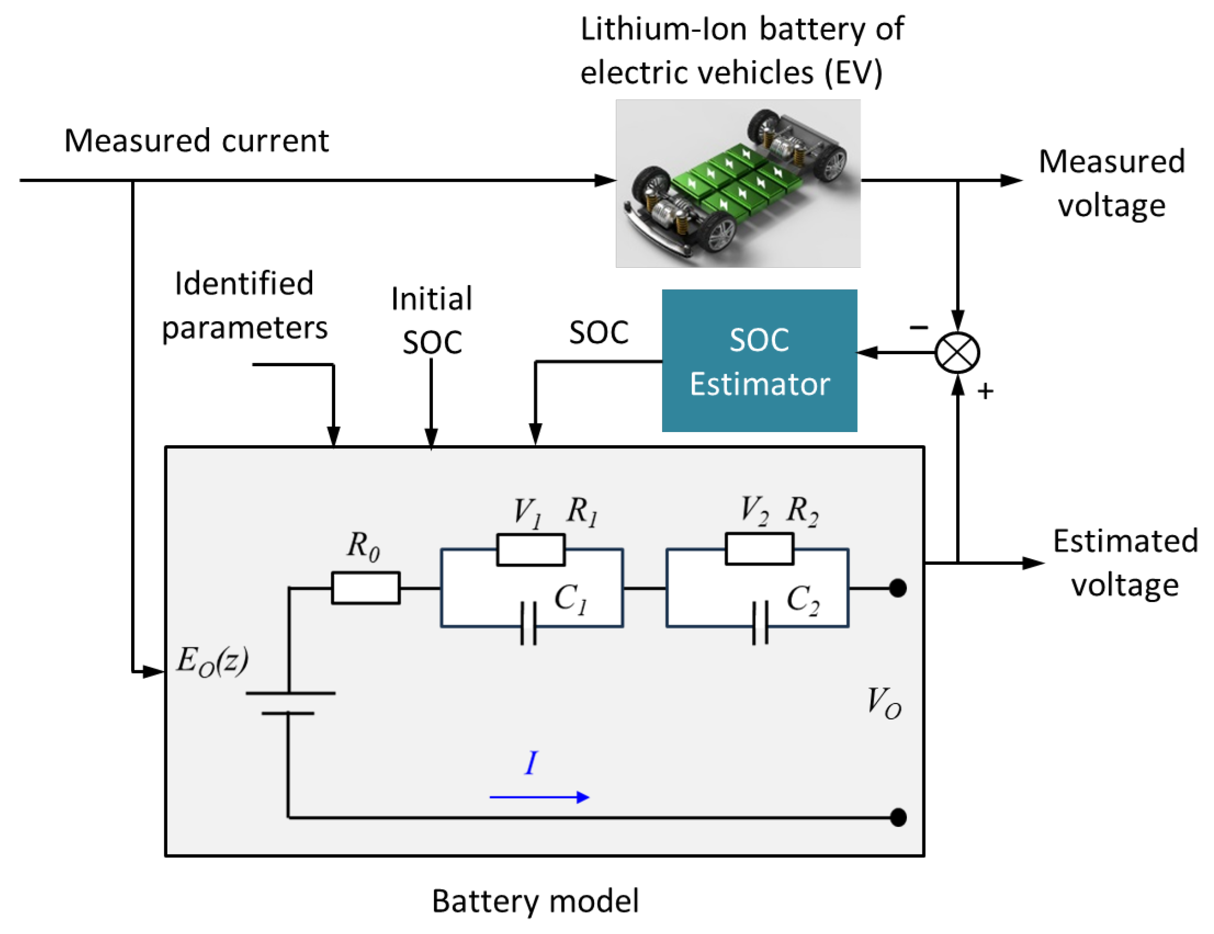
To reduce computational burden and improve SOC estimation accuracy, a multi-timescale framework was designed to co-estimate SOC and battery parameters because battery parameters are typically slowly changed, while battery states are rapidly changed. The discrete-time state-space equations are constructed via a multiscale approach, where the macro scale predicts the battery parameters in the system and the micro scale predicts the state of the system. The nonlinear state-space model of the system is then expressed as
{ x k , l + 1 = f ( x k , l , θ k , u k , l ) + ω k , l , θ k + 1 = θ k + ρ k y k , l = g ( x k , l , θ k , u k , l ) + ν k , l
where x k , l is the time t k , l = t k , 0 + l × T ( 1 l L ) system state matrix; T is a fixed time interval between two neighboring measurement points; k is a metric for the macroscale state; l is a metric for the microscale state; u k , l is the exogenous input matrix at moment t k , l ; y k , l is the system observation matrix; ω k , l and ρ k denote the state and process noise matrices, respectively; v k , l denotes the measurement noise matrix; θ k indicates the parameter matrix at the k th macroscale and θ k = θ k , 0 : L 1 . Note that L represents the level of separation on the timescale and x k = x k 1 , L . Our goal is to estimate the system state x and parameter θ from noisy observation y after defining the system.

2.1. Battery Model

The Thevenin ECM for the lithium-ion battery model is described in detail in [17]. To achieve a balance between the accuracy and complexity of the battery model, a second-order RC model was used to simulate battery dynamics in this study. The second-order RC is divided into five parts, including the open-circuit voltage E o ( z ) , ohmic resistor R 0 , resistor-capacitor network, terminal voltage V o , and operating current I. The symbols R 1 and R 2 in the resistor-capacitor network represent the polarization resistance; C 1 and C 2 represent the polarization capacitance; the corresponding V 1 and V 2 represent the voltages of these two networks. The battery was modeled according to Kirchhoff’s theorem, as shown in Equations (2) and (3):
State equation:
{ d V 1 d t = 1 R 1 C 1 V 1 + 1 C 1 I d V 2 d t = 1 R 2 C 2 V 2 + 1 C 2 I d S O C d t = 1 Q I ,
Output equation:
V o = E o ( S O C ) R 0 I V 1 V 2
where Q denotes the nominal capacity of the battery. SOC represents the ratio of the remaining capacity of the battery to its rated capacity, which is expressed using Equation (4) as
S O C t = S O C 0 1 Q 0 t I d t
where I and S O C t denote the current and the SOC at time t, respectively. From Equation (2), we can reformulate the following:
[ V k , l 1 V k , l 2 S O C k , l ] = [ 1 T s R 1 C 1 0 0 0 1 T s R 2 C 2 0 0 0 1 ] [ V k , l 1 1 V k , l 1 2 S O C k , l 1 ] + [ T s C 1 T s C 2 T s Q ] I k , l 1  
The state transition and measurement equations can be obtained using Equation (6).
{ x k , l + 1 = f ( x k , l , θ k , u k , l ) = [ 1 T s R 1 C 1 0 0 0 1 T s R 2 C 2 0 0 0 1 ] x k , l + [ T s C 1 T s C 2 T s Q ] u k , l y k , l = g ( x k , l , θ k , u k , l ) = E k , l o ( S O C ) R 0 u k , l V k , l 1 V k , l 2
where
{ x k , l = [ V k , l 1 V k , l 2 S O C k , l ] T θ k = [ R 0 R 1 R 2 C 1 C 2 Q ] k T y k , l = V k , l o u k , l = I k , l
where V k , l o and I k , l denote the battery voltage and current measured at time t k , l ; V k , l 1 and V k , l 2 represents the voltages of these two networks at time t k , l ; S O C k , l denotes the SOC at time t k , l . Furthermore, the C k θ calculation process requires the determination of the total derivative of the measurement function for the parameters. The computational procedure is described in detail in [21]. From Equation (6), the system state matrix and observation matrix are obtained as follows:
A k 1 , l 1 = [ 1 T s R 1 C 1 0 0 0 1 T s R 2 C 2 0 0 0 1 ] , B k 1 , l 1 = [ T s C 1 T s C 2 T s Q n ]
C k 1 , l x = [ 1 , 1 , E k 1 o ( S O C ) S O C k 1 , l ]
C k θ = [ i k , 0 0 0 0 0 E k 1 o ( S O C ) S O C k , 0 S O C k , 0 Q ^ k ] + C k , 0 x [ f ( x ^ k 1 , L 1 , θ ^ k , u k 1 , L 1 ) θ ^ k + f ( x ^ k 1 , L 1 , θ ^ k , u k 1 , L 1 ) x ^ k 1 , L 1 d x ^ k 1 , L 1 d θ ^ k ]

2.2. Online Parameter Identification of Battery Model

The parameters of the ECM are easily affected by factors such as the operating temperature, battery charge state, and aging degree; therefore, it is important to identify these parameters in real-time. To estimate the battery parameters, including R 0 , R 1 , R 2 , C 1 , C 2 , and Q, we adopted the EKF method [21] combined with online measurement data.

2.2.1. The Initial Values and Nonlinear Function

The hybrid pulse power characterization method was used to test the battery model parameters. One cycle of battery charging and discharging comprises three periods. During the charging period, the battery was first charged at a constant current of 0.5 C (1.5 A) until the voltage reached its cutoff voltage of 4.2 V, and then it was charged at a constant voltage of 4.2 V until the current reached its cutoff current of 0.05 C (0.15 A) to fill the battery. Subsequently, it was left for 2 h for the resting period. During the discharging period, the battery was discharged at a constant current of 1 C (3 A), left to rest for 2 h, and then discharged again at the equivalent current. Each time the SOC decreased by 5% until it was fully discharged. The initial values of these parameters are listed in Table 1. These initial values were obtained by parameter identification of the instantaneous voltage waveforms recorded in real-time using the least squares method [18]. The relationship between the OCV and SOC was obtained from the voltage waveforms of the pulse-discharge experiment. A seventh-order polynomial was used to accurately fit the measured data, as shown in Equation (11).
E O ( S O C ) = 76.8489 S O C 7 273.2551 S O C 6 + 389.1130 S O C 5 286.6882 S O C 4 + 119.2722 S O C 3 29.5698 S O C 2 + 5.5458 S O C + 2.8792

2.2.2. EKF-Based Online Parameter Estimation

The EKF provides an efficient approximation of likelihood estimation for nonlinear state discretization. A multiscale dual EKF was used for the macroscopic and microscopic prediction of system parameters and system states, respectively [21]. This approach reduces the computational cost of the BMS. Unlike the multiscale dual EKF, we use a single EKF with the designed MIARUKF algorithm to make macroscopic and microscopic predictions of the system parameters and system state, respectively. This co-estimation algorithm EKF-MIARUKF is multiscale and presented in Table 2. Steps 1 and 5 estimate the parameters using the EKF algorithm, and steps 2–4 estimate the SOC using the MIARUKF algorithm, as described in Section 3. From Table 2, θ 0 and P 0 θ are the initial values of the parameters and parameter covariance, respectively; x 0 , 0 and P 0 , 0 x are the initial values of the system state and covariance, respectively; Q 0 θ and R 0 θ are the initial values of the covariance of the parameter-estimated process noise and measurement noise, respectively; Q 0 , 0 x and R 0 , 0 x are the initial values of the covariance of the SOC-estimated process noise and measurement noise, respectively; K k θ is the Kalman gain of the parameter.
Table 2. Co-estimation algorithm EKF-MIARUKF.
Initialization(12)
θ 0 = E ( θ 0 ) , P 0 θ = E [ ( θ 0 θ ^ 0 ) ( θ 0 θ ^ 0 ) T ] , x 0 , 0 = E [ x 0 , 0 ] , P 0 , 0 x = E [ ( x 0 , 0 x ^ 0 , 0 ) ( x 0 , 0 x ^ 0 , 0 ) T ] Q 0 θ = E [ ( ρ 0 ρ ^ 0 ) ( ρ 0 ρ ^ 0 ) T ] , Q 0 , 0 x = E [ ( ω 0 , 0 ω ^ 0 , 0 ) ( ω 0 , 0 ω ^ 0 , 0 ) T ] R 0 θ = E [ ( ν 0 ν ^ 0 ) ( ν 0 ν ^ 0 ) T ] , R 0 , 0 x = E [ ( ν 0 , 0 ν ^ 0 , 0 ) ( ν 0 , 0 ν ^ 0 , 0 ) T ]
For k { 1 , , } , calculation:
Step 1 Macroscale EKF parameter filter θ ^ k time update equation
(13)
θ ^ k = θ ^ k 1 , P k θ = P k 1 θ + Q k 1 θ
For k { 1 , , } , compute state filters at each micro scale
Step 2 Microscale MIARUKF filter state time and measurement update equations
Equations (17)–(33)
Step 3 For time-series calculation l = 1 : L ( l L ) , L is set to 60 s
Equations (17)–(33)
Step 4 Timescale transform(14)
x ^ k , 0 = x ^ k 1 , L , P k , 0 x = P k 1 , L x , y k , 0 = y k 1 , L , u k , 0 = u k 1 , L
For k { 1 , , } , calculation:
Step 5 Macroscale EKF parametric filter θ ^ k update equation
(15)
K k θ = P k θ ( C k θ ) T [ C k θ P k θ ( C k θ ) T + R k θ ] θ ^ k = θ ^ k + K k θ [ y k , 0 g ( x ^ k , 0 , θ ^ k , u k , 0 ) ] P k θ = ( I K k θ C k θ ) P k θ
where     C k 1 , l x = g ( x , θ ^ k , u k 1 , l ) x | x = x ^ k 1 , l ,   C k θ = d g ( x ^ k , 0 , θ , u k , 0 ) d θ | θ = θ ^ k (16)

3. SOC Estimation

3.1. Overview

In this study, we combined the ARUKF with multi-innovation based on the principle of multi-innovation, which is MIARUKF, where the ARUKF is the combination of a robust unscented Kalman filter (RUKF) [28] and the adaptation process in the adaptive extended Kalman filtering [29]. However, a multi-innovation iterative process contains multiple steps of prediction information, resulting in the possibility that the accumulation of old data interferes with the results when there is a measurement error [30]. To overcome this problem, Liu et al. [31] proposed a multi-innovation adaptive extended Kalman filtering to regulate the correction effect of old data by adding different weighting factors to different innovations. The MIARUKF algorithm is summarized as follows:
Obtain Sigma point at time step k − 1, l − 1:
{ x k 1 , l 1 0 = x ^ k 1 , l 1 x k 1 , l 1 i = x ^ k 1 , l 1 + ( n + λ ) P k 1 , l 1 x , i = 1 , 2 , , n x k 1 , l 1 i = x ^ k 1 , l 1 ( n + λ ) P k 1 , l 1 x , i = n + 1 , n + 2 , , 2 n
where n denotes the length of the state vector and λ can be calculated as
λ = α 2 ( n + h ) n ,
where α is the scale parameter, α [ 0,1 ] is used to control the distribution of sigma points, and h is also a scale parameter. In this paper, the α is 0.01, and h is 0. The weights of the mean and covariance are calculated as follows:
{ W m 0 = λ n + λ , W m i = 1 2 ( n + λ ) , i = 1 , 2 2 n W c 0 = λ n + λ + 1 α 2 + β , W c i = 1 2 ( n + λ ) , i = 1 , 2 2 n
  • where W m and W c represent the weights for calculating the mean and covariance, respectively, and β 0 is a nonnegative term, and, in this study, the Gaussian random variable β is set to 2.
  • Update the a priori state value x ^ k 1 , l and the system variance prediction P k 1 , l x x :
    x ^ k 1 , l = i = 0 2 n W m i x k 1 , l 1 i P k 1 , l x x = i = 0 2 n W c i ( x k 1 , l 1 i x ^ k 1 , l ) ( x k 1 , l 1 i x ^ k 1 , l ) T + Q k 1 , l 1 x
    where Q k 1 , l 1 x represents the system noise covariance matrix.
  • Update observation y ^ k 1 , l and observation variance prediction P k 1 , l y y :
    y ^ k 1 , l = i = 0 2 n W m i y k 1 , l 1 i P k 1 , l y y = i = 0 2 n W c i ( y k 1 , l 1 i y ^ k 1 , l ) ( y k 1 , l 1 i y ^ k 1 , l ) T + R k 1 , l 1 x
    where R k 1 , l 1 x represents the process noise covariance matrix.
  • Update covariance P k 1 , l x y , Kalman gain K k 1 , l x and state error covariance P k 1 , l x :
    P k 1 , l x y = i = 0 2 n W c i ( x k 1 , l 1 i x ^ k 1 , l ) ( y k 1 , l 1 i y ^ k 1 , l ) T K k 1 , l x = P k 1 , l x y ( P k 1 , l x y ) 1 P k 1 , l x = P k 1 , l x x [ P k 1 , l x y P k 1 , l x x ] ( R ) 1 [ P k 1 , l x y P k 1 , l x x ] T
    where
    R = [ R k 1 , l 1 x 0 0 γ I ] + [ H k , l 1 I ] P K [ H k , l 1 T I ] = [ R k 1 , l 1 x + P k 1 , l y y ( P k 1 , l x y ) T P k 1 , l x y γ 2 I + P k 1 , l x x ] ,
Selection factor γ is set to 3, and I is the unit matrix.
  • Multi-Innovation Status Measurement Update:
    x ^ k 1 , l = x ^ k 1 , l + i = 1 b λ i K k , l i e k , l i + 1 ,
    where b denotes the length of the innovation. The weights at different moments are represented by Equation (25), which ensures the maximum weight at the current moment.
    λ 1 ( λ 2 + λ 3 + λ b )
The effect of the cumulative interference was reduced by adding different weighting factors to the gain at different time intervals to play the role of correcting the old data. The performance of MIARUKF is at least better than that of ARUKF with different weights, as follows:
{ λ 1 = 1 λ 2 = λ 3 = λ b = a b 1 , 0 a 1
where the adjustable coefficient a is 0.9.
Although good algorithmic results can be obtained by adding an appropriate number of multiple innovations to the MIARUKF, the performance of the algorithm deteriorates when too many innovations are incorporated. To ensure the excellent performance of MIARUKF, the innovation length must be constrained.
  • Update adaptive process noise covariance matrix Q ^ k 1 , l x and measurement noise covariance matrix R ^ k 1 , l x :
    Q ^ k 1 , l x = K k 1 , l x N ^ ( d k 1 , l ) K k 1 , l x T
    R ^ k 1 , l x = N ^ ( e k 1 , l ) + C k 1 , l x P k 1 , l x C k 1 , l x T
Innovation at moment t k 1 , l is d k 1 , l , which is the difference between the actual observation y k 1 , l and predicted observation y ^ k 1 , l d :
d k 1 , l = y k 1 , l y ^ k 1 , l d
where
y ^ k 1 , l d = y ^ k 1 , l
The residual at moment t k 1 , l is e k 1 , l , which is the difference between the actual observation y k 1 , l and estimated observation y ^ k 1 , l e :
e k 1 , l = y k 1 , l y ^ k 1 , l e
where
y ^ k 1 , l e = [ 1 1 0 ] x ^ k 1 , l + R 0 u k 1 , l + E k , l o ( S O C )
Assuming that d k 1 , l is ergodic, the real-time estimated variance of innovation can be obtained based on the windowing method as (33):
N ^ ( d k 1 , l ) = { l 1 l N ^ ( d k 1 , l 1 ) + 1 l d k 1 , l d k 1 , l T l W 1 W i = l W + 1 l d i d i T l > W
where W denotes the length of the sliding data window.

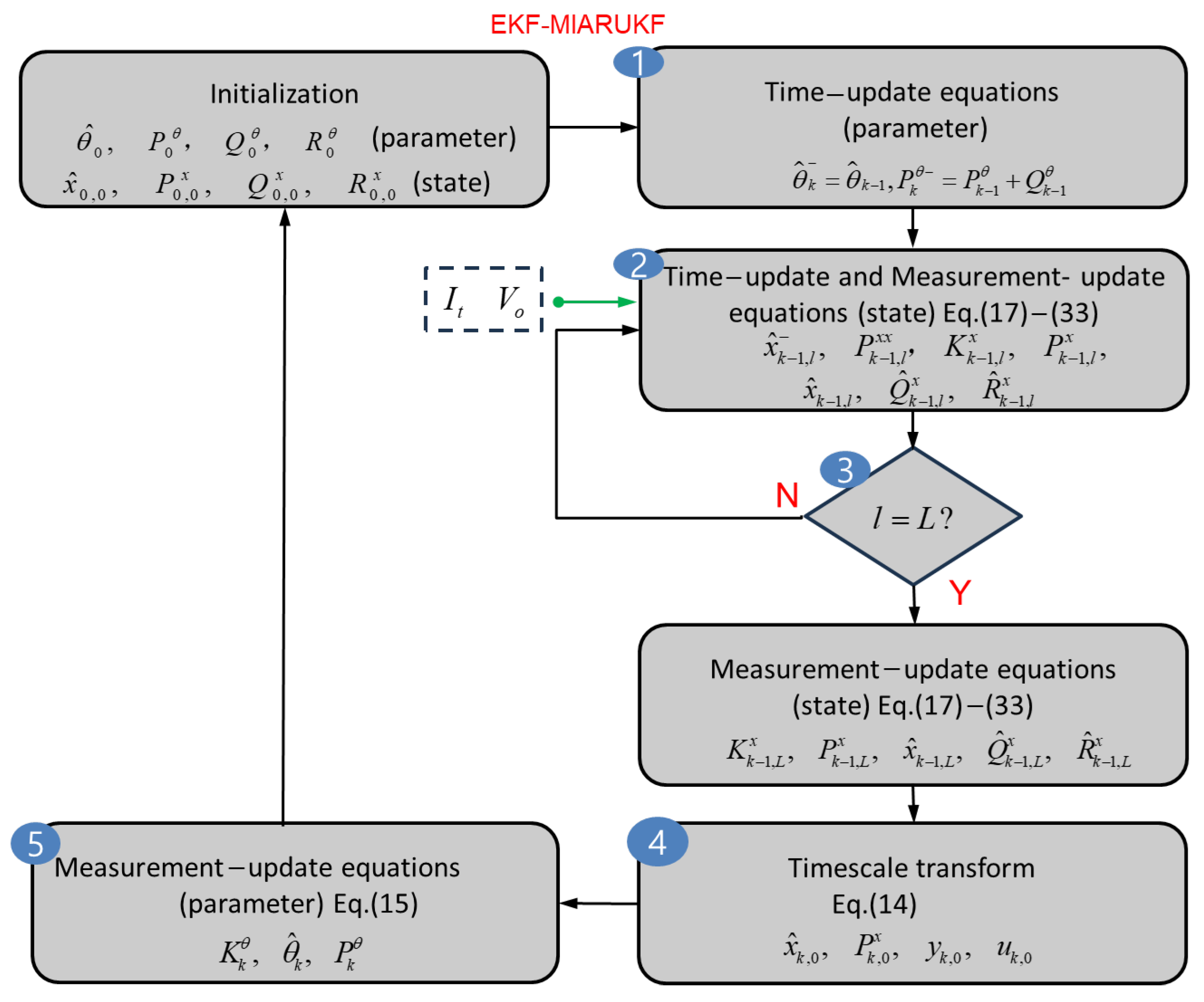
3.2. Implementation of the Co-Estimation Algorithm

The multiscale co-estimation algorithm EKF-MIARUKF uses a five-step estimation, as shown in Figure 2.
  • At each macroscale level, the EKF performs a temporal update and computes a priori parameter estimates θ ^ k and error covariances P k θ using Equation (13). The battery capacity was updated along with the battery model parameters.
  • After the temporal update of the macroscopic EKF, state estimation and measurement updates of the microscopic MIARUKF were performed at each microscale using θ ^ k . The a priori state estimation x ^ k 1 , l and its error covariance P k 1 , l x x , the a posteriori state estimation x ^ k 1 , l and its error covariance P k 1 , l x , the adaptive process noise covariance Q ^ k 1 , l x , and the adaptive measurement noise covariance R ^ k 1 , l x were computed from Equations (17)–(33).
  • After a posteriori estimation was completed, we compared the microscale l and timescale separation level L. If microscale l does not reach L, the state estimate x ^ k 1 , l is passed to step 2 and used as the initial value at time t k 1 , L before the state estimation is performed. If l reaches L, the a posteriori state estimate x ^ k 1 , L and its error covariance P k 1 , L x , adaptive process noise covariance Q ^ k 1 , L x , and adaptive measurement noise covariance R ^ k 1 , L x can be updated using Equations (17)–(33) for the next macro time.
  • Update all microscopic timescales according to Equation (14); for example, x ^ k 1 , L = x ^ k , 0 . In simpler terms, the estimates at t k 1 , L are ready to be updated for parameter and next-state estimations.
  • After state estimation, the macroscopic EKF performs measurement updating, where the posterior estimate θ ^ k and covariance P k θ are computed from Equation (15).

4. Experimental Validation and Discussion

An experimental prototype testbed was established to experimentally validate the proposed co-estimation algorithm. Based on a high-precision test platform, a compact-size lithium-ion battery [32] (model: 18650-30Q) was used for the initial experiment. Its nominal voltage was 4.2 V, and its nominal capacity was 3 Ah. A single-cell battery was used as a testbed. The experimental set-up comprises a temperature chamber, computer, and battery test system (BTS-4000) for current (0–6 A) and voltage (0–5 V). The voltage and current errors were limited to 0.1%. Experimental data, including charging and discharging currents, as well as output voltages, were collected and stored at 0.1 s intervals by a computer connected to the BTS-4000. The process of data acquisition was: first, the battery was placed in a temperature chamber (25 °C) and connected; then the battery was fully charged and left to stand for two hours using the constant current and constant voltage mode through the host computer; then the dynamic condition file was imported through the host computer and the protection voltage was set to 2.5 V; and finally the charging and discharging battery device was run; at the end of the experiment the data was imported to the computer connected to the host computer. Note that the experiments were performed under fully charged conditions, and the designed SOC estimation method was evaluated based on the experimental data of different operating conditions. A block diagram of the experimental bench is shown in Figure 3.

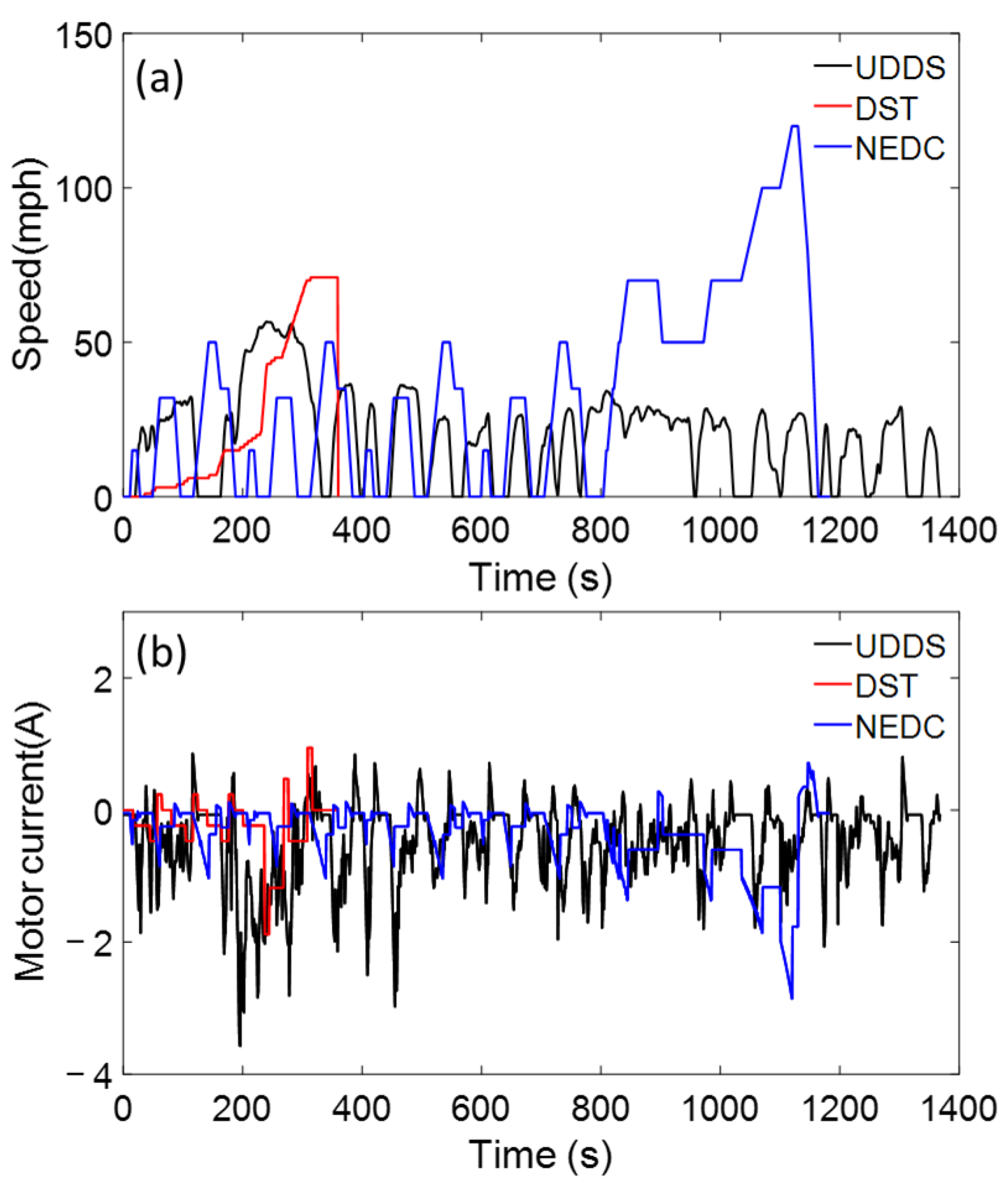
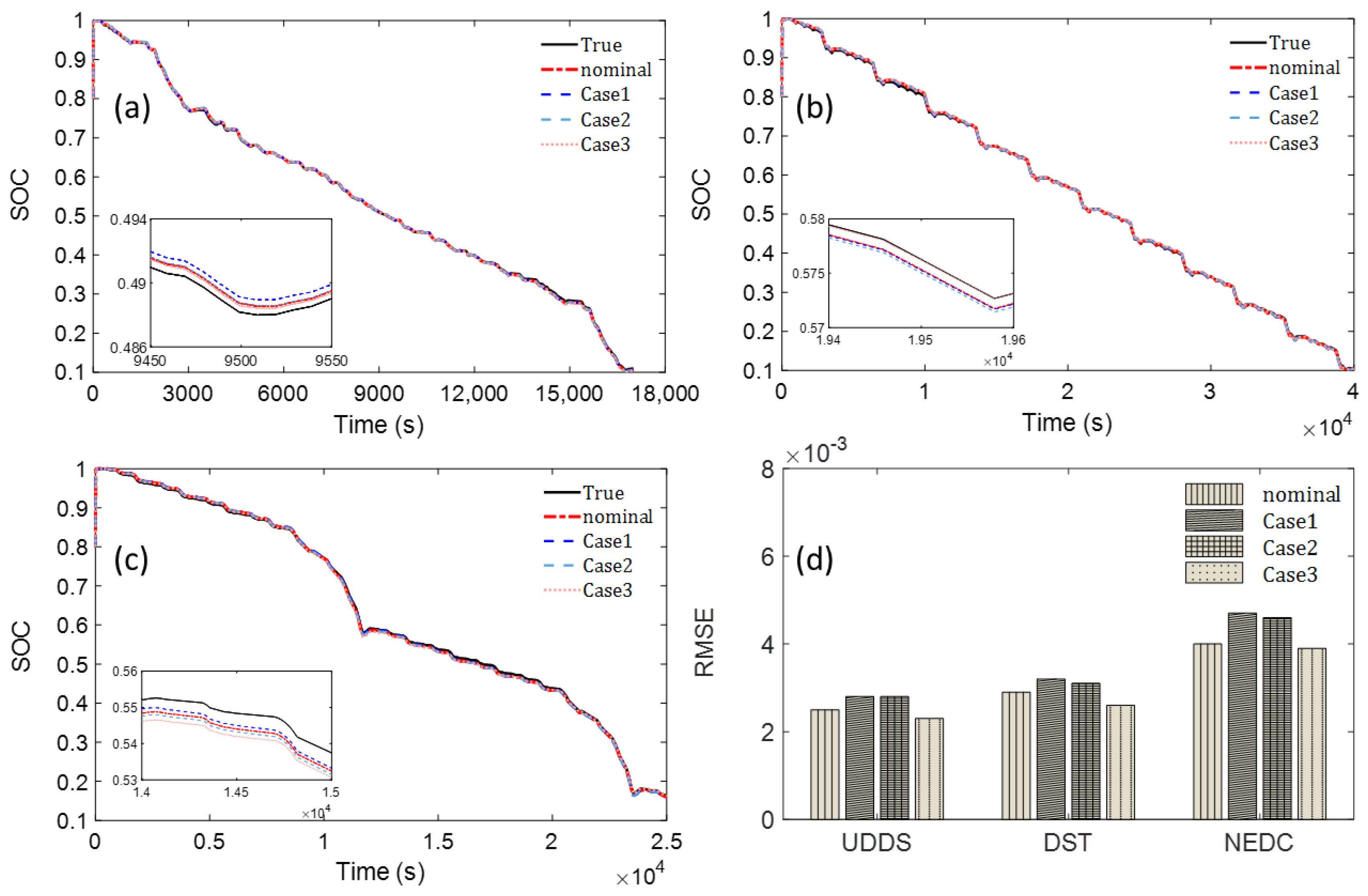
4.1. Dynamic Condition Testing

To evaluate the performance of the proposed algorithm under various dynamic driving conditions, an SOC estimation experiment was performed under driving cycles. Because the inadequate representativeness of driving cycles is one significant factor leading to the discrepancy, three driving cycles, UDDS, DST, and NEDC, were used to represent the real-world driving conditions and were widely used in the automotive industry to evaluate the performance associated with vehicle’s dynamic conditions. The single-cycle speed profiles for the three driving cycles are shown in Figure 4a. We used a simulation software (Version: ADVISOR 2003) to generate three corresponding motor current curves based on this criterion, as shown in Figure 4b. Note that our motor current curves are the result of equal scaling down based on the current that the battery can provide because the power source in this experiment is a single lithium-ion battery, which is unable to provide the current output (i.e., electrical load) under real working conditions. The battery test equipment controls the battery through a single-cycle condition file to carry out multiple cycles of charging and discharging and stops working when the battery capacity drops from full capacity to the cut-off voltage. Figure 5, Figure 6 and Figure 7 present the results of online identification of the model parameters under these three working conditions. The trends in the parameter identification results under different working conditions appear to be similar. In addition, the small fluctuations in the early stage parameters R 0 , R 1 , R 2 , C 1 , C 2 , and Q are owing to the use of hybrid pulse power characterization experiments to determine the initial values of the model parameters.
The SOC under various cycles was estimated based on the identified model parameters. In this study, the designed EKF-MIARUKF algorithm was compared with the SOC estimation results of the MIARUKF, ARUKF, and RUKF algorithms, as shown in Figure 8a–c. Notably, algorithms MIARUKF, ARUKF, and RUKF use fixed parameter values computed in advance. For a more comprehensive comparison of the estimation accuracy of the different algorithms, we calculated the RMSE between the estimated and true SOC. RMSE is shown by Equation (34). To further demonstrate the advantages of the proposed algorithm, we calculated the MAE between the estimated SOC and the true SOC. The MAE is shown in Equation (35).
R M S E ( k ) = 1 k i = 1 k ( x ( i ) x ^ ( i ) ) 2
M A E ( k ) = i = 1 k | x ( i ) x ^ ( i ) | k
where k, x ( i ) , and x ^ ( i ) represent the time instant, true SOC, and estimated SOC, respectively. The RMSE results are presented in Figure 8d. The MAE for different algorithms are compared and summarized in Table 3. By comparing the SOC estimates with the true values, it is evident that the designed EKF-MIARUKF algorithm estimates the SOC more accurately than the other current algorithms. Therefore, the adaptive algorithm shows better SOC estimation performance than the non-adaptive algorithm.

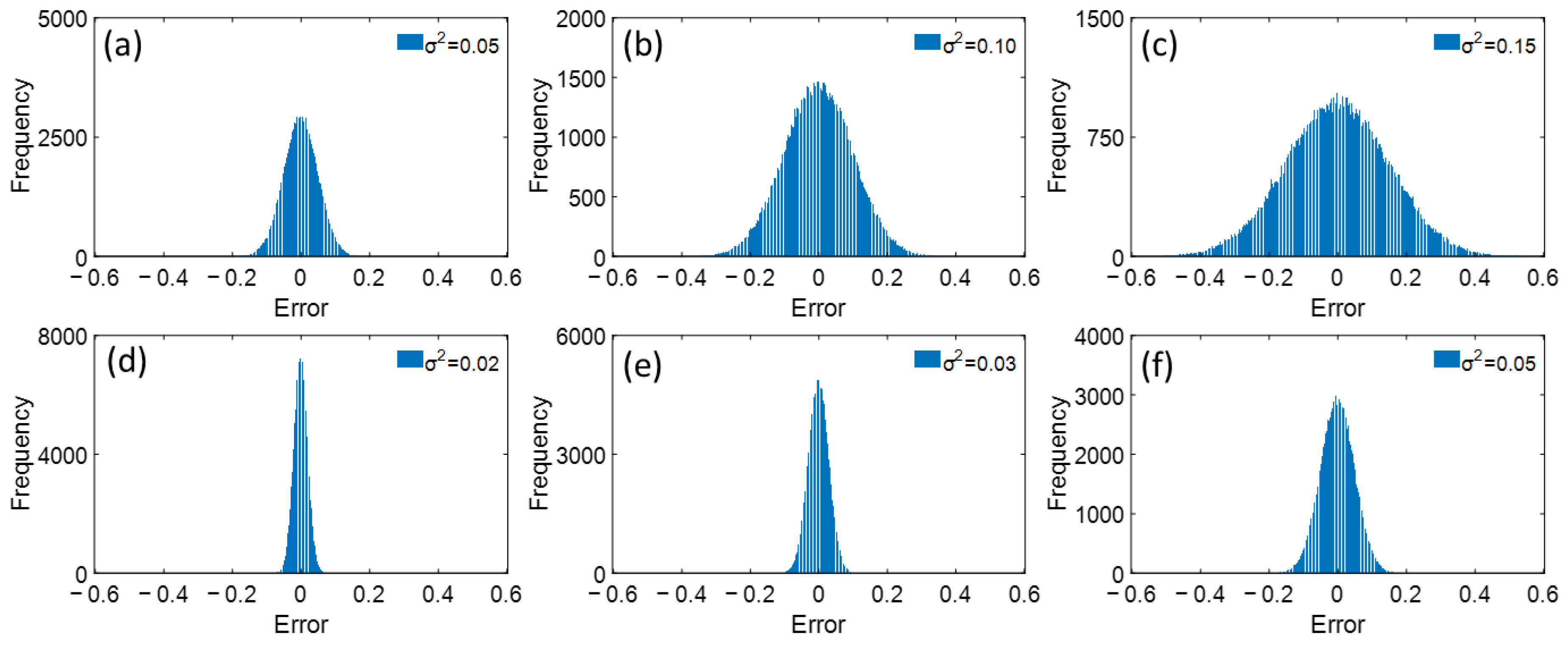
4.2. Robustness Analysis

In practical applications, the sensor information in automobiles is contaminated by electrical noise. Therefore, we examine the effect of electrical noise (i.e., different variances) on the performance of SOC estimation algorithms. This is confirmed by adding random Gaussian white noise to the measured current and voltage data. The white Gaussian random noise used here was categorized into three cases—case 1, case 2, and case 3—with contamination levels ranging from low to high. The measured current and voltage data of case 1 are added with Gaussian white noise in Figure 9a (σ2 = 0.05) and (d) (σ2 = 0.02), the measured current and voltage data of case 2 are added with Gaussian white noise in Figure 9b (σ2 = 0.10) and (e) (σ2 = 0.03), and the measured current and voltage data of case 3 are added with Gaussian white noise in Figure 9c (σ2 = 0.15) and (f) (σ2 = 0.05), respectively. As shown in Figure 10a,d, after adding different noises to the experimental data under the UDDS cycle, the EKF-MIARUKF algorithm still maintains a high estimation accuracy, with a small change in the value of mean root mean square error (MRMSE).
The identical noise was added for the DST and NEDC cycles. As shown in Figure 10b–d, the SOC estimation results of the algorithm show little fluctuation, and the RMSE results are similar when subjected to noise interference under different dynamic conditions. To further investigate the performance with the addition of noise, the relative error of the nominal MRMSE (i.e., the normalized performance measure) was calculated quantitatively as follows:
Relative   Error = M R M S E Perturbed M R M S E Nominal M R M S E Nominal
The relative errors of the estimated and nominal values for the three cases are listed in Table 4, Table 5, and Table 6, respectively. The results show that the estimated performance and nominal values are similar for the different cases.

5. Conclusions

In this study, a co-estimation method EKF-MIARUKF for parameter and SOC estimation based on multiple timescales was successfully developed. The second-order Thevenin ECM method was utilized to characterize the externals of the LIB, and the EKF was employed to estimate various parameters of the ECM online and thus the influence of fixed parameters on the SOC estimation results. The designed MIARUKF algorithm is a reliable SOC estimator that not only adjusts the noise covariance to improve adaptability but also incorporates a weighting factor in each innovation point based on the multi-innovation principle to minimize the cumulative effect of historical disturbances. Coordinating the time variation of the EKF and MIARUKF through the multi-timescale framework reduces the computational effort while obtaining accurate parameters. To validate the proposed multi-timescale EKF-MIARUKF method, experiments with various automotive operating conditions were conducted and the SOC prediction accuracy of different algorithms was judged by RMSE and MAE. The SOC estimation accuracy of the designed algorithm was higher than other algorithms. The robustness of the algorithm was evaluated by adding current and voltage noise to the experimental data. The results show that the EKF-MIARUKF algorithm is robust to interference. This research contributes to the development of an EV BMS system that improves the efficiency of energy use through accurate SOC estimation, which in turn improves EV range and battery lifespan. At the same time, the development of this technology will not only improve the performance of EVs themselves but also reduce carbon emissions and promote the development of renewable energy.
Notably, the temperature inside and around the battery in a real driving environment varies, but the experiments in this work were conducted at a constant room temperature (25 °C), ignoring the effects of other temperatures. Moreover, the battery has a lifetime, and the battery capacity will decrease after the battery undergoes multiple charging and discharging; the battery aging tests and the estimation of the results after battery aging were not performed in this work. Future research will focus on two issues: (1) the accuracy of the algorithm estimation at other temperatures and (2) the accuracy of the algorithm estimation after battery aging. Accordingly, three plans are proposed to address these two issues: (1) to conduct experiments in low and high-temperature environments; (2) to conduct experiments in environments with a certain range of temperature variations; and (3) to conduct battery aging tests.

Author Contributions

G.-W.K. as the principal investigator takes the primary responsibility for this research. C.L. performed the experiments and analyzed. All authors have read and agreed to the published version of the manuscript.

Funding

This work was supported by an INHA UNIVERSITY Research Grant.

Data Availability Statement

The datasets used and/or analyzed during the current study are available from the corresponding author upon reasonable request.

Acknowledgments

The authors thank the Core Facility Center for Sustainable Energy (Inha University) for providing the measurement instruments.

Conflicts of Interest

The authors declare no conflict of interest.

References

  1. Hu, X.; Yuan, H.; Zou, C.; Li, Z.; Zhang, L. Co-estimation of state of charge and state of health for lithium-ion batteries based on fractional-order calculus. IEEE Trans. Veh. Technol. 2018, 67, 10319–10329. [Google Scholar] [CrossRef]
  2. Takami, N.; Inagaki, H.; Tatebayashi, Y.; Saruwatari, H.; Honda, K.; Egusa, S. High-power and long-life lithium-ion batteries using lithium titanium oxide anode for automotive and stationary power applications. J. Power Sources 2013, 244, 469–475. [Google Scholar] [CrossRef]
  3. Hoque, M.; Hannan, M.; Mohamed, A.; Ayob, A. Battery charge equalization controller in electric vehicle applications: A review. Renew. Sustain. Energy Rev. 2017, 75, 1363–1385. [Google Scholar] [CrossRef]
  4. Cheng, K.W.E.; Divakar, B.; Wu, H.; Ding, K.; Ho, H.F. Battery-management system (BMS) and SOC development for electrical vehicles. IEEE Trans. Veh. Technol. 2010, 60, 76–88. [Google Scholar] [CrossRef]
  5. Waag, W.; Fleischer, C.; Sauer, D.U. Critical review of the methods for monitoring of lithium-ion batteries in electric and hybrid vehicles. J. Power Sources 2014, 258, 321–339. [Google Scholar] [CrossRef]
  6. Ng, K.S.; Moo, C.-S.; Chen, Y.-P.; Hsieh, Y.-C. Enhanced coulomb counting method for estimating state-of-charge and state-of-health of lithium-ion batteries. Appl. Energy 2009, 86, 1506–1511. [Google Scholar] [CrossRef]
  7. Xing, Y.; He, W.; Pecht, M.; Tsui, K.L. State of charge estimation of lithium-ion batteries using the open-circuit voltage at various ambient temperatures. Appl. Energy 2014, 113, 106–115. [Google Scholar] [CrossRef]
  8. Yang, N.; Zhang, X.; Li, G. State of charge estimation for pulse discharge of a LiFePO4 battery by a revised Ah counting. Electrochim. Acta 2015, 151, 63–71. [Google Scholar] [CrossRef]
  9. Chemali, E.; Kollmeyer, P.J.; Preindl, M.; Emadi, A. State-of-charge estimation of Li-ion batteries using deep neural networks: A machine learning approach. J. Power Sources 2018, 400, 242–255. [Google Scholar] [CrossRef]
  10. How, D.N.; Hannan, M.A.; Lipu, M.S.H.; Sahari, K.S.; Ker, P.J.; Muttaqi, K.M. State-of-charge estimation of li-ion battery in electric vehicles: A deep neural network approach. IEEE Trans. Ind. Appl. 2020, 56, 5565–5574. [Google Scholar] [CrossRef]
  11. Chen, C.; Xiong, R.; Yang, R.; Shen, W.; Sun, F. State-of-charge estimation of lithium-ion battery using an improved neural network model and extended Kalman filter. J. Clean. Prod. 2019, 234, 1153–1164. [Google Scholar] [CrossRef]
  12. Hannan, M.A.; Lipu, M.S.H.; Hussain, A.; Saad, M.H.; Ayob, A. Neural network approach for estimating state of charge of lithium-ion battery using backtracking search algorithm. IEEE Access 2018, 6, 10069–10079. [Google Scholar] [CrossRef]
  13. Anton, J.C.A.; Nieto, P.J.G.; Viejo, C.B.; Vilán, J.A.V. Support vector machines used to estimate the battery state of charge. IEEE Trans. Power Electron. 2013, 28, 5919–5926. [Google Scholar] [CrossRef]
  14. Wang, Y.; Yang, D.; Zhang, X.; Chen, Z. Probability based remaining capacity estimation using data-driven and neural network model. J. Power Sources 2016, 315, 199–208. [Google Scholar] [CrossRef]
  15. Zhang, Q.; Wang, D.; Yang, B.; Cui, X.; Li, X. Electrochemical model of lithium-ion battery for wide frequency range applications. Electrochim. Acta 2020, 343, 136094. [Google Scholar] [CrossRef]
  16. Nejad, S.; Gladwin, D.; Stone, D. A systematic review of lumped-parameter equivalent circuit models for real-time estimation of lithium-ion battery states. J. Power Sources 2016, 316, 183–196. [Google Scholar] [CrossRef]
  17. Plett, G.L. Battery Management Systems, Volume I: Battery Modeling; Artech House: Norwood, MA, USA, 2015. [Google Scholar]
  18. Zhu, Q.; Xiong, N.; Yang, M.-L.; Huang, R.-S.; Hu, G.-D. State of charge estimation for lithium-ion battery based on nonlinear observer: An H∞ method. Energies 2017, 10, 679. [Google Scholar] [CrossRef]
  19. Yang, H.; Sun, X.; An, Y.; Zhang, X.; Wei, T.; Ma, Y. Online parameters identification and state of charge estimation for lithium-ion capacitor based on improved Cubature Kalman filter. J. Energy Storage 2019, 24, 100810. [Google Scholar] [CrossRef]
  20. Li, X.; Wang, Z.; Zhang, L. Co-estimation of capacity and state-of-charge for lithium-ion batteries in electric vehicles. Energy 2019, 174, 33–44. [Google Scholar] [CrossRef]
  21. Xiong, R.; Sun, F.; Chen, Z.; He, H. A data-driven multi-scale extended Kalman filtering based parameter and state estimation approach of lithium-ion polymer battery in electric vehicles. Appl. Energy 2014, 113, 463–476. [Google Scholar] [CrossRef]
  22. Guo, F.; Hu, G.; Xiang, S.; Zhou, P.; Hong, R.; Xiong, N. A multi-scale parameter adaptive method for state of charge and parameter estimation of lithium-ion batteries using dual Kalman filters. Energy 2019, 178, 79–88. [Google Scholar] [CrossRef]
  23. Panda, S.; Tripura, T.; Hazra, B. First-order error-adapted eigen perturbation for real-time modal identification of vibrating structures. J. Vib. Acoust. 2021, 143, 051001. [Google Scholar] [CrossRef]
  24. Bhowmik, B.; Tripura, T.; Hazra, B.; Pakrashi, V. Real time structural modal identification using recursive canonical correlation analysis and application towards online structural damage detection. J. Sound Vib. 2020, 468, 115101. [Google Scholar] [CrossRef]
  25. Bhowmik, B.; Tripura, T.; Hazra, B.; Pakrashi, V. First-order eigen-perturbation techniques for real-time damage detection of vibrating systems: Theory and applications. Appl. Mech. Rev. 2019, 71, 060801. [Google Scholar] [CrossRef]
  26. Sun, F.; Hu, X.; Zou, Y.; Li, S. Adaptive unscented Kalman filtering for state of charge estimation of a lithium-ion battery for electric vehicles. Energy 2011, 36, 3531–3540. [Google Scholar] [CrossRef]
  27. Zhang, S.; Guo, X.; Zhang, X. An improved adaptive unscented Kalman filtering for state of charge online estimation of lithium-ion battery. J. Energy Storage 2020, 32, 101980. [Google Scholar] [CrossRef]
  28. Havangi, R. Adaptive robust unscented Kalman filter with recursive least square for state of charge estimation of batteries. Electr. Eng. 2022, 104, 1001–1017. [Google Scholar] [CrossRef]
  29. Liu, Y.; Huangfu, Y.; Xu, J.; Zhao, D.; Xu, L.; Xie, M. State-of-charge co-estimation of Li-ion battery based on on-line adaptive extended Kalman filter carrier tracking algorithm. In Proceedings of the IEEE Industrial Electronics Society, 44nd Annual Conference (IECON 2018), Washington, DC, USA, 21–23 October 2018; pp. 1940–1945. [Google Scholar]
  30. Xie, S.; Chen, D.; Chu, X.; Liu, C. Identification of ship response model based on improved multi-innovation extended Kalman filter. J. Harbin Eng. Univ. 2018, 39, 282–289. [Google Scholar]
  31. Liu, Z.; Dang, X.; Jing, B. A novel open circuit voltage based state of charge estimation for lithium-ion battery by multi-innovation Kalman filter. IEEE Access 2019, 7, 49432–49447. [Google Scholar] [CrossRef]
  32. Panchal, S.; Mathew, M.; Fraser, R.; Fowler, M. Electrochemical thermal modeling and experimental measurements of 18650 cylindrical lithium-ion battery during discharge cycle for an EV. Appl. Therm. Eng. 2018, 135, 123–132. [Google Scholar] [CrossRef]
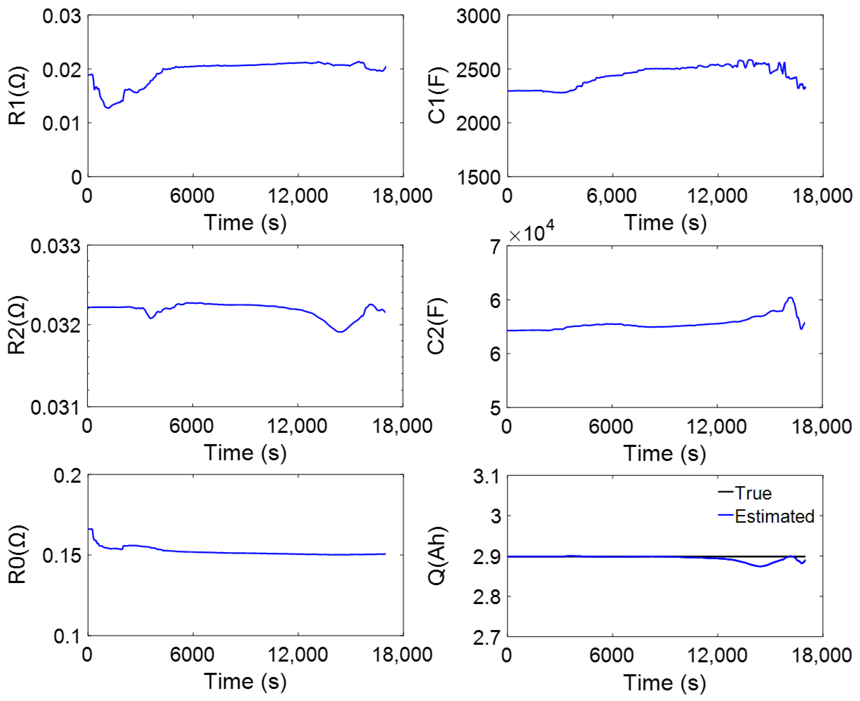
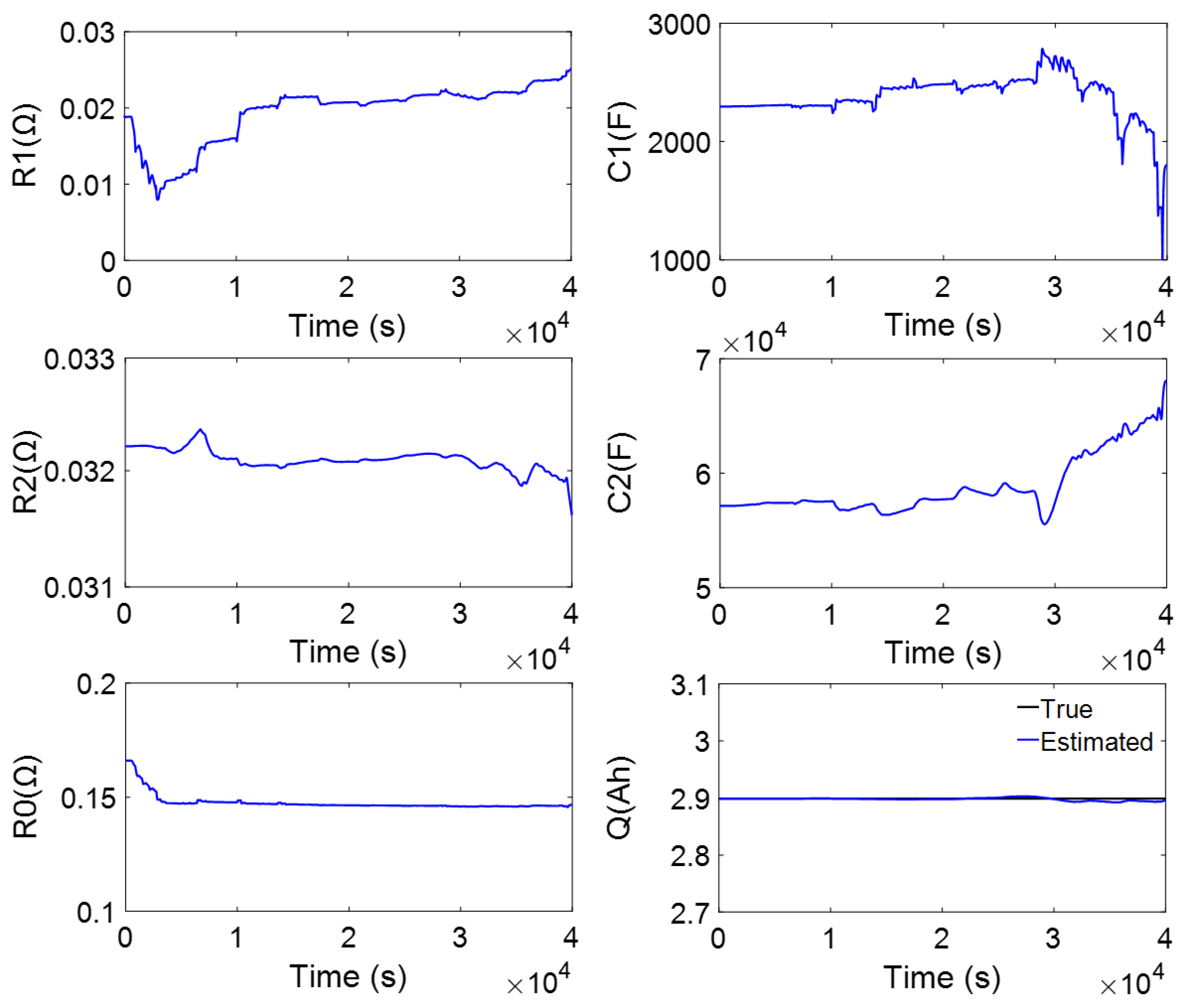
Figure 1. Block diagram of the model-based SOC estimation algorithm.
Energies 17 00272 g001
Figure 2. Implementation of the proposed co-estimation algorithm.
Energies 17 00272 g002
Figure 3. Experimental set-up for estimating SOC of lithium-ion batteries.
Energies 17 00272 g003
Figure 4. UDDS, DST, and NEDC drive cycles: (a) speed profile, (b) motor current profile.
Energies 17 00272 g004
Figure 5. Parameter identification of R 0 , R 1 , R 2 , C 1 , C 2 and Q under the UDDS cycle.
Energies 17 00272 g005
Figure 6. Parameter identification of R 0 , R 2 , C 1 , C 2 , and Q under the DST cycle.
Energies 17 00272 g006
Figure 7. Parameter identification of R 0 , R 1 , R 2 , C 1 , C 2 , and Q under the NEDC cycle.
Energies 17 00272 g007
Figure 8. Comparison of SOC estimation under dynamic conditions: (a) under the UDDS cycle, (b) under the DST cycle, (c) under the NEDC cycle, (d) RMSE.
Energies 17 00272 g008
Figure 9. Gaussian random noises for robustness evaluation under the UDDS cycle: (a,d) less contaminated; (b,e) contaminated; (c,f) more contaminated.
Energies 17 00272 g009
Figure 10. Estimated results of SOC estimation for three dynamic conditions of Gaussian random noise: (a) under the UDDS cycle, (b) under the DST cycle, (c) under the NEDC cycle, (d) RMSE.
Energies 17 00272 g010
Table 1. Identified parameters of the battery model.
R 0 R 1 R 2 C 1 C 2
0.1660 Ω0.0189 Ω0.0322 Ω2.2948 kF57.1452 kF
Table 3. MAE for different algorithms.
VarianceUDDSDSTNEDC
EKF-MIARUKF0.00190.00240.0038
MIARUKF0.00650.00420.0064
ARUKF0.01000.00590.0077
RUKF0.01090.00730.0091
Table 4. Comparison of MRMSE for different Gaussian random noises under the UDDS cycle.
VarianceMRMSERelative Error to Nominal
nominal0.0025-
Case 10.00230.08
Case 20.00280.12
Case 30.00280.12
Table 5. Comparison of MRMSE for different Gaussian random noises under the DST cycle.
VarianceMRMSERelative Error to Nominal
nominal0.0029-
Case 10.00260.10
Case 20.00310.07
Case 30.00320.10
Table 6. Comparison of MRMSE for different Gaussian random noises under the NEDC cycle.
VarianceMRMSERelative Error to Nominal
nominal0.0040-
Case 10.00390.03
Case 20.00460.15
Case 30.00470.18
Disclaimer/Publisher’s Note: The statements, opinions and data contained in all publications are solely those of the individual author(s) and contributor(s) and not of MDPI and/or the editor(s). MDPI and/or the editor(s) disclaim responsibility for any injury to people or property resulting from any ideas, methods, instructions or products referred to in the content.

