Energy Management Scheme for Optimizing Multiple Smart Homes Equipped with Electric Vehicles

Abstract

The rapid advancement in technology and rise in energy consumption have motivated research addressing Demand-Side Management (DSM). In this research, a novel design for Home Energy Management (HEM) is proposed that seamlessly integrates Battery Energy Storage Systems (BESSs), Photovoltaic (PV) installations, and Electric Vehicles (EVs). Leveraging a Mixed-Integer Linear Programming (MILP) approach, the proposed system aims to minimize electricity costs. The optimization model takes into account Real-Time Pricing (RTP) tariffs, facilitating the efficient scheduling of household appliances and optimizing patterns for BESS charging and discharging, as well as EV charging and discharging. Both individual and multiple Smart Home (SH) case studies showcase noteworthy reductions in electricity costs. In the case of multiple SHs, a remarkable cost reduction of $46.38\%$ was achieved compared to a traditional SH scenario lacking integration of a PV, BESS, and EV.

1. Introduction

The increase in global power demand has led to a surge in the difficulty of the operation of the grid and energy crises. In addition to commercial and industrial loads, residential loads are among the major electricity consumers in the world, which is around 40%, and they also comprise a major source of greenhouse gas emissions [1]. The integration of DG has further resulted in an increase in complexity due to bidirectional power flow. Even the slightest management error can result in an overpowered or underpowered grid. As a result, greater emphasis needs to be given to the control of power distribution systems that has given rise to the SH system. This can be attributed to the advancement of cutting-edge technologies found in SHs, including smart devices, smart meters, and HEM systems. Such technologies not only aid the system in the management of peak demand and power sharing but also help the consumer to minimize their electricity consumption, further leading to the minimization of electricity costs overall [2]. The SG also enables the flow of data along with the power, which facilitates DSM and improves the integration of PVs, BESSs, and EVs [3]. The rise of EV technology in recent years [4] has led to the potential to consider the SH system not only as a load but also to use the EV infrastructure to support the system. V2H technology and the appropriate size of EV batteries allow EV batteries to act as the energy storage system and discharge its excess energy back into the SHs [5]. Despite the initial challenges posed by the uncertainty of the charging patterns, it can contribute to the SH’s ability to offer a stable DR during peak load. This occurs in combination with other generation and storage sources [6].

There have been numerous researchers working with the aim of reducing the electricity costs of SHs over the years; however, the increase in load demand and the injection of more RESs along with BESSs has been a constant challenge faced by them. In [7], the researchers proposed a consumption scheduling mechanism by using an integer linear programming technique to achieve the optimal daily scheduling of appliances. The daily scheduling, however, was limited to the appliances and a single SH operation. In [8], the author proposed a DSM system using MOMILP to schedule home appliances. However, the technique’s complexity along with the issues of handling the uncertainty of various scenarios was one of the major drawbacks. Similarly, the research in [9] proposed a DSM technique with RTP as the strategy. The DSM system included PV, wind power, and a BESS. However, the integration of EVs was not considered in the system.

In [10], day-ahead scheduling was proposed while considering the generator’s operation cost, pollution, wind turbines, and a BESS. However, the research did not focus on home appliance scheduling and was limited to supply and demand balancing to attain maximum efficiency. In [11], a heuristic algorithm to schedule home appliances was proposed to achieve a balance between the power supply from the grid and the load demand. A linear optimization method with a heuristic algorithm for scheduling the appliances was used. Even though the research considered many variables, the article failed to consider the electricity price of the system.

Furthermore, in [12], the proposed research presented a DR technique by using a GA to schedule four appliances in order to minimize the electricity costs for five days for multiple SHs, whereas, in [13], RESs and a BESS were integrated while using different heuristic optimization techniques, such as the GA, BPSO, BFO, WDO, and HGPO, to schedule home appliances and find the optimal patterns for battery charging. In [14], a HEM system was proposed that included the scheduling of home appliances and the integration of RESs and a BESS while also considering the reselling cost using the BPSO algorithm. Furthermore, in [15], an energy management system was proposed to reduce the energy cost and PAR without affecting user comfort. They used different techniques to solve the optimization problem, such as BPSO, WDO, the GA, differential evolution, and enhanced differential evolution. The results showed that the enhanced differential evolution method outperformed the other techniques on the electricity cost, PAR, and user discomfort reduction, whereas, in [16], a scheduling scheme based on PSO was presented. Even [17] primarily focused on DSM systems and their various approaches (BPSO, GA, and cuckoo search) to address the optimization challenges. Most of the researchers focusing on different heuristic algorithms have introduced effective methods; however, they had a major limitation regarding the data required for the training and validation of the algorithm, as well as the computational speed of the algorithm. Most of the articles did not consider EVs in the SH environment; however, in [18], the integration of EVs in the system model along with the challenges faced by HEM systems was presented. This strategy aimed to reduce energy costs, peak demand, and transformer stress while considering multiple EV trips and battery degradation. Recent optimization techniques, such as the MCA [19] and Q-learning [20], are more likely to exhibit efficiency. However, the execution time for processing tasks with the given data set can be considerably high.

Further, there has been development in designing SHs with RESs, BESSs, and EVs. In [21], a MILP framework is proposed for power balancing of the systems (smart appliances, RESs, BESSs, and EVs). The algorithm was further optimized by CPLEX software v.12. Whereas [22] aimed to develop a HEM model that integrated various components, such as RESs, BESSs, smart appliances, and EVs, to reduce the overall electricity costs using a MILP model and employed different techniques, such as GA, PSO and BPSO, DE, BLDE, and CPLEX. In [23], a DR program that included the integration of RESs, BESSs, and EVs is presented with a comparison between an existing technique and a new technique based on a heuristic programmable controller. Even more DR strategies based on the integration of RESs, BESSs, and EVs were also presented in [24] where the researchers used a fuzzy logic controller to solve the optimization. Further, in [25], the cooperation of an EV and BESS in reactive power compensation is presented with the aim of minimizing electricity costs while maximizing the power factor for a system including solar PV, a BESS, and EVs. Similarly, the authors of [26] intended to create an optimization model based on a system that incorporates RESs, BESSs, and EVs. The approach involved the utilization of a combined PSO and BPSO to tackle the optimization issues. Most of the research presented has been using multiple algorithms for operation and optimization where there can be an issue related to the coordination operation of the algorithm and, in the case of any lack of coordination, the impacts can be devastating. Some of the research articles have even proposed a HEM with MILP [27]; however, they have not considered the feasibility with multi-SH and EVs.

The major drawback of the techniques developed in the literature points out an issue related to the system in consideration, as most of the literature has either just considered one SH or multiple SHs as a constant load. Further, most of the cases have not designed the SH operation considering the EV operating infrastructure. Considering the issues, in this research, we propose an optimization model that integrates smart appliances, a PV, a BESS, and EVs. The proposed model is formulated as MILP and then operationally is validated in simulation. The model also includes a unique HEM system, with a scheduler module that can schedule SH appliances and find the best charge and discharge pattern for the BESS and EVs, while efficiently utilizing the PV’s energy. The main objective of this work is to reduce the total electricity cost for each SH while taking into account various user preferences for smart appliances, BESS capacity, and EV model specifications. Additionally, we introduce a centralized system for multiple SHs, where the PV and BESS systems are shared among residents. The simulation is designed to ensure the fairness of each user, while also considering the total and individual cost reduction. The main contributions of this article are as follows:

• Develop an optimization model that integrates smart appliances, a PV, a BESS, and EVs.
• Design a unique HEM system with a scheduler module to minimize the total electricity cost and provide the optimal schedule for appliances and the optimal pattern in charging and discharging of the BESS and EVs.
• Propose a centralized system for multiple SHs in which there are PV and BESS systems shared among all SHs that exist in the community or an apartment building.
• Ensure fairness in cost reduction for each user in multiple SH simulations.

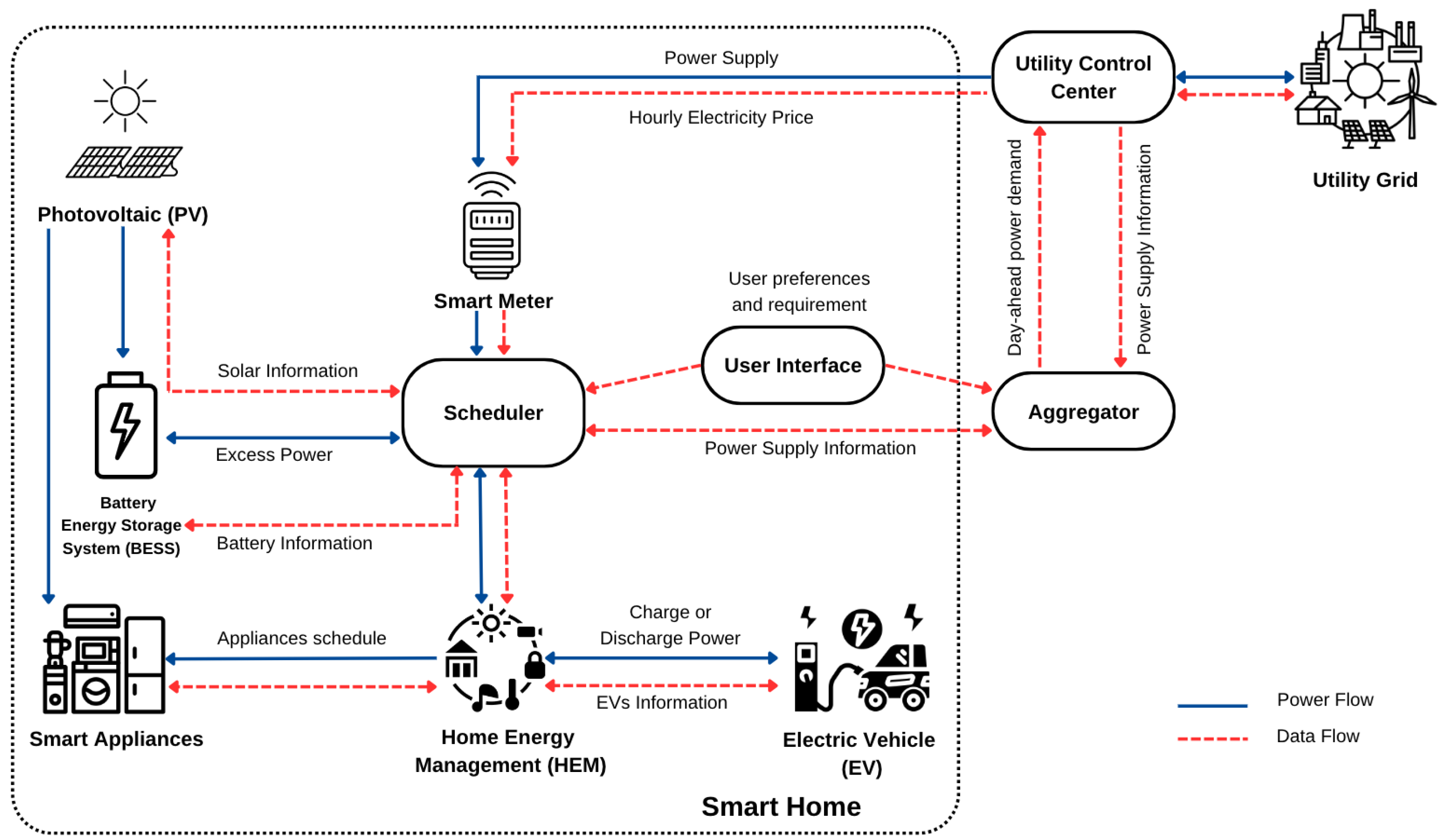
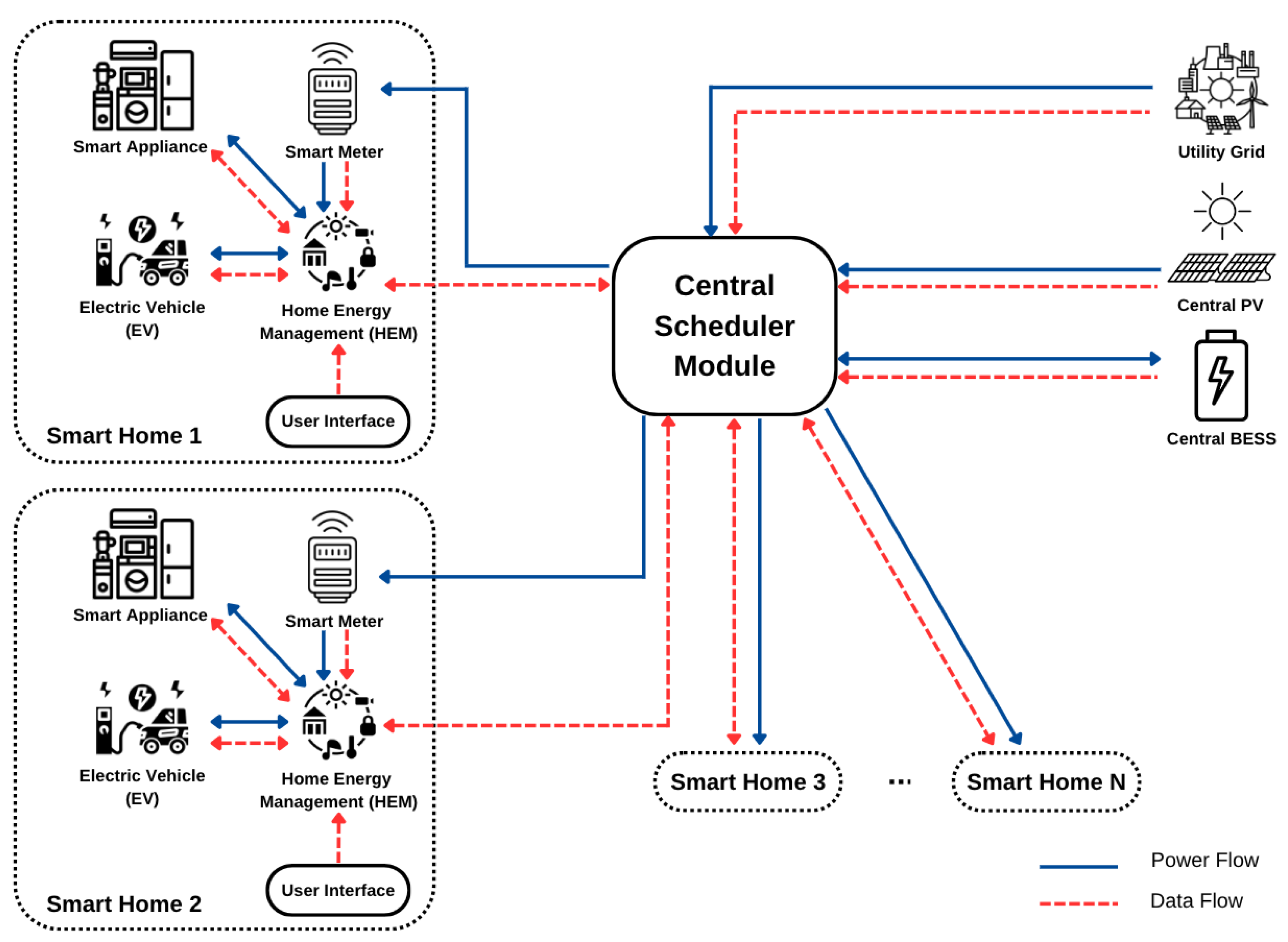
The remaining sections of this paper are organized as follows. In Section 2, we provide a brief description of our proposed system. The proposed HEM system, along with our mathematical model and objective function, is described in Section 3. We present our simulation results and discuss them in Section 4, while our conclusions are included in Section 5.

2. System Overview

The architecture of an individual SH in a distributed system is explained in Figure 1. In this system, an SH is connected to an aggregator to share its power demand information with the utility grid. This information is the expected power demand from the users for the following day. The aggregator calculates the total power demand and transmits it to the utility grid to supply power the next day. The SH system has several components installed including a smart meter, user interface, scheduler module, HEM, smart appliances, PV panels, a BESS, and EVs.

A smart meter installed at an SH is responsible for receiving the power supply from the utility grid and hourly electricity prices for the following day from the utility control center. The smart meter provides accurate and timely data to ensure efficient and effective scheduling of power usage [1]. Similarly, users provide their preferences and requirements on how they use smart appliances through a user interface. In case users do not provide information for the following day, historical data for the same day of the week will be used. This information from the smart meter and user interface works as input data to the scheduler module. To minimize the cost of electricity per day, the scheduler module optimizes the scheduling of home appliances and determines the best charge and discharge pattern of the BESS and EVs. It takes input information from a smart meter, user interface, PV, and BESS, and employs an optimization method to achieve this objective. At certain times of the day, in addition to the power supply from the grid, power may be sourced from a PV, which can directly feed smart appliances or store excess energy in a BESS for later use. Similarly, the discharge energy from EVs can be supplied to smart appliances or stored in a BESS when they are plugged in at home. Lastly, the BESS’s energy can be fed to smart appliances at any time until its SOC reaches the limit.

The HEM system manages the switching of appliances based on the schedule created by the scheduler. The appliances in the SH are connected to the HEM system using wired or communication systems, including WiFi, Bluetooth, and ZigBee. The HEM system also manages the charging and discharging of a BESS and EVs based on an optimal pattern determined by the scheduler module. There are two types of smart appliances: flexible and non-flexible. Flexible appliances can be scheduled to operate at different times throughout the day, but they must still run for the specified amount of time set by the user. Non-flexible appliances, on the other hand, cannot be scheduled and must run according to the user’s requirements without any flexibility. According to a study by Unbound Solar Home Appliances [28], we can categorize these appliances into two types and determine their average power consumption from flexible appliances (washing machines, dishwashers, clothes dryers, vacuum cleaners, and water heaters) and non-flexible appliances (air conditioners, refrigerators, electric ovens, microwaves, lights, TVs, and desktops). A rooftop PV system is the only renewable energy source in the system that generates energy that can be supplied directly to home appliances. Any excess energy produced can also be stored in a BESS. Let $E_{PV}^t$ represent the energy produced by the PV during a specific time slot t. In this work, historical data from the PV will be utilized. A BESS can be utilized to store energy generated from PV or EVs when it is not fully consumed. It can charge energy from the main grid during off-peak hours or lower electricity prices. Later, during peak hours, it can discharge the stored energy back to home appliances. It is important to note that a BESS can only discharge its stored energy to power home appliances. In this work, EVs are considered a load when they are charging and an energy storage system when they are discharging at home. V2H technology will be employed when EVs discharge energy back to a HEM. However, this is only true when the EV is at home and plugged into the HEM. During the period in which EVs are out of home, only energy discharge for traveling is considered. This means that EVs only charge their battery at home and use it for traveling and discharging back to the SH.

Power balancing is one of the major constraints for the operation of an SH. Most of the literature majorly revolves around basic equations, such as the power balancing between power generated ($P_{gen}$) and power consumed ($P_{con}$). As presented in Equation (1), $P_{gen}$ is the function of the generated power from RESs such as the photovoltage power ($P_{PV}$), the power generated from the grid ($P_{grid,sell}$), the discharging power from a BESS ($P_{BESS,dis}$), and the discharging power from an EV ($P_{EV,dis}$). In contrast, $P_{con}$ is the function of the load demand power ($P_L$), the charging power of an BESS ($P_{BESS,ch}$), the charging power of an EV ($P_{EV,ch}$), and, in some case, the power sold back to the grid ($P_{grid,buy}$). Since loads are classified into flexible loads (F) and non-flexible loads ($NF$), the load demand power ($P_L$) is defined as the summation of the flexible load power ($P_F$) and non-flexible load power ($P_{NF}$). From that, the general power balancing equation can be presented as in Equation (3) below [29]. These three equations can be written as follows:

$$P_{gen}=f(P_{PV},P_{grid,sell},P_{BESS,dis},P_{EV,dis})$$

(1)

$$\begin{array}{c}\hfill P_{con}=f(P_F,P_{NF},P_{BESS,ch},P_{EV,ch},P_{grid,buy})\end{array}$$

(2)

$$\begin{array}{c}\hfill P_{PV}+P_{grid,sell}+P_{BESS,dis}+P_{EV,dis}=P_F+P_{NF}+P_{BESS,ch}+P_{EV,ch}+P_{grid,buy}.\end{array}$$

(3)

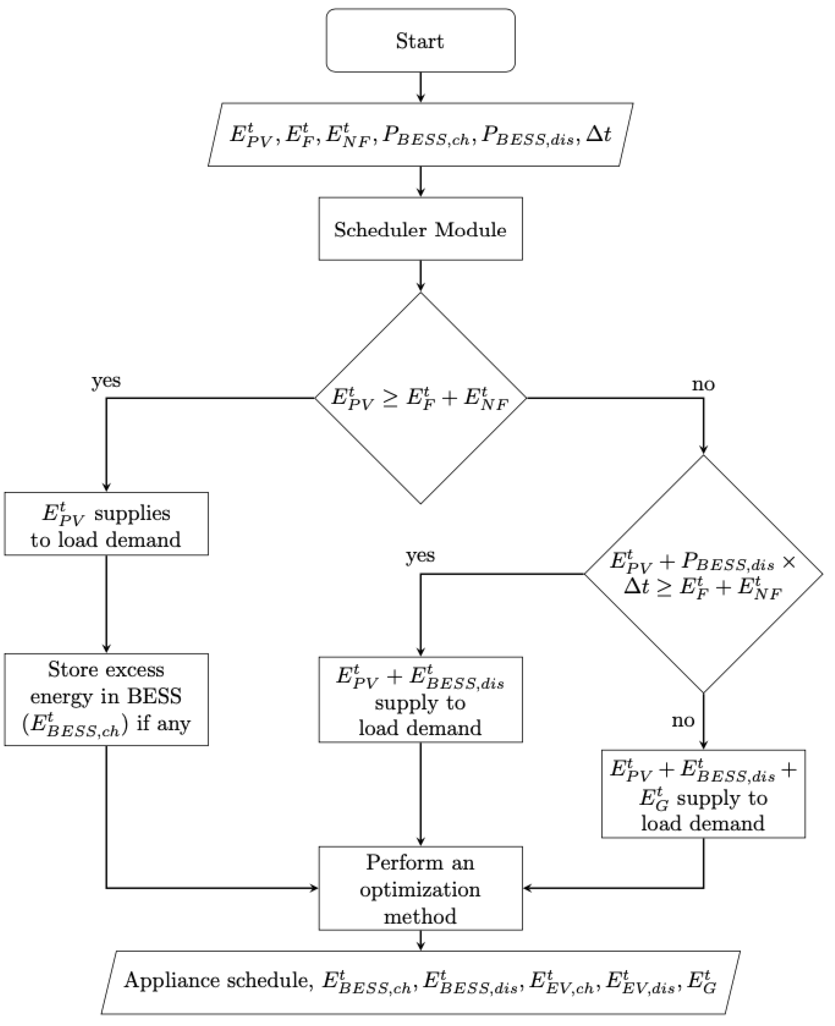
3. Proposed HEM System

In this section, a HEM system is proposed with a scheduler module that has the ability to perform an optimization method with single and multiple SHs. We define models and constraints for all elements in a SH, such as smart appliances, PVs, BESSs, and EVs. The optimization model is formulated as a MILP with all constraints being linear. Its primary objective is to minimize the total electricity cost per day for an individual SH and the accumulated total electricity cost per day for multiple SHs. The model proposes an objective function for a single SH, which is then followed by a general objective function for a centralized grid system with N number of SHs. This system includes a central PV and a central BESS that are shared among all SHs. The proposed models and constraints will ensure the efficacy and fairness in the system for all users. RTP, which is known as hourly pricing, is considered to be our electricity tariff. It is one of the most efficient tariffs compared to others in the electricity market that can inform users about the electricity price hourly or daily [30]. RTP is a pricing signal that influences users to use electricity in low-price periods. In this work, we consider the starting time of the day to be from 1 a.m. in the morning with the simulation time-step of 1 h. This means there are 24 time slots per day.

3.1. Smart Appliance

The set of flexible appliances is defined by F, and the set of non-flexible appliances is defined by $NF$. The energy consumptions in kWh of the flexible and non-flexible appliances are defined by Equations (4) and (5) below [14]:

$$E_F^t=\sum _{i\in F}[P_{i,F}\times b_{i,F}^t\times \Delta t],\forall t$$

(4)

$$E_{NF}^t=\sum _{j\in NF}[P_{j,NF}\times \Delta t],\forall t$$

(5)

where $P_{i,F}$ and $P_{j,NF}$ are the rated powers of flexible and non-flexible appliances, respectively. $\Delta t$ represents the simulation time-step (1 h), and $b_{i,F}^t$ is the binary decision variable of the flexible appliances in any time slot t. The flexible appliances are turned on when $b_{i,F}^t$ equals one and turned off otherwise.

3.2. Battery Energy Storage System

Let $E_{BESS,ch}^t$ and $E_{BESS,dis}^t$ be the energy of the BESS in the charge and discharge modes, respectively, in any time slot t. The energy flow (charge or discharge) from the BESS is denoted by $E_{BESS}^t$. It is presented in Equation (6) as the subtraction of the charge energy from the discharge energy of the BESS in any time slot t. Its value is negative when the BESS is charging and positive during discharging [26]. The limitation of the charge or discharge energy is introduced in the constraints in Equations (7) and (8), where $P_{BESS,ch}$ and $P_{BESS,dis}$ are the maximum charging and discharging powers of the BESS at any time slot t, respectively [21]. $x_{BESS,ch}^t$ and $x_{BESS,dis}^t$ are the binary decision variables that are introduced in the constraint in Equation (9) to make sure that the BESS can either charge or discharge its energy in any time slot t.

$$E_{BESS}^t=E_{BESS,dis}^t-E_{BESS,ch}^t,\forall t$$

(6)

$$0\le E_{BESS,ch}^t\le P_{BESS,ch}\times \Delta t\times x_{BESS,ch}^t,\forall t$$

(7)

$$0\le E_{BESS,dis}^t\le P_{BESS,dis}\times \Delta t\times x_{BESS,dis}^t,\forall t$$

(8)

$$x_{BESS,ch}^t+x_{BESS,dis}^t\le 1,\forall t$$

(9)

To maximize the lifespan of the BESS, the constraint in Equation (10) does not allow the SOC of the BESS to drop below 20% of its total capacity, and its maximum SOC should be at 80% of its rated capacity $C_{BESS}$. Let ${\eta }_{BESS}$ be the efficiency of the BESS in the charging and discharging modes. Then, the SOC of the BESS can be updated as in Equation (11), where $SO{C}_{BEES}^{t+1}$ and $SO{C}_{BEES}^t$ are the SOCs of the BESS in the $t+1$ and t time slots, respectively [29].

$$0.2\times C_{BESS}\le SO{C}_{BEES}^t\le 0.8\times C_{BESS},\forall t$$

(10)

$$SO{C}_{BEES}^{t+1}=SO{C}_{BESS}^t+E_{BESS,ch}^t\times {\eta }_{BESS}-E_{BESS,dis}^t/{\eta }_{BESS},\forall t$$

(11)

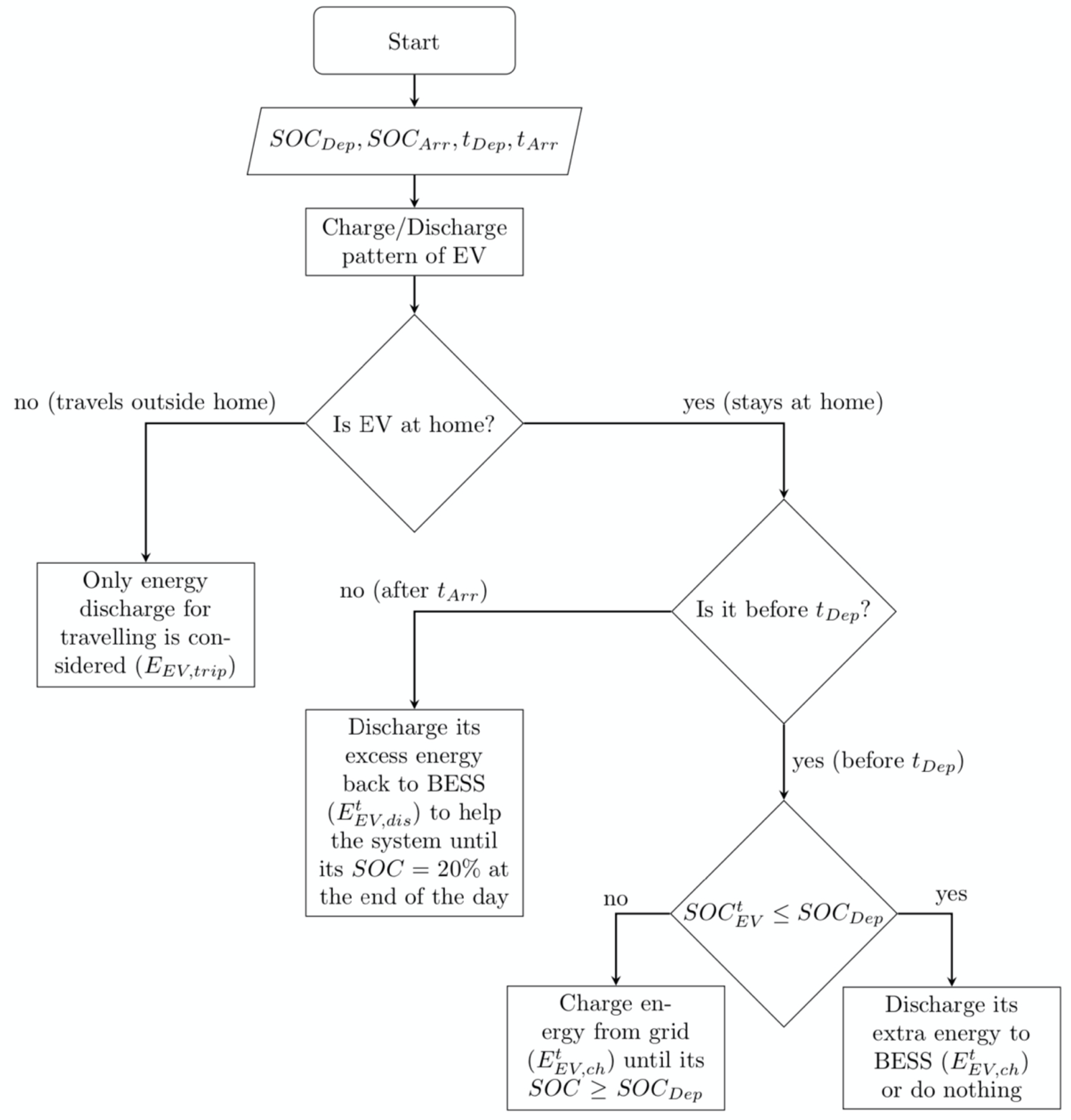
3.3. Electric Vehicle

Denote $E_{EV,ch}^t$ and $E_{EV,dis}^t$ as the charge and discharge energies of an EV, respectively, during the time that the EV is at home. Additionally, let $E_{EV}^t$ be the energy flow (charge or discharge) of the EV during the time that the EV stays at home, which is calculated using Equation (12). Its value is negative when charging and positive when discharging. To make sure that there is enough charge to cover the next trip, the SOC of the EV at the departure time ($SO{C}_{EV}^{t_{Dep}}$) has to be greater than or equal to the trip’s SOC ($SO{C}_{Dep}$), which is specified by the user [26]. This constraint is introduced in Equation (13). These two equations are specified as follows:

$$E_{EV}^t=E_{EV,dis}^t-E_{EV,ch}^t,\forall t\in [t_{Arr},t_{Dep})$$

(12)

$$SO{C}_{EV}^t\ge SO{C}_{Dep},t=t_{Dep}$$

(13)

where $t_{Dep}$ and $t_{Arr}$ represent the departure time and the arrival time of EV, respectively, and these values can be specified by the users. We assume that users plug in the EV’s charger to the HEM as soon as they arrive home at the time $t_{Arr}$.

Similar to the constraints of the BESS in Equations (7)–(9), the charge limitation constraint, discharge limitation constraint, and lifespan constraint of the EV are introduced accordingly in Equations (14)–(16) below. However, these constraints are considered when the EV is at home and the maximum charging of EVs is up to 100% of their rated battery capacity $C_{EV}$. However, the constraint in Equation (17) makes sure that EVs either charge or discharge their energy in any time slot t. These equations are shown as follows:

$$0\le E_{EV,ch}^t\le P_{EV,ch}\times \Delta t\times x_{EV,ch}^t,\forall t\in [t_{Arr},t_{Dep})$$

(14)

$$0\le E_{EV,dis}^t\le P_{EV,dis}\times \Delta t\times x_{EV,dis}^t,\forall t\in [t_{Arr},t_{Dep})$$

(15)

$$0.2\times C_{EV}\le SO{C}_{EV}^t\le C_{EV},\forall t\in [t_{Arr},t_{Dep})$$

(16)

$$x_{EV,ch}^t+x_{EV,dis}^t\le 1,\forall t\in [t_{Arr},t_{Dep})$$

(17)

where the SOC of the EV’s battery at any time slot t is represented as $SO{C}_{EV}^t$. The notations $P_{EV,ch}$ and $P_{EV,dis}$ represent the maximum charging and discharging power of the EV’s battery, respectively. Last, denote $x_{EV,ch}^t$ and $x_{EV,dis}^t$ as the binary decision variables to make sure that EVs can either charge or discharge their energy during the time slot t.

The discharging energy for the period during which EVs are out of home is denoted by $E_{EV,trip}^t$. Equations (18) and (19), below, show the limitations of discharging and constraints on the binary decision variables during the time in which EVs are on the trip, respectively.

$$0\le E_{EV,trip}\le P_{EV,dis}\times \Delta t\times x_{EV,dis}^t,\forall t\in [t_{Dep},t_{Arr})$$

(18)

$$x_{EV,dis}^t=1,\forall t\in [t_{Dep},t_{Arr})$$

(19)

Lastly, the updated SOC of the EV’s battery in any time slot t is presented in Equation (20) where ${\eta }_{EV}$ is the efficiency in the charging and discharging modes of the EVs.

$$SO{C}_{EV}^{t+1}=SO{C}_{EV}^t+E_{EV,ch}^t\times {\eta }_{EV}-E_{EV,dis}^t/{\eta }_{EV}-E_{EV,trip}^t/{\eta }_{EV},\forall t$$

(20)

The flowchart in Figure 2 represents the logic of the charge and discharge pattern of the EV used in the simulation.

The inputs for the model are $SO{C}_{Dep},SO{C}_{Arr},t_{Dep},and{t}_{Arr}$. When the EV travels out of the SH, only the energy discharge for the trip ($E_{EV,trip}$) is considered. When the EV stays at home, at the arrival time, it will discharge its excess energy from traveling back to the BESS ($E_{EV,dis}^t$) to help the system until it reaches the limit at $20\%$ of its SOC. Lastly, when the EV stays at home before the departure time, it will charge energy from the grid ($E_{EV,ch}^t$) to reach the desired SOC for traveling defined by the user ($SO{C}_{Dep}$). However, in the case that its SOC is more than the SOC for traveling, it can discharge its extra energy to the BESS or take no action depending on the system’s need.

3.4. Objective Function for a Single SH

Following the aforementioned formulas and constraints, the objective function of a single SH can be formulated as the MILP model with all constraints being linear constraints. The primary objective is to minimize the total electricity cost per day. It is defined as the sum of the total electricity consumption from the grid multiplied by the real-time electricity price for a whole day. The total electricity withdrawn from the grid per day is defined by Equation (21) where $E_G^t$ is the total energy obtained from the utility grid at any time slot t. This is also known as power balancing for the system, during which the energy sold back to the grid is not considered. Moreover, to ensure that, the constraint in (22) is formulated. Denote $p^t$ as the RTP tariff for a whole day. From the utility, the objective function of an individual SH can be written as in Equation (23).

$$E_G^t=E_F^t+E_{NF}^t-E_{BESS}^t-E_{PV}^t-E_{EV}^t,\forall t$$

(21)

$$0\le E_G^t,\forall t$$

(22)

$$min\sum _{t=1}^{24}(p^t\times E_G^t),\forall t$$

(23)

$$\mathrm{st}. \mathrm{Equations} (7)–(10),(13)–(19),(21), \mathrm{and} (22).$$

3.5. Objective Function for Multiple SHs

The multiple SHs architecture in a centralized grid system is illustrated in Figure 3 below. In this centralized system, there is a central BESS and a PV shared among all of the SHs in the community. The central scheduler module is connected to all N numbers of SHs and has the ability to perform an optimization method for those users. Each SH in this system is equipped with smart appliances, an EV charging hub, a smart meter, a user interface, and a HEM system.

The objective function of the central scheduler module is formulated as the MILP model with the primary objective of minimizing the aggregated electricity costs for all interconnected SHs by considering the RTP tariff from the utility ($p^t$). This is defined in the equation below:

$$min\sum _{i=1}^N\left(C_i\right)=min\sum _{i=1}^N\sum _{t=1}^{24}(p^t\times E_{G,i}^t),\forall t$$

(24)

where $C_i$ and $E_{G,i}$ are the total electricity price and energy withdrawal from the grid of SH $ith$, respectively, while N represents the total number of SHs in the system. The central BESS has to follow the constraints in Equations (7)–(10) and the EV in each SH has to follow the constraints in Equations (13)–(19), as in the case for the single SH in the previous section.

The energy derived from central PV sources is universally accessible to the households, with those equipped with a greater number of appliances having the capacity to harness increased energy from the PV system. In order to guarantee regulated distribution and prevent any single residence from monopolizing the energy output to the detriment of others, an additional constraint is introduced in Equation (25). This constraint mandates that each household draw energy within an equal maximum limit, thereby ensuring the impartial sharing of energy derived from the central PV system. In the case that one SH is expected not to consume energy at all, it will be excluded from the scheduling process, and the available power from the PV will be shared only among the other SHs. This means that the total number of SHs is reduced by one in the simulation. This is introduced as follows:

$$\sum _{t=1}^{24}\left(E_{PV,i}^t\right)\le (1/N)\times \sum _{t=1}^{24}\left(E_{CPV}^t\right),i=\{1,2,3,.....,N\}$$

(25)

where $E_{PV,i}^t$ is the energy withdrawn from the central PV for each home in each time slot t, and $E_{CPV}^t$ is the energy produced from the central PV in each time slot t. Additionally, it is important to note that fairness in the BESS and EV is not prioritized, as their initial and final energy levels remain the same. Essentially, these systems are designed to help manage energy use when electricity prices are high. They take advantage of lower-cost charging times to make appliances more flexible and reduce overall electricity expenses.

Figure 4 represents the flowchart of the scheduler module which is illustrated in Figure 1 and Figure 3. The scheduler module takes input parameters such as $E_{PV}^t$, $E_F^t$, $E_{NF}^t$, $P_{BESS,ch}$, $P_{BESS,dis}$, and $\Delta t$. It should be noted that an EV is considered a flexible load while charging and a BESS while discharging. The system first considers whether there is enough energy from PV generation for the load demand. If yes, ($E_{PV}^t$) will be used to supply the load demand and store excess energy in the BESS ($E_{BESS,ch}^t$). Then, the optimization will be performed. In case there is not enough PV energy for the load demand, the available power in the BESS will be considered. If the maximum discharging of the BESS and the available power from the PV are enough to supply the load demand, the power from the grid is unnecessary. Otherwise, the power from the grid ($E_G^t$) will be used to fulfill the load demand on top of that. The next step is to perform the optimization method. As the output result, the appliance schedule, $E_{BESS,ch}^t$, $E_{BESS,dis}^t$, $E_{EV,ch}^t$, $E_{EV,dis}^t$, and $E_G^t$ are obtained.

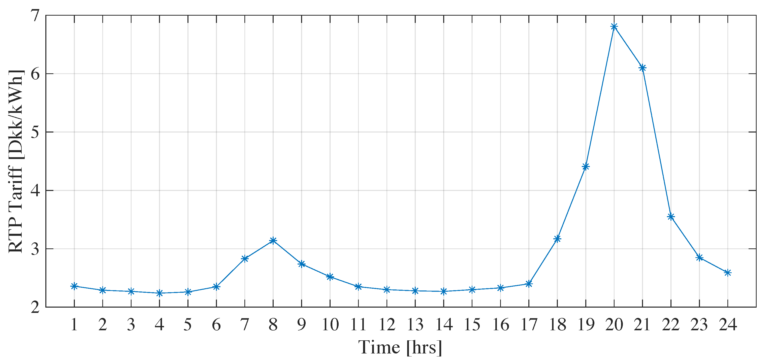
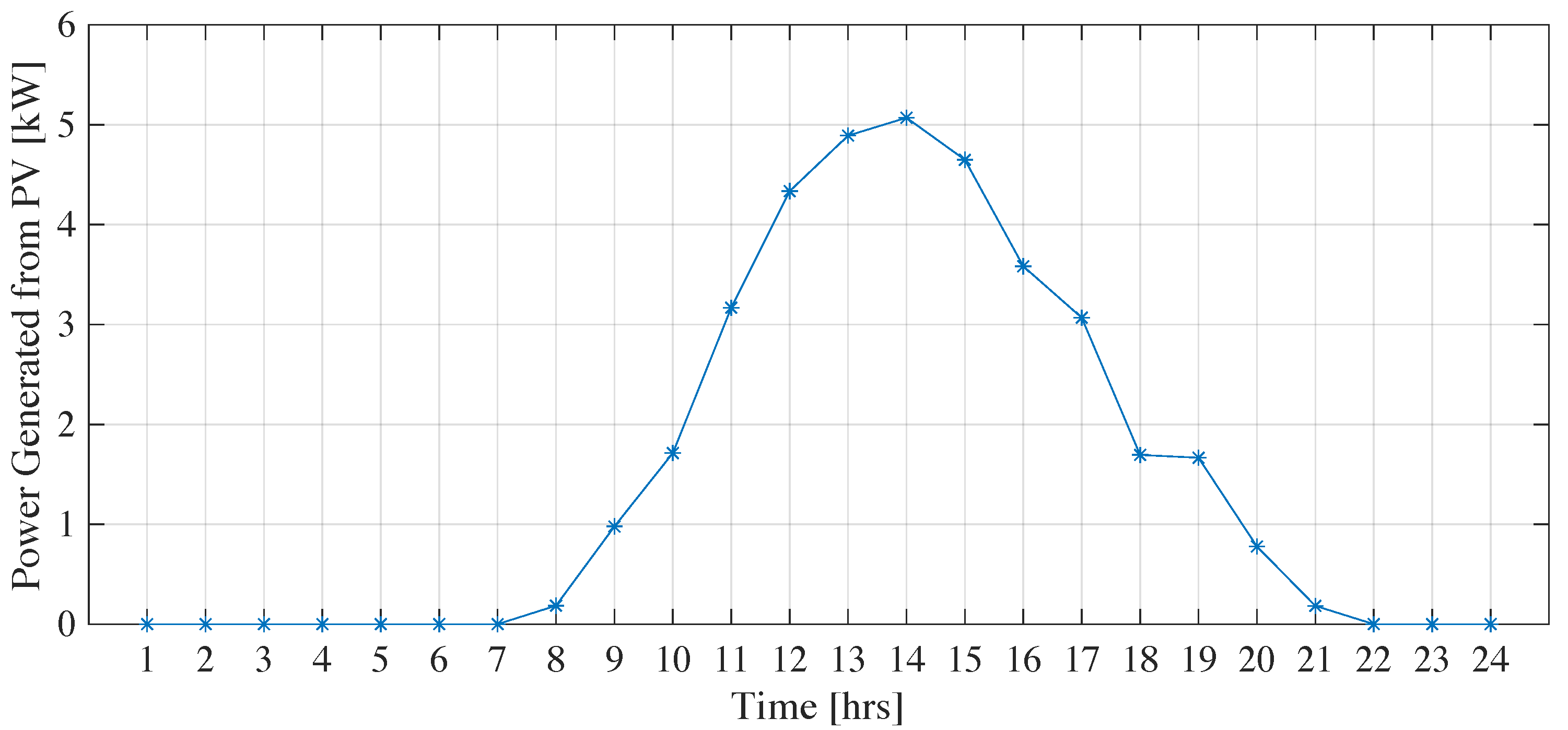
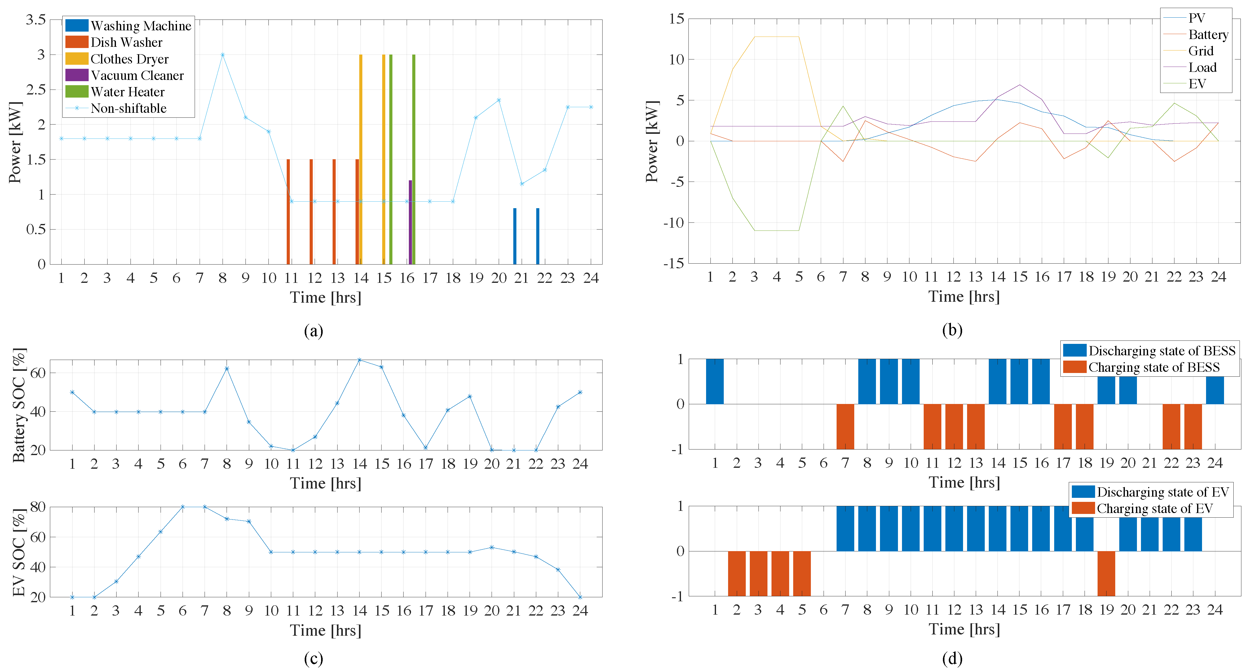
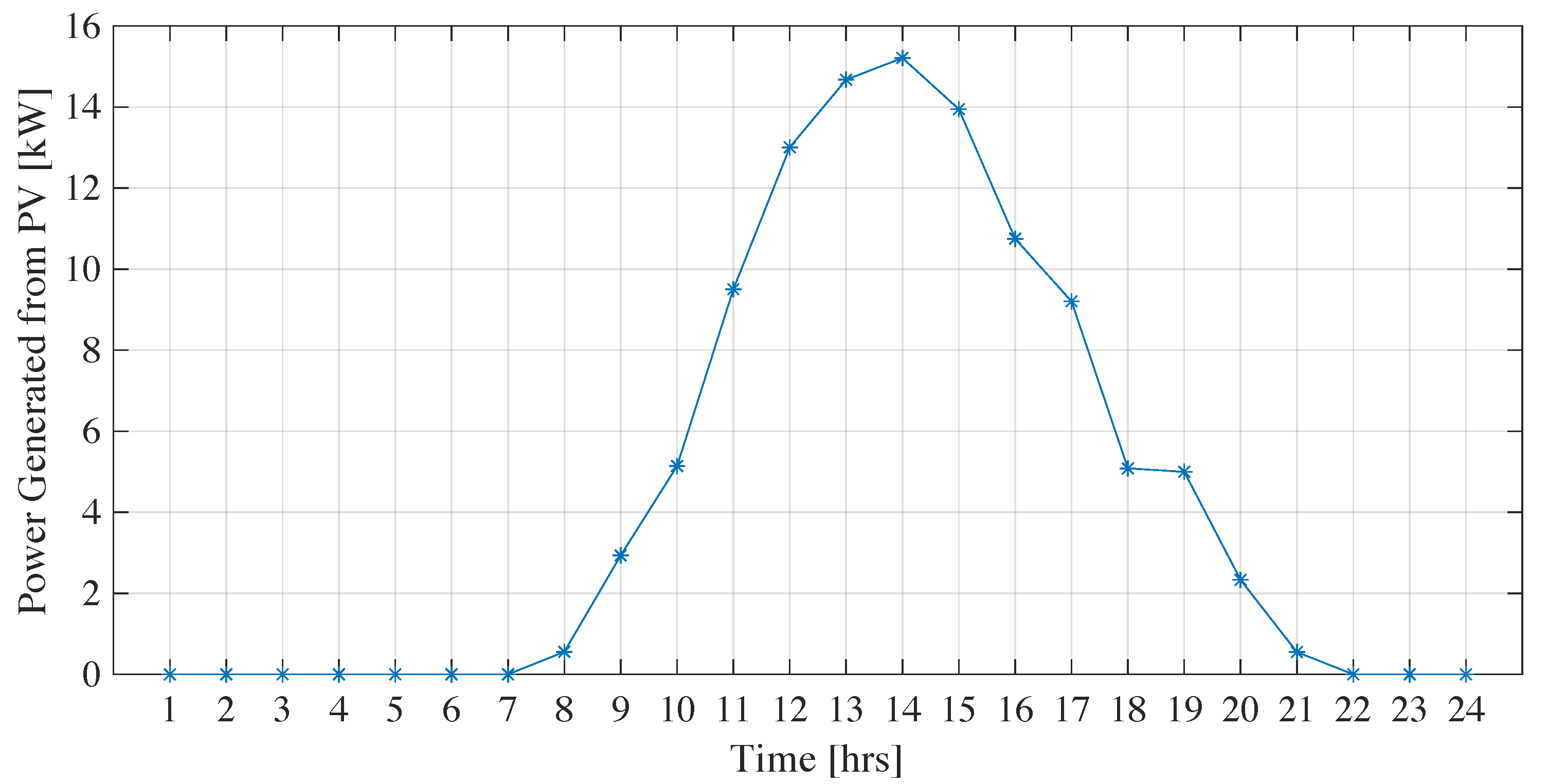
4. Results and Discussion

This section presents the data and results of our simulation that considers the energy usage of smart appliances, as well as the power flow of a PV, a BESS, and EVs. The proposed HEM system is designed in two case scenarios. The first one is the case for an individual SH, which is based on the architecture in Figure 1. A single SH has many components, such as smart appliances, a PV, a BESS, and EVs. The result will show the optimal schedule for smart appliances, along with the optimal charge and discharge pattern of the BESS and EV in that individual SH to ensure the minimum total electricity price per day. The second one is the case in which there are multiple SHs shared together with the PV and BESS in a centralized system. This simulation is based on an architecture in Figure 3. Each SH is interconnected with a central scheduler module, where there are a central PV and a BESS shared among them. The result will provide the optimal schedule for smart appliances and the optimal charge and discharge pattern of the EVs in each SH, along with its minimum total electricity cost per day. The power flow of the central PV and BESS will also be presented, along with the optimized accumulated total electricity cost of all SHs for a whole day.

The HEM system proposed in the previous section can be validated using the MILP technique for these two case scenarios. The RTP tariff is obtained from the Danish utility provided by Andel Energi [31]. The unit of electricity is $DKK$ per kWh. These data are chosen from electricity prices on 11 September 2023 and are shown in Figure 5 below.

4.1. Case Study 1: Individual SH

The focus of this study is to optimize the total electricity cost per day of a single SH. By considering an SH equipped with smart appliances, a PV, a BESS, and an EV, the data sets of these components are obtained as follows.

Table 1. Appliance preference for case study 1.

Load Type	Appliance	Power Rating [kW]	Daily Usage [hour]	Start-End Time
Flexible	Washing Machine	0.8	2	-
	Dishwasher	1.5	4	-
	Clothes Dryer	3	2	-
	Vacuum Cleaner	1.2	1	-
	Water Heater	3	2	-
Non-flexible	Air Conditioner	0.9	10	(1 a.m.–8 a.m.), (10 p.m.–12 a.m.)
	Refrigerator	0.9	24	-
	Electric Oven	1.2	4	(7 a.m.–9 a.m.), (6 p.m.–8 p.m.)
	Microwave	1	1	(9 a.m.–10 a.m.)
	Light	0.1	5	(7 p.m.–12 a.m.)
	TV	0.15	5	(7 p.m.–12 a.m.)
	Desktop	0.2	3	(9 p.m.–12 a.m.)

shows a list of smart appliances with their rated power and user preferences, such as daily usage time and the start–end time of all appliances. In the table, there are two types of smart appliances, which include five flexible appliances (washing machine, dishwasher, clothes dryer, vacuum cleaner, and water heater) and seven non-flexible appliances (air conditioner, refrigerator, electric oven, microwave, light, TV, and desktop). The historical data of the PV used in this simulation are obtained from the IEEE Open data sets [32] on the residential solar rooftop panels, which have a rated power of 10 kWh. The numerical data used for this simulation are depicted in Figure 6.

The specifications of the BESS and EV are obtained from the IEEE Open data sets [32], which can be described as follows. The capacity of the BESS is 10 kWh with a maximum charging and discharging rate of 2.5 kW, and the efficiency in charging and discharging is 90%. We assume that the SOC of the BESS at the start and the end of the day (i.e., midnight) is equal to 50% of its total capacity, which is 5 kWh. The model of the EV used in this case study is a Tesla Model S, which has a battery capacity of 60 kWh with a maximum charge and discharge power of 11 kW, and the efficiency of the EV’s battery in charging and discharging is 90%. We assume that the initial and final SOC of the EV at the start and end of the day (i.e., midnight) is equal to 20% of its battery’s capacity. The driving activities of the EV’s user on a working day were chosen from an EV user in the IEEE Open data sest [32] and can be described as follows. The driver leaves home at 8 a.m. in the morning with at least 80% of the EV’s SOC and arrives home from work at 7 p.m. in the evening with a percentage of the EV’s SOC of 50%.

The simulation result is shown in Figure 7 with four sub-figures depicted. The optimal schedule for the smart appliances is illustrated in Figure 7a. Since non-flexible appliances cannot be scheduled and have to follow exactly the user preference, the total consumption of all seven non-flexible appliances is shown in one curve. The bar graphs in the same figure represent the minimum schedule for the flexible appliances. It can be noticed that most flexible appliances were scheduled in the afternoon time, from 11 a.m. to 5 p.m., which is due to the lower electricity price and the higher generated power from the PV during that time. However, the washing machine, on the other hand, was scheduled to operate at 9 p.m. and 10 p.m., which is the peak time of the electricity price. This is because, during that period of time, the total consumption of the non-flexible appliances is low, and the EV is plugged-in at home to discharge its excess power from traveling back to the system.

Figure 7b presents the power flow in the system among the load, grid, PV, BESS, and EV. Load demand from smart appliances is mostly sourced from the PV around daytime when there is high irradiation. The rest of the time, it relies on the power supply from the utility grid and the BESS. This is the same for our system; at the start of the day, between 1 a.m. and 7 p.m., power from the utility grid was fed for load demand, and, during mid-day, power was sourced from the PV instead. It can be noticed that the grid power was charged into the EV’s battery mostly at the start of the day since the EV needed enough energy for traveling before its departure time at 8 a.m., and electricity prices at that time were low. The EV mainly helped the system after it arrived home at 7 p.m. during the peak hour of electricity prices. The excess energy in the EV’s battery after traveling was discharged to the BESS to help feed to load demand and avoid using power from the main grid. Finally, the BESS was responsible for storing the energy from the grid during the off-peak time and discharging it back to the load demand during the on-peak time. The excess power from the PV was also charged to the BESS, such as between 10 a.m. and 1 p.m., and the BESS’s power was supplied back to the load appliance when there was not enough generated power from the PV, such as from 2 p.m. to 4 p.m.

The SOC and the charging or discharging status of the BESS and EV are depicted in Figure 7c and Figure 7d, accordingly. We can see that the SOC of the EV was increasing rapidly during the start of the day, which went from 20% initially up to 80% at 6 p.m. before its departure time at 8 a.m. Then, it decreased while the EV was traveling to 50% when it arrived home at 7 p.m. After the EV arrived home, its SOC dropped until the end of the day with 20% of its battery capacity. Unlike the EV, the BESS has been physically equipped at home and is able to help the system for the whole day. The energy in the BESS was initially at 50% SOC, and then it increased or decreased depending on the system. Later, the BESS’s SOC was back to 50% at the end of the day, and this amount of energy was kept as the initial SOC for the next day. The charging or discharging status of the BESS and EV are presented as a bar graph in which a positive value means the BESS or EV discharged at a specific time, and the negative value means otherwise. The meanings of the positive values and negative values were used to follow the value of the energy flow of the BESS ($E_{BESS}^t$) and the energy flow of the EV ($E_{EV}^t$), as presented previously in Section 3. At one specific time, the BESS and EV were considered to charge (negative value), discharge (positive value), or take no action (zero value). For simplicity in the simulation, the EV was considered discharged only during the period that it was traveling.

The result of the optimization model on an individual SH showed a significant reduction in the total electricity cost compared to the case of a traditional SH. The term traditional SH refers to a home that incorporates smart or automated technologies to enhance various aspects of daily living. A traditional SH is usually equipped with a HEM system, which is able to schedule smart devices only. The integration of a PV, BESS, and EV is not included in that system due to the complexity in scheduling. The proposed HEM system in this work with a MILP technique provided a minimum schedule for smart appliances along with the optimal charging and discharging patterns of the BESS and EV. This was presented with the objective value for the total electricity cost per day, which is equal to $114.11DKK$. As presented in

Table 2. Comparison result for individual SH case study.

Total Cost of Traditional SH	Total Cost of Proposed HEM	Reduction
$164.03DKK/$day	$114.11DKK/$day	30.43%

, this amount shows a reduction of 30.43% compared to the case of the traditional SH with $164.03DKK$ per day.

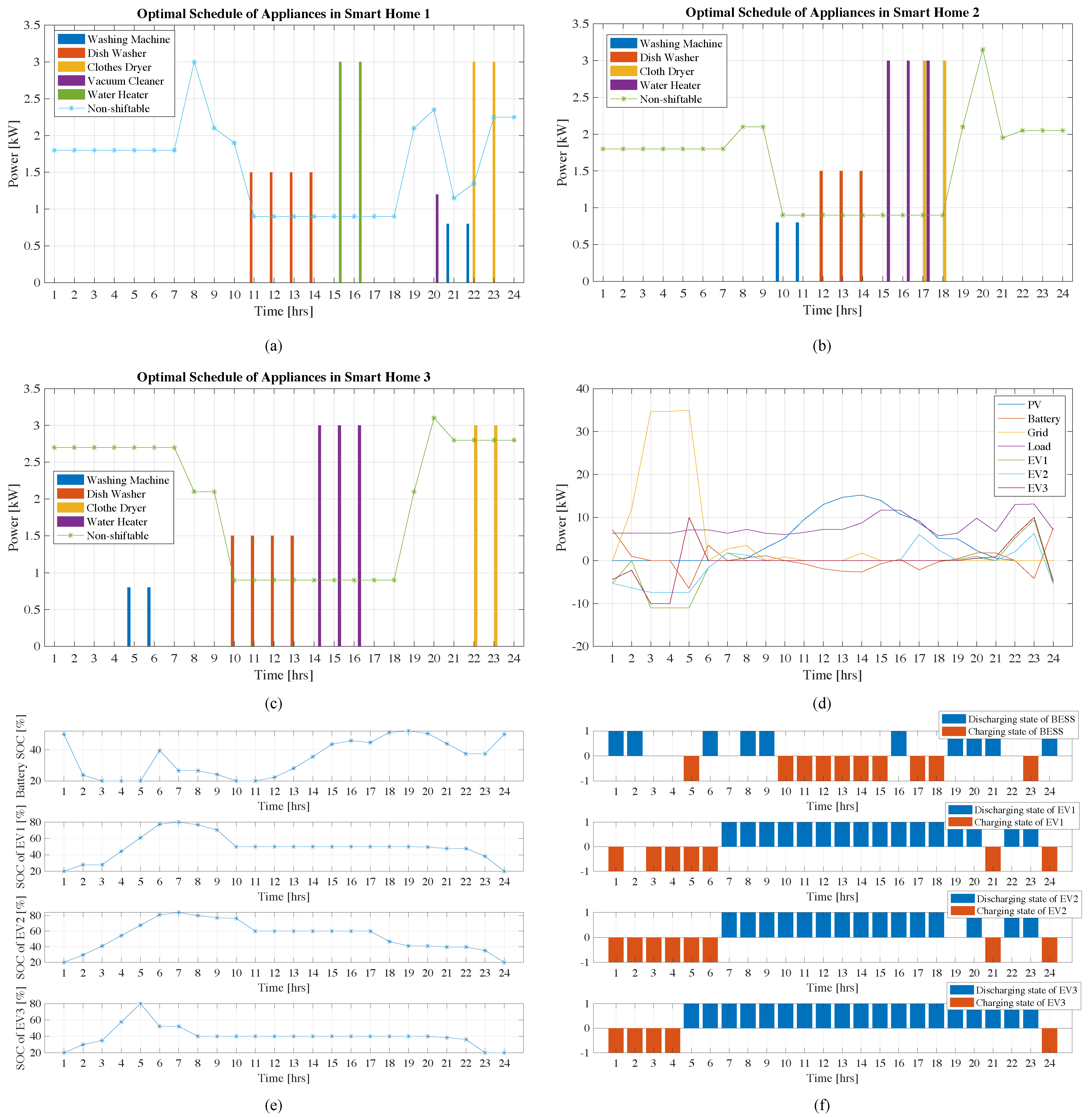
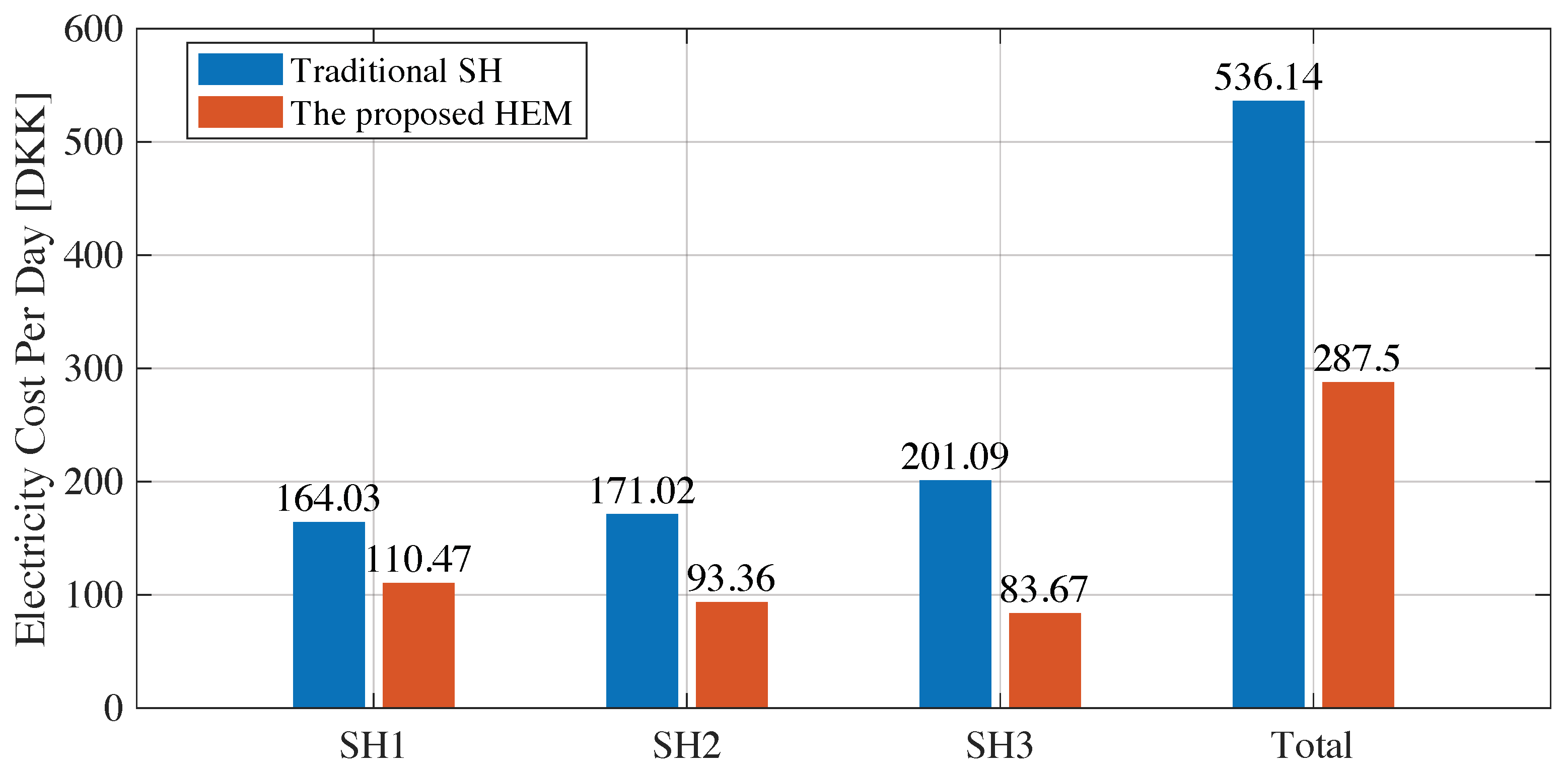
4.2. Case Study 2: Multiple SHs

For this case study, we consider a case of an apartment building that consists of three SHs. Each SH is connected to a central scheduler module of the apartment and shares the usage of the PV and BESS. The components included in each SH are a smart meter, smart appliances, a user interface, an EV, and a HEM. We considered that each user owns an EV in their SH with different specifications and models.

The data sets of the central PV and BESS were obtained from the IEEE Open data sets [32], which can be described as follows. The rated power of the PV is 30 kWh and its generated power is depicted in Figure 8 below. The central BESS has a rated power of 30 kWh with maximum charging and discharging of $7.5$ kW, and the efficiency in charging and discharging is 90%. Similar to the case of the individual SH, the initial and final SOC of the BESS was considered 50% of its capacity.

The appliance preferences of SH1 were kept the same as in the previous case study, which is presented in Table 1, while the appliance preferences of SH2 and SH3 are presented in

Table 3. Appliance preference in SH 2.

Load Type	Appliance	Power Rating [kW]	Daily Usage [hour]	Start-End Time
Flexible	Washing Machine	0.8	3	-
	Dishwasher	1.5	3	-
	Clothes Dryer	3	2	-
	Water Heater	3	3	-
Non-flexible	Air Conditioner	0.9	12	(1 a.m.-8 a.m.), (7 p.m.–12 a.m.)
	Refrigerator	0.9	24	-
	Electric Oven	1.2	4	(7 a.m.-9 a.m.), (6 p.m.–8 p.m.)
	Light	0.1	3	(9 p.m.–12 a.m.)
	TV	0.15	5	(7 p.m.–12 a.m.)

and

Table 4. Appliance preference in SH 3.

Load Type	Appliance	Power Rating [kW]	Daily Usage [hour]	Start-End Time
Flexible	Washing Machine	0.8	2	-
	Dishwasher	1.5	4	-
	Clothes Dryer	3	2	-
	Water Heater	3	3	-
Non-flexible	Air Conditioner 1	0.9	10	(1 a.m.–8 a.m.), (10 p.m.–12 a.m.)
	Air Conditioner 2	0.9	12	(1 a.m.–8 a.m.), (7 p.m.–12 a.m.)
	Refrigerator	0.9	24	-
	Electric Oven	1.2	4	(7 a.m.–9 a.m.), (6 p.m.–8 p.m.)
	Light	0.1	5	(7 p.m.–12 a.m.)

, respectively. Similarly, the specification and driving activities for the EV used in SH1 were maintained as in the previous case and are now presented alongside the specifications for the EVs used in SH2 and SH3. All of the specifications and driving activities for the EVs in these three SHs were obtained from the IEEE Open data sets [32] and are listed in

Table 5. Specification and driving activity of EV.

Type	Parameter	SH 1	SH 2	SH 3
Specification	Model of EV	Tesla Model S	Peugeot	Toyota Rev4 EV
	$C_{EV}$	60 kWh	50 kWh	40 kWh
	Initial and Final $SO{C}_{EV}$	$20\%$	$20\%$	$20\%$
	$P_{EV,ch}/P_{EV,dis}$	11 kW	$7.4$ kW	10 kW
	${\eta }_{EV}$	$90\%$	$90\%$	$90\%$
Driving Activity	$t_{Dep}$	8 a.m.	9 a.m.	6 a.m.
	$SO{C}_{Dep}$	$80\%$	$80\%$	$80\%$
	$t_{Arr}$	7 p.m.	5 p.m.	8 p.m.
	$SO{C}_{Arr}$	$50\%$	$60\%$	$40\%$

.

The simulation result of case study 2 is shown in Figure 9. The optimal schedules of smart appliances in each SH are depicted in Figure 9a, Figure 9b, and Figure 9c for SH numbers 1, 2, and 3, respectively.

The non-flexible appliances were shown together as a total consumption in one line, and the flexible appliances were depicted separately as a bar graph. It can be noticed that most of the flexible appliances in those three SHs were scheduled at mid-day. This is due to the high power generated from the central PV and the low electricity prices for that period. However, as depicted in Figure 9a, some flexible appliances in SH1, such as the vacuum cleaner, washing machine, and clothes dryer, were shifted to use at night between 8 p.m. to 11 p.m. Similarly, as shown in Figure 9c, some flexible appliances, such as washing machines and clothes dryers, were scheduled to be used in the morning and at night, respectively. The reason that these appliances were scheduled outside the mid-day time, when there is available power from PV, is that, in the morning, the EV was at home, and, also, the electricity price is low. Similarly, at night, the EVs were all at home to help the system along with the BESS. The power flow in the system is illustrated in Figure 9d, which presents the total power generated from the central PV; the power flow of the central BESS; and the power withdrawal from the grid, load demand, and power flow of each EV. The central PV generated more power than load consumption from 10 a.m. to 4 p.m., which provides excess power to store in the BESS. At the start of the day, when the electricity price was low, most of the load demand was fed by the grid power. In contrast, from 3 p.m. to 12 p.m., there was no use of the grid power since there was a high generation from the PV, and the EVs were available at home. The help from the EVs around that time can help avoid using power from the grid and reduce total electricity costs since it is at the on-peak time with high electricity prices. The same as in the individual SH case study, the EVs were charged at the start of the day until their SOC reached the desired percentage before their departing time. Then, when they arrived home, the EVs were considered as a BESS with their excess power in the batteries until the end of the day. The SOCs of the central BESS and the EVs in all three SHs are shown in Figure 9e. The BESS’s SOC started at 50% at the beginning of the day, and, after the BESS was charged or discharged to help the system throughout the day, its SOC came back at 50% at the end of the day. Similarly, each EV was charged at the beginning of the day until it had enough power to travel, which was at least 80% before departure. Then, their SOC returned to $20\%$ at the end of the day after their excess energy was discharged to help the grid system. Lastly, the charging and discharging status of the BESS and EVs are depicted in Figure 9f.

The result of an optimization model on the multiple SHs case study has shown a significant reduction in the total electricity cost per day of an individual SH and three SHs altogether. Figure 10 provides a bar chart comparing the total costs for the traditional SH case with the proposed HEM system. There are reductions in the total electricity cost per day in the amounts of 32.65%, 45.41%, 58.39%, and 46.38% in the case of SH1, SH2, SH3, and altogether, respectively. These amounts of reduction show that the proposed HEM system can outperform the traditional SH by achieving the flexibility assessment of the PV and the optimal planning of the BESS and EV. Further, the result shows that each SH has withdrawn the same amount of power from the central PV per day, which is equal to $35.247$ kW. This shows the significant output to ensure fairness for all users in the system as proposed.

5. Conclusions

By automatic optimization of the electricity loads in SHs, both end users and utilities will benefit from electricity cost reduction and grid services. In this paper, multiple SHs equipped with a BESS, a PV, an EV, and appliances are considered for the application of a MILP approach to minimize electricity costs. The optimization model factors in RTP tariffs and delivers efficient scheduling of appliances, as well as the optimal BESS and EV charging and discharging patterns. The simulation encompasses various scenarios accounting for diverse user preferences and consumption patterns. Furthermore, it extends to multiple SHs sharing the same system, BESS, and PV, promoting economic equity and fairness across these residences. Both individual and multiple SH case studies experience significant reductions in electricity costs. The corresponding simulation results show that the use of the proposed HEM strategy in multiple SHs could reduce the electricity cost by 46.38%. Finally, it can be concluded that the proposed method for the SHs with an EV and PV provides better results than the SHs without a PV and EV in terms of electricity cost reduction.

References

1. Panda, S.; Mohanty, S.; Rout, K.; Sahu, B.K.; Bajaj, M.; Zawbaa, H.M.; Kamel, S. Residential Demand Side Management model, optimization and future perspective: A review. Energy Rep. 2022, 8, 3727–3766. [Google Scholar] [CrossRef]
2. Hussain, H.M.; Narayanan, A.; Sahoo, S.; Yang, Y.; Nardelli, P.H.; Blaabjerg, F. Home Energy Management Systems: Operation and Resilience of Heuristics Against Cyberattacks. IEEE Syst. Man Cybern. Mag. 2022, 8, 21–30. [Google Scholar] [CrossRef]
3. Judge, M.A.; Khan, A.; Manzoor, A.; Khattak, H.A. Overview of smart grid implementation: Frameworks, impact, performance and challenges. J. Energy Storage 2022, 49, 104056. [Google Scholar] [CrossRef]
4. International Energy Agency—iea.org. Available online: https://www.iea.org/ (accessed on 3 November 2023).
5. Al-Sorour, A.; Fazeli, M.; Monfared, M.; Fahmy, A.A. Investigation of Electric Vehicles Contributions in an Optimized Peer-to-Peer Energy Trading System. IEEE Access 2023, 11, 12489–12503. [Google Scholar] [CrossRef]
6. Siano, P. Demand response and smart grids—A survey. Renew. Sustain. Energy Rev. 2014, 30, 461–478. [Google Scholar] [CrossRef]
7. Yong, J.Y.; Ramachandaramurthy, V.K.; Tan, K.M.; Mithulananthan, N. A review on the state-of-the-art technologies of electric vehicle, its impacts and prospects. Renew. Sustain. Energy Rev. 2015, 49, 365–385. [Google Scholar] [CrossRef]
8. Hamed, S.G.; Kazemi, A. Multi-objective cost-load optimization for demand side management of a residential area in smart grids. Sustain. Cities Soc. 2017, 32, 171–180. [Google Scholar] [CrossRef]
9. Eltamaly, A.M.; Alotaibi, M.A.; Elsheikh, W.A.; Alolah, A.I.; Ahmed, M.A. Novel Demand Side-Management Strategy for Smart Grid Concepts Applications in Hybrid Renewable Energy Systems. In Proceedings of the 2022 4th International Youth Conference on Radio Electronics, Electrical and Power Engineering (REEPE), Moscow, Russia, 17–19 March 2022. [Google Scholar] [CrossRef]
10. Ali, S.; Ullah, K.; Hafeez, G.; Khan, I.; Albogamy, F.R.; Haider, S.I. Solving day-ahead scheduling problem with multi-objective energy optimization for demand side management in smart grid. Eng. Sci. Technol. Int. J. 2022, 36, 101135. [Google Scholar] [CrossRef]
11. Jindal, A.; Bhambhu, B.S.; Singh, M.; Kumar, N.; Naik, K. A Heuristic-Based Appliance Scheduling Scheme for Smart Homes. IEEE Trans. Ind. Inform. 2020, 16, 3242–3255. [Google Scholar] [CrossRef]
12. Mota, B.; Faria, P.; Vale, Z. Residential load shifting in demand response events for bill reduction using a genetic algorithm. Energy 2022, 260, 124978. [Google Scholar] [CrossRef]
13. Ahmad, A.; Khan, A.; Javaid, N.; Hussain, H.M.; Abdul, W.; Almogren, A.; Alamri, A.; Niaz, I.A. An optimized home energy management system with integrated renewable energy and storage resources. Energies 2017, 10, 549. [Google Scholar] [CrossRef]
14. Dinh, H.T.; Yun, J.; Kim, D.M.; Lee, K.H.; Kim, D. A Home Energy Management System with Renewable Energy and Energy Storage Utilizing Main Grid and Electricity Selling. IEEE Access 2020, 8, 49436–49450. [Google Scholar] [CrossRef]
15. Albogamy, F.R. Optimal Energy Consumption Scheduler Considering Real-Time Pricing Scheme for Energy Optimization in Smart Microgrid. Energies 2022, 15, 8015. [Google Scholar] [CrossRef]
16. Bouakkaz, A.; Mena, A.J.; Haddad, S.; Ferrari, M.L. Efficient energy scheduling considering cost reduction and energy saving in hybrid energy system with energy storage. J. Energy Storage 2021, 33, 101887. [Google Scholar] [CrossRef]
17. Javaid, N.; Ullah, I.; Akbar, M.; Iqbal, Z.; Khan, F.A.; Alrajeh, N.; Alabed, M.S. An Intelligent Load Management System with Renewable Energy Integration for Smart Homes. IEEE Access 2017, 5, 13587–13600. [Google Scholar] [CrossRef]
18. Abdelaal, G.; Gilany, M.I.; Elshahed, M.; Sharaf, H.M.; El’Gharably, A. Integration of Electric Vehicles in Home Energy Management Considering Urgent Charging and Battery Degradation. IEEE Access 2021, 9, 47713–47730. [Google Scholar] [CrossRef]
19. Eltamaly, A.M.; Rabie, A.H. A Novel Musical Chairs Optimization Algorithm. Arab. J. Sci. Eng. 2023, 48, 10371–10403. [Google Scholar] [CrossRef]
20. Khan, M.A.; Haque, A.; Kurukuru, V.S.B. Power Flow Management With Q-Learning for a Grid Integrated Photovoltaic and Energy Storage System. IEEE J. Emerg. Sel. Top. Power Electron. 2022, 10, 5762–5772. [Google Scholar] [CrossRef]
21. Erdinc, O.; Paterakis, N.G.; Mendes, T.D.; Bakirtzis, A.G.; Catalão, J.P. Smart Household Operation Considering Bi-Directional EV and ESS Utilization by Real-Time Pricing-Based DR. IEEE Trans. Smart Grid 2015, 6, 1281–1291. [Google Scholar] [CrossRef]
22. Hou, X.; Wang, J.; Huang, T.; Wang, T.; Wang, P. Smart Home Energy Management Optimization Method Considering Energy Storage and Electric Vehicle. IEEE Access 2019, 7, 144010–144020. [Google Scholar] [CrossRef]
23. Imran, A.; Hafeez, G.; Khan, I.; Usman, M.; Shafiq, Z.; Qazi, A.B.; Khalid, A.; Thoben, K.D. Heuristic-Based Programable Controller for Efficient Energy Management under Renewable Energy Sources and Energy Storage System in Smart Grid. IEEE Access 2020, 8, 139587–139608. [Google Scholar] [CrossRef]
24. Alfaverh, K.; Alfaverh, F.; Szamel, L. Plugged-in electric vehicle-assisted demand response strategy for residential energy management. Energy Inform. 2023, 6, 6. [Google Scholar] [CrossRef]
25. Golshannavaz, S. Cooperation of electric vehicle and energy storage in reactive power compensation: An optimal home energy management system considering PV presence. Sustain. Cities Soc. 2018, 39, 317–325. [Google Scholar] [CrossRef]
26. Chreim, B.; Esseghir, M.; Merghem-Boulahia, L. LOSISH—LOad Scheduling In Smart Homes based on demand response: Application to smart grids. Appl. Energy 2022, 323, 119606. [Google Scholar] [CrossRef]
27. Gomes, I.; Ruano, M.; Ruano, A. MILP-based model predictive control for home energy management systems: A real case study in Algarve, Portugal. Energy Build. 2023, 281, 112774. [Google Scholar] [CrossRef]
28. Home Appliances Power Consumption Table—unboundsolar.com. Available online: https://unboundsolar.com/solar-information/power-table#tablePower (accessed on 7 November 2023).
29. Khan, M.A.; Bayati, N.; Ebel, T. Techno-economic analysis and predictive operation of a power-to-hydrogen for renewable microgrids. Energy Convers. Manag. 2023, 298, 117762. [Google Scholar] [CrossRef]
30. Honarmand, M.E.; Hosseinnezhad, V.; Hayes, B.; Shafie-Khah, M.; Siano, P. An Overview of Demand Response: From its Origins to the Smart Energy Community. IEEE Access 2021, 9, 96851–96876. [Google Scholar] [CrossRef]
31. andelenergiTimeenergiPris. Timeenergi din Pris Følger Markedet Time for Time—andelenergi.dk. Available online: https://andelenergi.dk/sel/timeenergi/ (accessed on 13 September 2023).
32. PES. IEEE Open Data Sets. 2022. Available online: https://site.ieee.org/pes-iss/data-sets/#cons (accessed on 12 October 2023).
Figure 1. SH architecture.
Energies 17 00254 g001
Figure 2. The flowchart of EV model.
Energies 17 00254 g002
Figure 3. Multiple SHs architecture.
Energies 17 00254 g003
Figure 4. The flowchart of scheduler module.
Energies 17 00254 g004
Figure 5. RTP tariff.
Energies 17 00254 g005
Figure 6. Power generated from PV.
Energies 17 00254 g006
Figure 7. Simulation result of case study 1: (a) optimal schedule for smart appliances; (b) power flow in the system; (c) the SOC of BESS and EV; and (d) charging and discharging status of BESS and EV.
Energies 17 00254 g007
Figure 8. Power generated from the central PV.
Energies 17 00254 g008
Figure 9. Simulation result of case study 2: (a) optimal schedule for smart appliances in SH1; (b) optimal schedule for smart appliances in SH2; (c) optimal schedule for smart appliances in SH3; (d) power flow in the system; (e) the SOC of BESS and EVs; and (f) charging and discharging status of BESS and EVs.
Energies 17 00254 g009
Figure 10. Comparison result for multiple SHs case study.
Energies 17 00254 g010