Abstract
Electricity prices are a central element of the electricity market, and accurate electricity price forecasting is critical for market participants. However, in the context of increasingly integrated economic markets, the complexity of the electricity system has increased. As a result, the number of factors required to consider in electricity price forecasting is growing. In addition, the high percentage of renewable energy penetration has increased the volatility of electricity generation, making it more challenging to predict prices accurately. In this paper, we propose a probabilistic forecasting method based on SHAP (SHapley Additive exPlanation) feature selection and LSTNet (long- and short-term time-series network) quantile regression. First, to reduce feature redundancy and overfitting, we use the SHAP method to perform feature selection in a high-dimensional input feature set, and specifically analyze the magnitude and manner in which features affect electricity prices. Second, we apply the LSTNet quantile regression model to predict the electricity value under different quantiles. Finally, the probability density function and the prediction interval of the predicted electricity prices are obtained by kernel density estimation. The case of the Danish electricity market validates the effectiveness and accuracy of our proposed method. The accuracy of the proposed method is better than that of other methods, and we assess the importance and direction of the impact of features on electricity prices.
1. Introduction
Electricity prices are the core of the electricity market and have strong economic leverage. The fluctuations in electricity prices affect the flow and allocation of various resources in the electricity market. In the electricity market environment, accurate electricity price forecasting is of great importance to all participants in the market [1,2,3]. The increasing penetration of renewable energy in the power system has made power generation more volatile and the resulting electricity prices more unpredictable than ever before.
Existing studies on electricity price forecasting can be classified into deterministic and probabilistic forecasts based on the form of the results. Deterministic forecasts usually have a single point forecast value as output, while probabilistic forecasts can have quantile estimates, forecast interval estimates, and probability density estimates as output.
Deterministic forecasting methods include mainly statistical and artificial intelligence methods. Statistical models rely on linear regressions and represent forecasts through linear combinations of explanatory variables. They are effective when dealing with linear data but perform poorly when dealing with non-stationary and non-linear data. ARIMA (autoregressive integrated moving average model) [4,5] and GARCH (generalized autoregressive conditional heteroskedasticity) [6] are commonly used statistical models. Artificial intelligence models are better at handling non-smooth and non-linear data than statistical models, especially deep neural networks. The Recurrent Neural Network (RNN) is a powerful model for processing time series data, which achieves impressive results by constructing additional maps to preserve the information from past inputs. As important variants of RNN, LSTM (long short-term memory) and GRU (gated recurrent unit) are used to solve the gradient vanishing problem of RNN [7,8]. Reference [9] decomposed a nonlinear series of electricity prices using wavelet variations and then captured the appropriate behavior of electricity prices using an Adam-optimized LSTM model. The validity of the hybrid model was verified with Australian and French datasets. Reference [10] divided the electricity price prediction into two parts: ARIMA predicted the linear part of the electricity price series and Bi_LSTM (bidirectional long and short-term memory) predicted the nonlinear part of the electricity price series. The results of the electricity price prediction were obtained by combining the linear and nonlinear parts. Reference [11] used a new evolutionary algorithm differential evolution DE to identify suitable hyperparameters for LSTM to efficiently obtain optimal solutions for hyperparameters. Convolutional neural networks (CNNs) excel in image-related tasks, and many electricity price prediction studies use CNNs to extract time-series features [12]. Reference [13] used feature selection and feature extraction techniques to reduce the dimensionality of the input data to eliminate the redundancy of the data. Moreover, reference [13] used an enhanced convolutional neural network ECNN and enhanced support vector regression ESVR as prediction models to reduce the overfitting problem. The arithmetic examples of electricity load forecasting and tariff forecasting verify the accuracy and stability of the model. Reference [14] proposed a LSTNet model that can extract both long-term and short-term dependent patterns of electricity price sequences, where a CNN is set to extract short-term dependent patterns, and a RNN and RNN skip are set to extract long-term dependent patterns with a GRU RNN component. When compared to several state-of-the-art base-line methods, LSTNet significantly outperformed them in studies on real-world data with complicated mixtures of repetitive patterns.
Traditional research on power system forecasting is dominated by deterministic forecasting, and it is difficult to avoid forecast errors. Deterministic forecasting is difficult to apply in new energy power systems, because it is difficult to achieve quantitative analysis and estimation of the fluctuation range of forecast errors. Probabilistic forecasting, as a theory and method to quantify prediction uncertainty, can obtain the probability distribution of the predicted object and provide more comprehensive prediction information for decision makers [15]. Probabilistic prediction is commonly expressed through the conditional probability distribution of the predicted object given the input information. Probability density functions and cumulative distribution functions are both widely used to accomplish this. Additionally, quantile and prediction intervals are discrete expressions of probability distributions and are frequently used for more understandable and intuitive probability predictions.
Probabilistic forecasting can be divided into parametric and nonparametric methods, depending on whether the prediction object or the distribution model of the prediction error is presupposed. The parametric method relies on prior knowledge of the distribution of the predicted object and assumes that the predicted object or overall error of the prediction follows a specific probability distribution model (e.g., normal distribution [16], beta distribution [17], Weibull distribution, etc. [18]). Based on this assumption, the parameters of the distribution model can be estimated to obtain the prediction results. The parametric method can construct a forecasting model by making direct parametric assumptions about the probability distribution of the predicted object, without relying on deterministic forecasting results [19]. This approach has been successful in improving the performance of the parametric method’s probabilistic prediction by refining the distribution model. However, this particular distribution model is not always applicable to issues that involve complex and stochastic probabilistic prediction in new energy power systems.
The objects predicted in new energy power systems are highly stochastic and volatile, with distributions that exhibit severe polymorphic and fat-tailed characteristics [20]. It is challenging to correctly model such objects using traditional parametric distribution models, necessitating the use of sophisticated nonparametric models to measure prediction errors. The nonparametric method of probabilistic prediction avoids issues such as irrational distribution assumptions in the parametric method [21], by directly describing the prediction distribution rather than making parametric assumptions about the prediction error or the distribution of the predicted object [22,23]. The nonparametric method of probability prediction offers a solution to the limitations of existing parametric distribution models [24]. This method avoids prior assumptions about the prediction object or probability distribution of the prediction error, which enables a more accurate description of the prediction distribution. It can also approximate more complex distribution models, and can provide both continuous and discrete representations of probability distribution by utilizing kernel density estimation [25,26], hybrid density network [27], interval prediction [28], and quantile regression [29,30]. Moreover, it requires less manual intervention and provides a more consistent probability prediction distribution that aligns with the true distribution. As a research hotspot in predicting new energy power systems [31,32], the nonparametric method of probability prediction has gained considerable attention.
In response to renewable energy uncertainty and an expanding feature set in electricity price forecasting, we propose a new probabilistic forecasting method that combines SHAP feature selection and LSTNet quantile regression to predict day-ahead electricity prices. First, the SHAP method is used to select features from the electricity dataset to reduce redundancy and achieve feature dimensionality reduction. The SHAP method is an additive feature attribution method that identifies the contribution of each feature to the model and associates these features with the electricity market. Additionally, the SHAP method can be used to replace traditional feature selection methods by using feature importance. Next, we introduce a probabilistic forecasting model that is based on LSTNet quantile regression. With the neural network quantile regression approach, we obtain predicted electricity price quantiles at different levels of probability by applying the LSTNet model to test data. Finally, we use the kernel density estimation algorithm to estimate the probability distribution of the predicted electricity prices and generate prediction intervals at different confidence levels.
2. Materials and Methods
2.1. SHapley Additive exPlanation-SHAP
The SHAP method is derived from cooperative game theory and is an additive feature attribution method that is used to explain the contribution of each feature in a predictive model. This method builds an additive explanatory model, where each input feature is considered as a contributing factor to the output, and the model’s prediction is interpreted as the aggregate sum of the feature attribution values. Suppose the -th sample is , the -th feature of the -th sample is , the predicted value of the model for the th sample is , and the baseline (usually the mean of all sample target variables) of the whole model is , then the SHAP value obeys the following equation:
where is the SHAP value of feature . Intuitively, is the value of the contribution of the th feature in the ith sample to the final predicted value .
Unlike the traditional feature selection method based on feature importance, the SHAP value has a positive or negative value. When , it indicates that the feature boosts the prediction value, and vice versa, it indicates that the feature makes the prediction value lower.
In order to have a reliable method of attributing feature contribution to a prediction, SHAP values must satisfy three axioms: local accuracy, missingness, and consistency. The only value that meets all three of these criteria is the Shapley value. The Shapley value can be calculated by the following equation:
where is the set of all input features, is the number of input features, and is the prediction of the feature subset .
This paper utilizes the SHAP method mainly in two areas: feature selection and feature analysis. As power systems continue to advance, the number of features associated with electricity prices has increased, sometimes resulting in a dataset with high dimensionality and computational complexity, known as “dimensional disaster”. Our purpose for using feature selection is to mitigate these issues by reducing the dimensionality of the data and removing redundant features. We take the absolute values of all SHAP values under each category of features and compute their average. This average value characterizes the importance of different categories of features. The formula used to calculate feature importance is as follows:
To analyze the ways and patterns by which features affect electricity prices, this paper presents an in-depth examination of the electricity market by creating feature dependency graphs. These diagrams highlight the patterns between SHAP values and the magnitude of feature values. The feature dependency diagram provides a visualization where the horizontal axis represents the magnitude of the value of a particular feature type, the vertical axis represents the corresponding SHAP value, and each point on the axis represents a sample.
2.2. Long- and Short-Term Time-Series Network-LSTNet
Electricity price series data display a mixture of long-term cyclic patterns and short-term nonlinear patterns, which traditional methods cannot accurately differentiate. To address this limitation, the LSTNet network is able to capture both the short-term locally dependent patterns between multidimensional input features with convolutional layers, and complex long-term dependent patterns with recurrent neural network layers and recurrent-skip layers. However, the nonlinear nature of the convolutional and recurrent components results in a major drawback: output insensitivity to input scale. To remedy this, the LSTNet model adds a linear component to the prediction using a fully connected layer (Dense) that simulates the autoregressive process. Consequently, outputs can react to variations in the input scale. Refer to Figure 1 for the LSTNet structure.
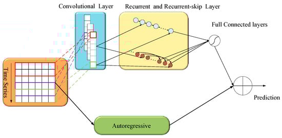
Figure 1.
LSTNet structure.
The individual modules of LSTNet are specified as follows.
- (1)
- Convolutional module
This layer is a convolutional neural network without pooling layers, and this structure extracts short-term features in the time dimension and local dependencies between variables. The convolution kernel performs the following convolutional operations on the input matrix.
where is the feature matrix obtained from the convolution operation, is the weight matrix, is the offset vector, and is the parameter obtained from the network learning, and is the Relu function.
- (2)
- Recurrent and Recurrent-skip modules
Recurrent-skip modules are RNN structures with time-hopping links and jumping links between the current unit and hidden units of the same phase in any adjacent recurrent unit to extend the time span of the information flow. The LSTM network is employed in this paper as a variant of RNN to serve as the recurrent unit. Basic units of the LSTM network consist of forgetting gates, input gates, and output gates. The structure of the recurrent-skip unit is shown in Figure 2.
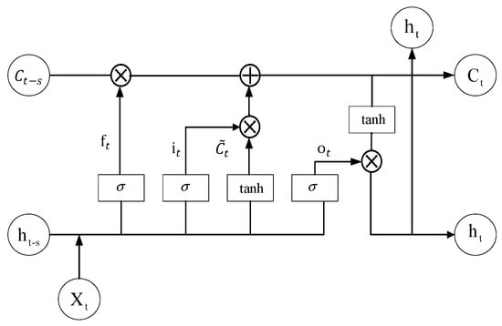
Figure 2.
LSTM structure.
The input in the forgetting gate, together with the state memory unit and the intermediate output , determines which information the state memory unit is to forget. The input is changed by the sigmoid and tanh functions to determine which information is retained in the state memory unit. The intermediate outputs are determined by the updated and . The computational equations for the recurrent module and the recurrent-skip module are expressed uniformly as follows:
where , , , , are the forgetting gates, input gates, output gates, intermediate outputs, and cell states, respectively. , , , are the weights corresponding to the different state gates. , , , are the offset terms of the different state gates, respectively. is the number of hidden cells skipped, and when the value is 1, it is a LSTM network.
- (3)
- Autoregressive module
In the LSTNet architecture, the autoregressive module uses the classical autoregressive AR model as the linear component, and the AR model can be expressed by the following equation:
where is the predicted AR component prediction, and is the coefficient of the model, and is the window size of the input matrix.
The final prediction result of LSTNet is obtained by integrating the prediction of the recurrent module and the prediction of the autoregressive module model .
2.3. LSTNet Quantile Regression
2.3.1. Linear Quantile Regression
The traditional least squares method is linear, and, therefore, provides inadequate coverage in the analysis of factors that could influence the response variable. Additionally, predicting outcomes in the power system involves a variety of complex factors, and mean regression often produces poor results with low prediction accuracy. To address these challenges, Koenker et al. introduced the concept of quantile regression in 1978. This approach retains the statistical information of both explanatory and response variables and resolves the problem of heteroskedasticity, which can limit the usefulness of the more common least squares method. Considering a response variable , influenced by k factors , then the quantile regression model is:
where is the conditional quantile of the response variable given by the explanatory variable , is the quantile point, and , is the regression coefficient vector. The regression coefficient vector changes with the quantile , which is significantly different from the constant vector in the mean regression.
The estimation of the parameter vector can be translated into solving the following optimization problem:
where is the sample size. Before optimizing the quantile regression, the test function is defined and the optimal parameters are optimally estimated by minimizing the test function, which is defined as:
is an indicative function and is calculated as:
After obtaining an estimate of the parameter vector , the conditional quantile at the quantile τ can be measured. When takes continuous values on the (0,1) interval, the conditional distribution of the response variable can be obtained.
2.3.2. Neural Network Quantile Regression
The quantile regression model is linear, which limits the ability to capture the complex patterns of influence between explanatory variables and the response variable that occur in more realistic behavior patterns. Nonlinear paradigms are a better fit for these behavior patterns. Artificial neural networks (ANNs) are well-suited for addressing these nonlinear paradigms, thanks to their ability to model nonlinear structures between inputs and outputs. To this end, Taylor introduced the neural network quantile regression model [16], which is presented below:
where is the vector of connection weights between the input layer and the implied layer, and is the vector of connection weights between the implied layer and the output layer. The estimation of the parameter vectors and can be transformed to solve the optimization problem as follows:
where , are penalty parameters to avoid the network structure from falling into an over-fitting state. After obtaining the parameter estimation vectors and , the conditional quantile estimates of can be obtained as:
when takes continuous values on the (0,1) interval, the conditional quantile curve is called the conditional distribution.
2.3.3. LSTNet Quantile Regression
LSTNet quantile regression consists of AR quantile regression, which is a linear quantile regression method in the autoregressive module of LSTNet, and LSTM quantile regression, which is a neural network quantile regression method in the recurrent module. According to conditional quantile theory, the quantile curve of is the distribution function when belongs to (0,1), and let (, , , ) be the mutually independent quantile functions obtained from the estimated probability distribution:
where ; equals the number of quartiles; is the quantile function; and is the conditional quantile of .
Due to the strong generalization ability of the kernel function, we applied it to construct probability density functions that have a significant effect on the distribution of the response variable and used the rule-of-thumb for the bandwidth selection, which further enhances the smoothness and continuity of the probability density curve by integrating the obtained quantile functions. Using the obtained quantile function as an input to the kernel density estimation, the kernel density is estimated as:
where is the window width; n is the number of samples; and () is a non-negative kernel function, which can generally be chosen as Gaussian, matrix, triangular, epanechnikov, etc. In this paper, we use the Gaussian function.
Different kernel function choices are not sensitive in kernel density estimations, and the Gaussian kernel function is selected in this paper. The selection of different bandwidths directly affects the fitting effect of the distribution. If too large, the estimated curve will be too smooth and the data structure will be masked. If too small, the estimated curve will be under-smoothed, resulting in excessive data noise. Therefore, the choice of window width is the most critical when fitting with nonparametric kernel density estimation.
In this paper, the classical method Rule-of-Thumb method is used to select the window width, and the obtained window width can be expressed as:
where is the sample standard deviation.
2.4. Evaluation Metrics
Probabilistic forecasting aims to maximize the sharpness of the predicted distribution, but with reliability in mind. Reliability refers to the uniform consistency between the prediction and observation of the distribution. Sharpness refers to how closely the predicted distribution covers the actual distribution. For interval forecasting methods, the most commonly used reliability and sharpness metrics are the prediction interval coverage (PICP) and the prediction interval average width (PINAW).
where is the number of points to be predicted, is a Boolean quantity, and , indicating that the actual value falls within the prediction interval under the given confidence, indicating that the actual value falls outside the prediction interval. is the forecast time interval and and are the upper and lower limits of the electricity price forecast.
However, there is a contradiction between a high confidence level and a narrow interval width. In the 2014 global energy forecasting competition, the pinball loss was used to evaluate the effectiveness of probabilistic forecasting, which can solve the contradiction between PICP and PINAW by considering the reliability index and the sharpness index together. The smaller the pinball loss is, the better the probabilistic forecasting effect is.
In this paper, the performance of the probabilistic forecasting is evaluated by the average pinball loss (AL).
3. Case Studies
This section is dedicated to validating the effectiveness of our proposed method for day-ahead electricity price forecasting. First, we present an overview of the Danish electricity market. Then, using the SHAP method, we assess each feature’s importance on electricity prices and select the feature set with a relatively higher impact on the prices. Furthermore, we provide specific examples of how the selected features impact the prices. Finally, in order to verify the validity of the proposed method, we conduct point forecasting and probabilistic forecasting, respectively. By comparing the performance of the proposed model in point forecasting and probabilistic forecasting, we demonstrate that probabilistic forecasting can effectively quantify the uncertainty of prediction while guaranteeing accuracy. In both point forecasting and probabilistic forecasting, the models using SHAP feature selection have obvious improvements compared with the original models, which proves the effectiveness of the SHAP feature selection. Comparing the accuracy of the benchmark models with the proposed model, the latter is obviously superior to the others, which proves the advantage of the LSTNet quantile regression.
3.1. Overview of the Danish Electricity Market
This paper uses the Danish electricity market dataset. Denmark is a pioneer country in green energy transition. According to statistics, fossil energy generation accounts for 25.9% of the Danish energy mix, while clean energy generation accounts for 74.1%. Among them, 50% of Denmark’s electricity consumption comes from wind and solar energy, while the proportion of coal generation is only 13%. The Danish Energy Agency estimates that Denmark’s green energy production will exceed the country’s total electricity consumption in 2028. The Danish grid is divided into two parts: the eastern grid (Zealand, DK2) and the western grid (Jutland and Funen, DK1), where the eastern grid DK2 is connected to Sweden AC to form the Nordic synchronous grid, and the western grid DK1 is connected to Germany AC to be part of the central European synchronous grid. In addition, the eastern grid is connected to the German DC and the western grid is connected to the Norwegian DC. Denmark’s eastern grid is connected to the western grid via a 400 kV DC line with a transmission capacity of 600,000 kW. the maximum export capacity of Denmark’s connection to neighboring countries is 6.52 million kW and the maximum import capacity is 5.73 million kW. The exchange of electricity between Denmark and neighboring countries depends mainly on tariff differences and transmission capacity limitations. For example, in 2015, Denmark imported large amounts of electricity from Norway and Sweden due to their high hydroelectric generation capacity and low electricity prices. The general situation of the Danish electricity market is shown in Figure 3.
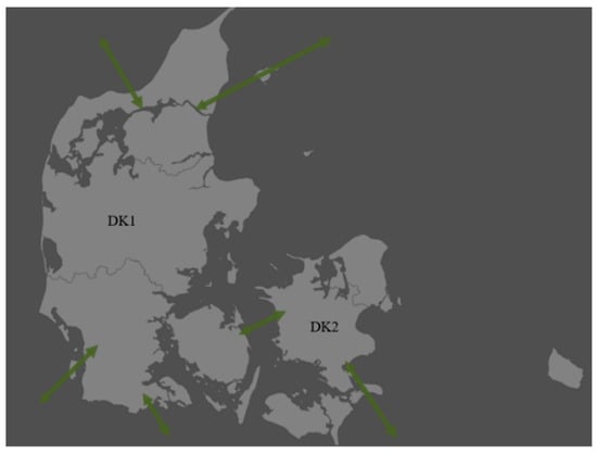
Figure 3.
Overview of the Danish electricity market.
All data in this paper are available from www.energidataservice.dk. The time span of the dataset is from 1 May 2019 to 31 August 2019. The day-ahead tariff for the DK1 region is the forecast tariff, as shown in Figure 4. The dataset contains features as shown in Table 1. The training set is from 1 May 2019 to 31 July 2019 and the test set is from 1 August 2019 to 31 August 2019.
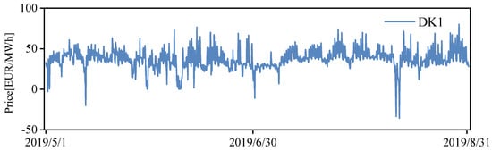
Figure 4.
Electricity price time series for DK1.

Table 1.
The features included.
3.2. Feature Selection and Analysis
In this paper, the SHAP method is used for feature selection of the dataset. The prediction model is LSTNet and the optimization algorithm is the adaptive moment estimation method (ADAM), which can design independent adaptive learning rates for different parameters, thus it is better suited for problems with non-smooth objectives, noisy, or sparse gradients. After hyperparameter adjustment, the number of neurons in the LSTNet model is 128 for RNN and RNN-skip, 64 for CNN, and 24 for the skip parameter.
Figure 5 shows the feature importance ranking chart similar to the traditional feature selection method. The traditional feature selection method usually compares feature series and tariff series and calculates the correlation coefficient between them, and this correlation coefficient is the importance of that class of features, such as the Pearson correlation coefficient. In contrast, the SHAP method characterizes the importance of each class of features by averaging the absolute values of the importance of individual features under each sample. It can be seen that the largest influence on the predicted electricity price is the feature DK2_7. Among the neighboring countries, the German electricity market has the largest influence on the Danish electricity market, with DE_1 ranked fourth in the feature importance ranking chart. Among all renewable energy sources, the feature HydroPower_1, which characterizes hydropower, is the most important, followed by the feature Wind_1, which characterizes wind power, and finally by the feature Solar_1, which characterizes photovoltaic power generation. Among all electric energy exchange features, the electric energy exchange feature ExGE_1 between the DK1 region and Germany is the most important, followed by the electric energy exchange feature ExGB_1 between the DK1 region and the DK2 region. Finally, among all the electrical energy exchange features, the electrical energy exchange feature ExGE_1 between DK1 region and Germany is the most important, followed by the electrical energy exchange feature ExGB_1 between DK1 region and DK2 region, and finally, the electrical energy exchange feature ExNO_1 between DK1 region and Norway. In this paper, we select the top seven features as the input feature set.
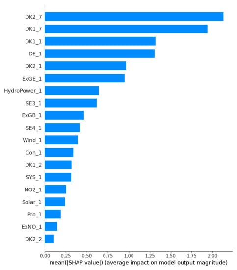
Figure 5.
Features rank.
Figure 6 shows the effect of each sample on the predicted electricity price under different features. Each point on each feature row represents a sample from the test set. The color of the points is determined by the value of the corresponding feature under that sample. DK2_7 represents the tariff in the DK2 region with a lag of one week from the forecast date. It can be seen that most of the blue sample points are in the left half of the region and most of the purple sample points are in the right half of the region. This means that the feature pulls down the forecasted electricity price when the price of electricity in the DK2 region one week before is lower, and conversely raises the forecasted electricity price when the price of electricity in the DK2 region one week before is higher. The case of feature DK1_7 is similar to that of feature DK2_7, except that the peak of importance of feature DK1_7 is greater. The case of feature SE4_1 is different from that of features DK1_7 and DK2_7. It can be seen that most of the blue sample points in this feature row are located in the right zone, while the purple sample points are located in the left half of the zone. This means that when predicting DK1 electricity prices, the feature will increase the predicted electricity prices when the electricity prices in the SE4 region are lower a day ago, and conversely the feature will pull down the predicted electricity prices when the electricity prices in the DK1 region are higher a day ago.
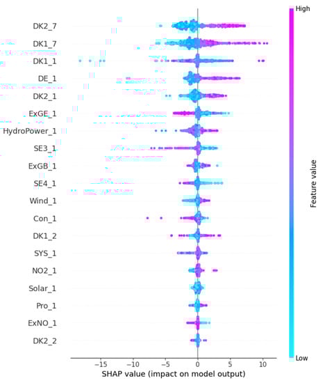
Figure 6.
Features impact.
In order to gain more insight and analyze the Danish electricity market, we plotted the feature dependence between the values of the features and the importance of the features. Figure 7 shows the feature dependence plot for the wind power feature Wind_1. The vertical axis is the SHAP value and the horizontal axis is wind power generation. It can be seen that when the wind power generation is less than 1000, the sample points are concentrated below the value of SHAP value 0. When the wind power generation is greater than 1000, the sample points are concentrated above the value 0. This means that for the Danish electricity market, the threshold value of wind power discharge affecting electricity price is 1000 a few days ago, and when the feature Wind_1 is less than 1000, the wind power feature reduces the electricity price; when the feature Wind_1 is greater than 1000, the wind power feature increases the electricity price.
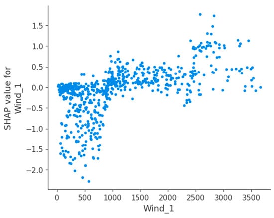
Figure 7.
SHAP dependence plot of the feature Wind_1.
Figure 8 shows the feature dependence diagram of the electric energy exchange feature ExGE_1. It can be seen that when the electric energy exchange between DK1 region and Germany is less than 800, the sample points are concentrated above the value of SHAP value 0. The sample points are concentrated below the value 0 when the electricity exchange is greater than 1000. This means that for the Danish electricity market, the threshold value of the electricity exchange between DK1 and Germany is 800, and when the feature ExGE_1 is less than 800, the electricity exchange feature increases the electricity price; when the feature ExGE_1 is greater than 800, the electricity exchange feature decreases the electricity price.
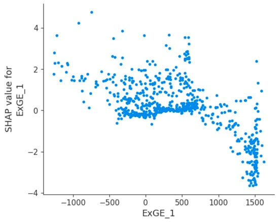
Figure 8.
SHAP dependence plot of the feature ExGE_1.
3.3. Probabilistic Forecasting Results
In this paper, we propose a probability density prediction method based on LSTNet quantile regression. After obtaining the predicted electricity prices under different quartiles, we use the kernel density estimation algorithm to estimate the probability density distribution of the predicted electricity prices and obtain the prediction intervals at different confidence levels. In this paper, we set LSTM and BPNN as the benchmark models and the inter-quantile quantile interval is 0.1.
It is worth mentioning that when the quantile is 0.5, the predicted price quantile is the point forecasting price. Table 2 shows the forecasts of different models when the quantile is 0.5. In this paper, we adopt RMSE and MAPE as the point prediction model evaluation metrics.
Table 2.
Point forecasting metrics.
It can be seen that among all neural network models, the LSTNet model has the best prediction performance and is most suitable for the day-ahead electricity price forecasting task. Specifically, among the models without feature selection, the LSTNet model has the smallest error metrics RMSE and MAPE; among the models with feature selection, the SHAP–LSTNet model has the smallest error metrics. Among them, compared with the LSTM model, the error metrics RMSE and MAPE of the LSTNet model reduce by 36.41% and 42.61%, respectively. Compared with the SHAP–BPNN model, the error metrics RMSE and MAPE of the SHAP–LSTNet model reduces by 44.96% and 47.87%, respectively. In the comparison between the model without feature selection and the model with feature selection, the error metrics of the model with feature selection are smaller. For example, the error metrics RMSE and MAPE of the SHAP–LSTNet model reduced by 52.62% and 35.76%, respectively, compared to the LSTNet model. This is mainly because feature selection reduces redundant features and reduces the risk of model overfitting.
Figure 9 shows the point forecast price for a three-day period in August 2019. It can be seen that the SHAP–LSTNet model fits the real electricity price curve best.
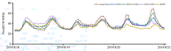
Figure 9.
Point forecasting results.
After obtaining different price quartiles, the kernel density estimation is used to obtain the probability density functions at different moments of the forecast day and the prediction intervals at different confidence levels. Table 3 shows the metrics at different confidence levels. The confidence levels are 0.9, 0.8, and 0.7, respectively.
Table 3.
Interval forecasting metrics.
It can be seen that the metrics at different confidence levels are different. For example, at the confidence level of 0.9, the largest PINAW among all models is the SHAP–LSTNet model, however, the smallest PICP is SHAP–BPNN. At this time, it is difficult to select the best model based on the PINAW and PICP alone, so we use the average pinball loss to assist us in our decision. At this point, the AL metrics of the SHAP–LSTNet and SHAP–BPNN models are 0.41 and 2.61, respectively, and it is clear that the former is more suitable for the day-ahead price forecasting task. Figure 10 shows the prediction interval of different models at the confidence level of 0.9. It can be seen that the narrowest interval width is the SHAP–BPNN model, but most of the actual price points are not covered in this interval, which is obviously not possible. The most desirable model is SHAP–LSTNet, which basically covers all actual price points except for a few, and the interval width is also relatively small.
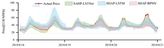
Figure 10.
Interval forecasting results of different models.
Moreover, from the table we can see that the PINAW is higher, but the PICP is larger at a high confidence level, and the PICP is smaller, but the PINAW is lower at a low confidence level. Figure 11 shows the prediction interval plot of the SHAP–LSTNet model at different confidence levels. It can be seen that the higher the confidence level, the more actual price points are covered by the prediction interval, but the larger the interval width, while the lower the confidence level, the smaller the interval width, but fewer actual price points are covered by the prediction interval. Similarly, we use the average pinball loss to complicate our decision. It can be seen that at all confidence levels, the 0.9 confidence level has the smallest AL indicator.
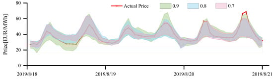
Figure 11.
Interval forecasting results at different confidence levels.
In summary, the best model is the SHAP–LSTNet model at a 0.9 confidence level.
4. Conclusions
In response to the uncertainties associated with renewable energy and the growing number of features in electricity price forecasting, this paper proposes a probabilistic method for predicting day-ahead electricity prices using SHAP feature selection and LSTNet quantile regression. In order to reduce redundant features and over-fitting, and improve forecasting performance, the SHAP method is utilized to handle the expanding set of input features that arise from an integrated market. Furthermore, we assess the importance and direction of the impact of features on electricity prices, which significantly improves the interpretability of forecasts. We also employ a probability forecasting method to quantify the uncertainty in electricity price forecasting. By applying the LSTNet quantile regression based on kernel density estimation, we can estimate the probability distribution of the predicted electricity prices and obtain the predicted electricity price interval to achieve conditional probability density prediction. Our results demonstrate the effectiveness of the proposed feature selection method at reducing overfitting and improving prediction accuracy. Moreover, the proposed method outperforms the comparison algorithm, and its prediction intervals effectively quantify the uncertainty in electricity price forecasting.
Author Contributions
Conceptualization, H.L. and X.S.; Data curation, H.L.; Formal analysis, H.L. and J.L.; Funding acquisition, X.S. and X.T.; Investigation, H.L. and X.T.; Methodology, H.L.; Project administration, X.S.; Resources, J.L.; Software, H.L. and X.S.; Supervision, X.S.; Validation, H.L. and X.S.; Visualization, H.L.; Writing—original draft preparation, H.L.; Writing—review and editing, X.S. All authors have read and agreed to the published version of the manuscript.
Funding
This research was granted by the National Natural Science Foundation of China under Grant U22B20123.
Data Availability Statement
Not applicable.
Conflicts of Interest
The authors declare no conflict of interest.
References
- Weron, R. Electricity price forecasting: A review of the state-of-the-art with a look into the future. Int. J. Forecast. 2014, 30, 1030–1081. [Google Scholar] [CrossRef]
- Nowotarski, J.; Weron, R. Recent advances in electricity price forecasting: A review of probabilistic forecasting. Renew. Sustain. Energy Rev. 2018, 81, 1548–1568. [Google Scholar] [CrossRef]
- Lago, J.; Marcjasz, G.; De Schutter, B.; Weron, R. Forecasting day-ahead electricity prices: A review of state-of-the-art algorithms, best practices and an open-access benchmark. Appl. Energy 2021, 293, 116983. [Google Scholar] [CrossRef]
- Dash, P.K.; Satpathy, H.P.; Liew, A.C.; Rahman, S. A real-time short-term load forecasting system using functional link network. IEEE Trans. Power Syst. 1997, 12, 675–680. [Google Scholar] [CrossRef]
- Conejo, A.; Plazas, M.; Espinola, R.; Molina, A. Day-Ahead Electricity Price Forecasting Using the Wavelet Transform and ARIMA Models. IEEE Trans. Power Syst. 2005, 20, 1035–1042. [Google Scholar] [CrossRef]
- Garcia, R.C.; Contreras, J.; Vanakkeren, M.; Garcia, J.B.C. A GARCH Forecasting Model to Predict Day-Ahead Electricity Prices. IEEE Trans. Power Syst. 2005, 20, 867–874. [Google Scholar] [CrossRef]
- Zhou, S.; Zhou, L.; Mao, M.; Tai, H.-M.; Wan, Y. An Optimized Heterogeneous Structure LSTM Network for Electricity Price Forecasting. IEEE Access 2019, 7, 108161–108173. [Google Scholar] [CrossRef]
- Shi, H.; Wang, L.; Scherer, R.; Wozniak, M.; Zhang, P.; Wei, W. Short-Term Load Forecasting Based on Adabelief Optimized Temporal Convolutional Network and Gated Recurrent Unit Hybrid Neural Network. IEEE Access 2021, 9, 66965–66981. [Google Scholar] [CrossRef]
- Chang, Z.; Zhang, Y.; Chen, W. Electricity price prediction based on hybrid model of adam optimized LSTM neural network and wavelet transform. Energy 2019, 187, 115804. [Google Scholar] [CrossRef]
- Wang, Z.; Qu, J.; Fang, X.; Li, H.; Zhong, T.; Ren, H. Prediction of early stabilization time of electrolytic capacitor based on ARIMA-Bi_LSTM hybrid model. Neurocomputing 2020, 403, 63–79. [Google Scholar] [CrossRef]
- Peng, L.; Liu, S.; Liu, R.; Wang, L. Effective long short-term memory with differential evolution algorithm for electricity price prediction. Energy 2018, 162, 1301–1314. [Google Scholar] [CrossRef]
- Xie, X.; Xu, W.; Tan, H. The Day-Ahead Electricity Price Forecasting Based on Stacked CNN and LSTM. Intell. Sci. Big Data Eng. 2018, 11266, 216–230. [Google Scholar] [CrossRef]
- Zahid, M.; Ahmed, F.; Javaid, N.; Abbasi, R.A.; Zainab Kazmi, H.S.; Javaid, A.; Bilal, M.; Akbar, M.; Ilahi, M. Electricity Price and Load Forecasting using Enhanced Convolutional Neural Network and Enhanced Support Vector Regression in Smart Grids. Electronics 2019, 8, 122. [Google Scholar] [CrossRef]
- Lai, G.; Chang, W.-C.; Yang, Y.; Liu, H. Modeling Long- and Short-Term Temporal Patterns with Deep Neural Networks. In Proceedings of the SIGIR ‘18: The 41st International ACM SIGIR Conference on Research & Development in Information Retrieval, Ann Arbor, MI, USA, 8–12 July 2018; pp. 95–104. [Google Scholar] [CrossRef]
- Zhao, C.; Wan, C.; Song, Y. Operating Reserve Quantification Using Prediction Intervals of Wind Power: An Integrated Probabilistic Forecasting and Decision Methodology. IEEE Trans. Power Syst. 2021, 36, 3701–3714. [Google Scholar] [CrossRef]
- Doherty, R.; O’Malley, M. A New Approach to Quantify Reserve Demand in Systems with Significant Installed Wind Capacity. IEEE Trans. Power Syst. 2005, 20, 587–595. [Google Scholar] [CrossRef]
- Bludszuweit, H.; Dominguez-Navarro, J.A.; Llombart, A. Statistical Analysis of Wind Power Forecast Error. IEEE Trans. Power Syst. 2008, 23, 983–991. [Google Scholar] [CrossRef]
- Baharvandi, A.; Aghaei, J.; Niknam, T.; Shafie-Khah, M.; Godina, R.; Catalao, J.P.S. Bundled Generation and Transmission Planning Under Demand and Wind Generation Uncertainty Based on a Combination of Robust and Stochastic Optimization. IEEE Trans. Sustain. Energy 2018, 9, 1477–1486. [Google Scholar] [CrossRef]
- Shi, J.; Ding, Z.; Lee, W.-J.; Yang, Y.; Liu, Y.; Zhang, M. Hybrid Forecasting Model for Very-Short Term Wind Power Forecasting Based on Grey Relational Analysis and Wind Speed Distribution Features. IEEE Trans. Smart Grid 2014, 5, 521–526. [Google Scholar] [CrossRef]
- Ma, X.-Y.; Sun, Y.-Z.; Fang, H.-L. Scenario Generation of Wind Power Based on Statistical Uncertainty and Variability. IEEE Trans. Sustain. Energy 2013, 4, 894–904. [Google Scholar] [CrossRef]
- Zhao, C.; Wan, C.; Song, Y. An Adaptive Bilevel Programming Model for Nonparametric Prediction Intervals of Wind Power Generation. IEEE Trans. Power Syst. 2020, 35, 424–439. [Google Scholar] [CrossRef]
- Wan, C.; Xu, Z.; Pinson, P.; Dong, Z.Y.; Wong, K.P. Optimal Prediction Intervals of Wind Power Generation. IEEE Trans. Power Syst. 2014, 29, 1166–1174. [Google Scholar] [CrossRef]
- Wan, C.; Cao, Z.; Lee, W.-J.; Song, Y.; Ju, P. An Adaptive Ensemble Data Driven Approach for Nonparametric Probabilistic Forecasting of Electricity Load. IEEE Trans. Smart Grid 2021, 12, 5396–5408. [Google Scholar] [CrossRef]
- Wan, C.; Wang, J.; Lin, J.; Song, Y.; Dong, Z.Y. Nonparametric Prediction Intervals of Wind Power via Linear Programming. IEEE Trans. Power Syst. 2018, 33, 1074–1076. [Google Scholar] [CrossRef]
- Shi, Y.; Chen, N. Conditional Kernel Density Estimation Considering Autocorrelation for Renewable Energy Probabilistic Modeling. IEEE Trans. Power Syst. 2021, 36, 2957–2965. [Google Scholar] [CrossRef]
- Khorramdel, B.; Chung, C.Y.; Safari, N.; Price, G.C.D. A Fuzzy Adaptive Probabilistic Wind Power Prediction Framework Using Diffusion Kernel Density Estimators. IEEE Trans. Power Syst. 2018, 33, 7109–7121. [Google Scholar] [CrossRef]
- Zhang, H.; Liu, Y.; Yan, J.; Han, S.; Li, L.; Long, Q. Improved Deep Mixture Density Network for Regional Wind Power Probabilistic Forecasting. IEEE Trans. Power Syst. 2020, 35, 2549–2560. [Google Scholar] [CrossRef]
- Wan, C.; Zhao, C.; Song, Y. Chance Constrained Extreme Learning Machine for Nonparametric Prediction Intervals of Wind Power Generation. IEEE Trans. Power Syst. 2020, 35, 3869–3884. [Google Scholar] [CrossRef]
- Wan, C.; Lin, J.; Song, Y.; Xu, Z.; Yang, G. Probabilistic Forecasting of Photovoltaic Generation: An Efficient Statistical Approach. IEEE Trans. Power Syst. 2017, 32, 2471–2472. [Google Scholar] [CrossRef]
- Wan, C.; Lin, J.; Wang, J.; Song, Y.; Dong, Z.Y. Direct Quantile Regression for Nonparametric Probabilistic Forecasting of Wind Power Generation. IEEE Trans. Power Syst. 2017, 32, 2767–2778. [Google Scholar] [CrossRef]
- Torregrossa, D.; Le Boudec, J.-Y.; Paolone, M. Model-free computation of ultra-short-term prediction intervals of solar irradiance. Sol. Energy 2016, 124, 57–67. [Google Scholar] [CrossRef]
- Wan, C.; Lin, J.; Guo, W.; Song, Y. Maximum Uncertainty Boundary of Volatile Distributed Generation in Active Distribution Network. IEEE Trans. Smart Grid 2018, 9, 2930–2942. [Google Scholar] [CrossRef]


Disclaimer/Publisher’s Note: The statements, opinions and data contained in all publications are solely those of the individual author(s) and contributor(s) and not of MDPI and/or the editor(s). MDPI and/or the editor(s) disclaim responsibility for any injury to people or property resulting from any ideas, methods, instructions or products referred to in the content. |
© 2023 by the authors. Licensee MDPI, Basel, Switzerland. This article is an open access article distributed under the terms and conditions of the Creative Commons Attribution (CC BY) license (https://creativecommons.org/licenses/by/4.0/).