Article

Microgrid Protection Coordination Considering Clustering and Metaheuristic Optimization

by
Javier E. Santos-Ramos
1,
Sergio D. Saldarriaga-Zuluaga
2,
Jesús M. López-Lezama
1,*,
Nicolás Muñoz-Galeano
1 and
Walter M. Villa-Acevedo
1
1
Research Group on Efficient Energy Management (GIMEL), Department of Electrical Engineering, Universidad de Antioquia (UdeA), Medellín 050010, Colombia
2
Facultad de Ingenieria, Departamento de Eléctrica, Institución Universitaria Pascual Bravo, Medellín 050036, Colombia
*
Author to whom correspondence should be addressed.
Energies 2024, 17(1), 210; https://doi.org/10.3390/en17010210
Submission received: 28 November 2023 / Revised: 24 December 2023 / Accepted: 28 December 2023 / Published: 30 December 2023
(This article belongs to the Section A1: Smart Grids and Microgrids)

Abstract

:
This paper addresses the protection coordination problem of microgrids combining unsupervised learning techniques, metaheuristic optimization and non-standard characteristics of directional over-current relays (DOCRs). Microgrids may operate under different topologies or operative scenarios. In this case, clustering techniques such as K-means, balanced iterative reducing and clustering using hierarchies (BIRCH), Gaussian mixture, and hierarchical clustering were implemented to classify the operational scenarios of the microgrid. Such scenarios were previously defined according to the type of generation in operation and the topology of the network. Then, four metaheuristic techniques, namely, Genetic Algorithm (GA), Particle Swarm Optimization (PSO), Invasive Weed Optimization (IWO), and Artificial Bee Colony (ABC) were used to solve the coordination problem of every cluster of operative scenarios. Furthermore, non-standard characteristics of DOCRs were also used. The number of clusters was limited to the maximum number of setting setting groups within commercial DOCRs. In the optimization model, each relay is evaluated based on three optimization variables, namely: time multiplier setting (TMS), the upper limit of the plug setting multiplier (PSM), and the standard characteristic curve (SCC). The effectiveness of the proposed approach is demonstrated through various tests conducted on a benchmark test microgrid.

1. Introduction

Microgrids are decentralized and self-sustaining energy systems that integrate renewable sources, storage, and traditional power generation for providing reliable and resilient energy supply to localized loads [1]. Microgrids can operate independently or in coordination with the main power grid and under several topologies, therefore offering numerous operational scenarios. They enhance energy resilience by providing a backup power source during grid outages, reduce greenhouse gas emissions by utilizing clean energy sources, and promote energy independence by reducing reliance on centralized fossil fuel-based power generation [2,3,4]. Furthermore, microgrids empower local communities and businesses to take control of their energy supply, fostering a more sustainable and resilient energy future.
In the broader context of the energy transition, microgrids are instrumental in achieving the goals of decarbonization, decentralization, and democratization of energy. Decarbonization involves reducing the carbon footprint of the energy sector by shifting towards cleaner and renewable energy sources. Microgrids enable this transition by facilitating the integration of sustainable energy resources at the local level [5,6,7,8]. Decentralization involves moving away from a highly centralized energy system dominated by a few large power plants towards a more distributed model [9,10,11]. Finally, democratization signifies greater inclusivity and involvement in energy decisions as can be achieved through the creation of energy communities. Microgrids empower users to participate actively in energy production and management, giving them a stake in the energy transition and promoting a more equitable and sustainable energy future [12,13].
While microgrids present numerous advantages, they face challenges in terms of integration with the main grid while ensuring reliability and resilience. This requires addressing technical issues to ensure a smooth connection and disconnection from the main grid, avoiding disruptions or safety concerns. Additionally, ensuring uninterrupted power supply to critical facilities during grid outages requires robust design, adequate maintenance, and proper coordination of the protection scheme. The focus of this paper is on a complete protection coordination of microgrids considering clustering and metaheuristic optimization [12,13,14,15,16,17,18,19,20].
Effective protection coordination is crucial for ensuring the safety and reliability of microgrid systems. Microgrids, often incorporating various distributed energy resources, require a hierarchical setup of protective devices and settings to quickly detect and isolate faults, preventing equipment damage and electrical hazards. Protection coordination enhances overall system reliability and ensures the safety of personnel and equipment, making it an essential aspect of microgrid design and operation. The challenges in coordinating protections arise from the inclusion of distributed generation (DG) units that introduce bidirectional power flows, variations in impedance, low short-circuit currents, fluctuations in fault currents, and changes in network topology. Traditional protection devices, such as overcurrent relays, may experience reduced sensitivity, selectivity, and response speed in the presence of these factors [21].
Various researchers have proposed innovative solutions to address protection coordination challenges. In [14], a Protection Coordination Index (PCI) was formulated to evaluate the effects of DG on protection coordination in distribution networks. Other studies, such as [15,16,17], employ strategies based on reverse time characteristics, optimization, and evolutionary algorithms to achieve effective protection coordination. Protection coordination in microgrids often involves the use of directional over-current relays (DOCRs), a widely adopted solution in conventional distribution networks. However, the application of overcurrent relay-based protection schemes becomes complex in microgrids, due to the challenges mentioned earlier. Researchers have explored various optimization techniques to address this complexity, such as linear programming [16], evolutionary algorithms [22,23,24], and modified metaheuristic algorithms [18]. These approaches aim to optimize relay settings to minimize system disruption during faults while adhering to coordination constraints. Furthermore, the incorporation of non-standard characteristics in protection coordination has gained attention. In [19], a comprehensive classification and analysis of non-standard characteristics was conducted to identify the advantages and disadvantages in the context of protection coordination. Recommendations for future research in this field were provided, outlining essential requirements for designing non-standard features in relays to improve coordination in microgrids.
The methodology proposed in this paper integrates a set of advanced strategies. Unsupervised learning techniques are used to classify different operational scenarios in a specific network. Additionally, non-standard features are used in formulating the protection coordination problem. The solution to this problem, as well as the determination of the optimal configuration for each relay, is carried out using metaheuristic techniques. In Table 1, papers addressing the aforementioned topics are presented, and the knowledge gap covered in this paper is identified. In [17,18,22,23,24], the protection coordination problem is solved using metaheuristic techniques; nonetheless, there is no classification of operational scenarios or the use of non-standard characteristics. On the other hand, researchers in [20,21,25,26,27] address the coordination of protection problem using non-standard features and solve it with metaheuristic techniques. Finally, [28] uses unsupervised learning techniques to classify operational scenarios and solve the coordination problem through linear programming, while [29,30] combine unsupervised learning techniques with metaheuristic techniques to address the coordination problem.
The main motivation of this paper is to complement and expand previous research work on microgrids protection coordination. In particular, the main challenge addressed in this research is the comprehensive integration of unsupervised machine learning techniques, metaheuristic approaches, and non-standard characteristics in microgrid protection coordination. These aspects have not been covered in previous research work, and constitute the research’s main contribution.
The contribution of this paper lies in expanding the research carried out in [21,25,26,30]. Previous analyses conducted in [21,25,26] use non-standard features to pose the coordination challenge, as well as metaheuristic techniques to solve it; however, they do not incorporate clustering techniques to classify operational scenarios into groups of overcurrent relay configurations. On the other hand, [30] employs clustering techniques and metaheuristic methods, although it does not make use of non-standard features. To summarize, the main features and contributions of this paper are as follows:
  • Unsupervised machine learning techniques, metaheuristic techniques and non-standard characteristics of DOCRs are integrated into a single methodology to solve the protection coordination problem of microgrids that operate under several operational scenarios.
  • Unsupervised machine learning techniques are implemented to cluster the microgrid’s set of operative scenarios (limited to the maximum number of configuration groups in commercially available relays).
  • Four metaheuristic techniques, namely GA, PSO, IWO, and ABC, are implemented to solve the optimal protection coordination of every cluster identified by the unsupervised machine learning techniques.
  • Non-standard characteristics of DOCRs are introduced in the protection coordination study. These correspond to considering the maximum limit of the Plug Setting Multiplier (PSM) as a decision variable and selecting from different types of relay operating curves.
This paper is organized as follows: Section 2 addresses the mathematical formulation of the protection coordination problem as a mixed-integer nonlinear programming problem. Section 3 presents the methodology along with a brief description of unsupervised machine learning algorithms and the metaheuristic techniques. Section 4 details the obtained results. Finally, Section 5 presents the conclusions of the research.

2. Mathematical Formulation

Protection coordination aims to ensure the reliability and safety of the electrical network by coordinating the operation of protective devices. This involves analyzing the time-current characteristics of these elements to selectively isolate faulty sections while maintaining power to the rest of the system. The relay’s response time is given by its characteristic curve. The characteristic curve of a relay represents its operating behavior and is a graphical representation of the relationship between the input signal or measured quantity and the relay’s response or output [21].
Equation (1) represents a general expression commonly found in the IEC [32] and IEEE [33] standards for the characteristic curve of a relay. The term P S M i f (plug setting multiplier) in Equation (2) describes the relationship between the fault current of relay i ( I f i ) and the pickup current of such relay ( i p i c k u p i ). In Equation (1), the expressions in the numerator and denominator of the first term are nonlinear. In the numerator, two variables, namely, the time multiplying setting of relay i ( T M S i ) and A, are multiplied. This last one is a variable that takes different values depending on the type of curve. On the other hand, in the denominator, there is a variable that depends on the reciprocal (inverse) of the pickup current raised to an unknown parameter B that depends on the type of curve selected. Finally, C is a parameter of the curve that is often used in IEEE standard. Note that distinct values of A, B, and C indicate different types of relay curves.
t i f = A T M S i P S M i f B 1 + C
P S M i f = I f i i p i c k u p i

2.1. Objective Function

Equation (3) represents the objective function, which seeks to minimize the aggregate operational time of DOCRs over a set of pre-defined faults. In this case, i and f are indexes representing relays and faults, respectively. Therefore, t i f is the operational time of relay i when fault f takes place. Also, m and n are quantities of relays and faults, respectively.
M i n i = 1 m f = 1 n t i f

2.2. Constraints

The objective function given by Equation (3) is subject to a set of constraints indicated in Equations (4)–(10). Equation (4) specifies the maximum and minimum values for the operating times of relay i. The constraint indicated by Equation (5) is commonly referred to as the coordination criterion. This means that for a given fault f the primary relay (denoted as i) must act before the backup relay (denoted as j). In this case, t i f and t j f indicate, respectively, the operation time of the main and backup relay for a fault f. Typical values of the Coordination Time Interval ( C T I ) are between 0.2 and 0.5 s. The limits of T M S i and i p i c k u p i are given by Equations (6) and (7), respectively. In this case, T M S i m i n and T M S i m a x are, respectively, the minimum and maximum allowed limits of T M S for relay i; while i p i c k u p i m i n and i p i c k u p i m a x are the minimum and maximum limits for i p i c k u p of relay i, respectively. In this case, T M S is a variable that must be determined within the coordination. In this paper, the upper limit of P S M is a non-standard characteristic which is introduced as a variable [21]. The minimum and maximum limits of P S M are denoted as P S M i m i n and P S M i m a x , respectively. The parameter P S M m a x allows for converting the inverse-time curve to definite-time depending on its value. Usually, these limits are considered as parameters; nonetheless, P S M i m a x is considered as a decision variable ranging between α and β as indicated in Equation (9). In this case, α and β were set to 5 and 100, respectively, based on [25].
Equation (10) indicates that is possible to choose from a set of relay curves. In this case, S C C i represents the standard curve of relay i, and Ω c is a set containing IEC [32] and IEEE [33] standard characteristic curves.
t i m i n t i f t i m a x
t j f t i f C T I
T M S i m i n T M S i T M S i m a x
i p i c k u p i m i n i p i c k u p i i p i c k u p i m a x
P S M i m i n P S M i P S M i m a x
α P S M i m a x β
S C C i Ω c

2.3. Codification of Candidate Solutions

Codification of candidate solutions is a key aspect when implementing metaheuristic optimization techniques. In this case, every DOCR features the ability to modify three parameters in their settings: the T M S , the operating curve ( S C C ) and the P S M m a x . Figure 1 illustrates the representation of a candidate solution for a system containing four relays. Each relay is associated with a set of three values, representing the three adjustable parameters, resulting in a candidate solution vector with a length of three times the number of relays of the system under study. The configuration for relay 1 would be as follows: set the T M S to 0.5, employ an I E C S I curve, and establish a maximum P M S m a x of 5; specific adjustments for the remaining relays are also depicted in a similar way.
It is worth mentioning that classic DOCR protection coordination models often used the TMS as the main optimization variable [18,34,35]. Nonetheless, multiple optimization variables are explored in [21,25,26,30] to improve the protection coordination times at the expense of more complicated mathematical modeling. In line with these research works, this paper uses three optimization variables for each relay.

3. Methodology

An IEC test network is used to carry out a series of simulations aimed at its characterization. This network has the particularity of being completely configurable, allowing the creation of several operative scenarios. In each of these scenarios, faults are deliberately introduced at different points in order to obtain the corresponding fault currents seen from each of the overcurrent relays. Although we used a specific microgrid text network, the proposed methodology can be applied to any network that has DOCRs; nonetheless, it should be adjusted for each particular case because each network may present different operational scenarios.
Each relay can be adjusted in four setting groups, which implies that each scenario can be categorized into four different groups, given the evaluation of their respective fault currents. This grouping task is carried out using unsupervised machine learning algorithms, configured with the objective of generating four clusters of the operating scenarios under consideration.
Once the clusters are established by means of each automatic learning algorithm, the optimal adjustment for each of the relays is determined using several metaheuristic techniques. This adjustment is calculated, aiming at minimizing the operation time of all the relays as indicated by the objective function described in Equation (3) and taking into account the constraints indicated by Equations (5)–(10).
Finally, the performance of the four clusters obtained by each machine learning approach and metaheuristic technique are compared, to determine which one ensures the minimum relay operation time, offers system selectivity (does not violate any model constraint) and requires the lowest computational cost (shortest simulation time). Figure 2 illustrates the flowchart of the implemented methodology.
It is worth mentioning that the proposed methodology is not limited to a given number of scenarios. In this sense, if there are new operational scenarios, they can be integrated without major modifications. On the other hand, the number of clusters and inclusion of non-standard features are limited to the specific characteristics of the relays.

3.1. Unsupervised Learning Techniques

This section describes a variety of unsupervised machine learning techniques that are used in the analysis and interpretation of complex data. Unlike supervised learning, where models are trained on labeled data, unsupervised learning addresses problems where labels are not available. These algorithms have the ability to cluster, classify and label data within sets without external guidance. In short, in unsupervised machine learning, no predefined labels are provided to the algorithm, allowing it to identify structures in the data on its own. This approach implies that an artificial intelligence system can group unclassified information according to similarities and differences, even if no categories have been previously defined. The fundamental goal of unsupervised learning is to discover hidden and meaningful patterns in unlabeled data [36]. By using algorithms such as hierarchical clustering, K-means, Gaussian mixtures, BIRCH, the data can be divided into meaningful clusters that share similar characteristics [37].

3.1.1. K-Means Algorithm

K-means is one of the most widely used clustering algorithms in the field of data mining. Its primary objective is to identify a partition within a dataset, forming distinct groups, each represented by a centroid. The user determines the number of clusters in advance. The underlying logic of K-means involves iteratively adjusting the positions of the centroids to achieve an optimal partitioning of the objects. In other words, the goal is to identify groups that bring together individuals with significant similarities to each other [38].
In order to measure the distance between two individual objects and determine which are more similar, the K-means algorithm uses distance functions. Within these functions, the Euclidean distance is one of the most commonly used, which is a measure of the smallest distance between two points, as shown in Equation (11). Figure 3 presents a flowchart illustrating the steps followed by the K-means algorithm for cluster classification.
d ( x , y ) = i = 1 n ( x i y i ) 2
Two variants of the K-means algorithm were considered: the mini-batch K-means algorithm and the K-means bisecting algorithm. The main objective of the mini-batch K-means clustering algorithm is to reduce the computation time when working with large data sets. This is done by using mini-batches as input, which are random subsets of the entire data set [39]. This approach uses small random batches of examples of a fixed size that can be stored in memory. At each iteration, a new random sample is selected from the data set and used to update the clusters, repeating this process until convergence is reached. Each mini-batch updates the clusters using a convex combination of the prototype and example values, applying a learning rate that decreases as the number of iterations increases. This learning rate is inversely proportional to the number of examples assigned to a cluster during the process. As more iterations are performed, the impact of new examples is reduced, so convergence can be determined when there are no changes in the groups for several consecutive iterations [40].
The K-means bisecting algorithm is a variant of the K-means algorithm used to perform divisive hierarchical clustering. K-means bisection is a method that combines features of divisive hierarchical clustering and K-means clustering. Unlike the traditional approach of dividing the data set into K groups at each iteration, the K-means bisection algorithm divides a group into two subgroups at each bisection step using K-means. This process is repeated until k groups are obtained [41].

3.1.2. Balanced Iterative Reducing and Clustering Using Hierarchies (BIRCH)

The BIRCH algorithm is a hierarchical clustering method designed for large datasets with a focus on memory efficiency. BIRCH constructs a tree-like data structure called a Clustering Feature Tree (CF Tree) by recursively partitioning data into subclusters using compact summary structures termed Cluster Feature (CF) entries. CF entries store statistical information of the subclusters, enabling BIRCH to efficiently update and merge clusters as new data points are introduced. For a set of data points X i in a cluster of N points in d dimensions ( X i = 1 , 2 , 3 , , N ), the clustering feature vector is defined as indicated in Equations (12)–(14), where N represents the number of points in the cluster; L S describes the linear sum of N points, and S S represents the sum of squares of the data points.
C F = ( N , L S , S S )
L S = i = 1 N X i
S S = i = 1 N ( X i ) 2
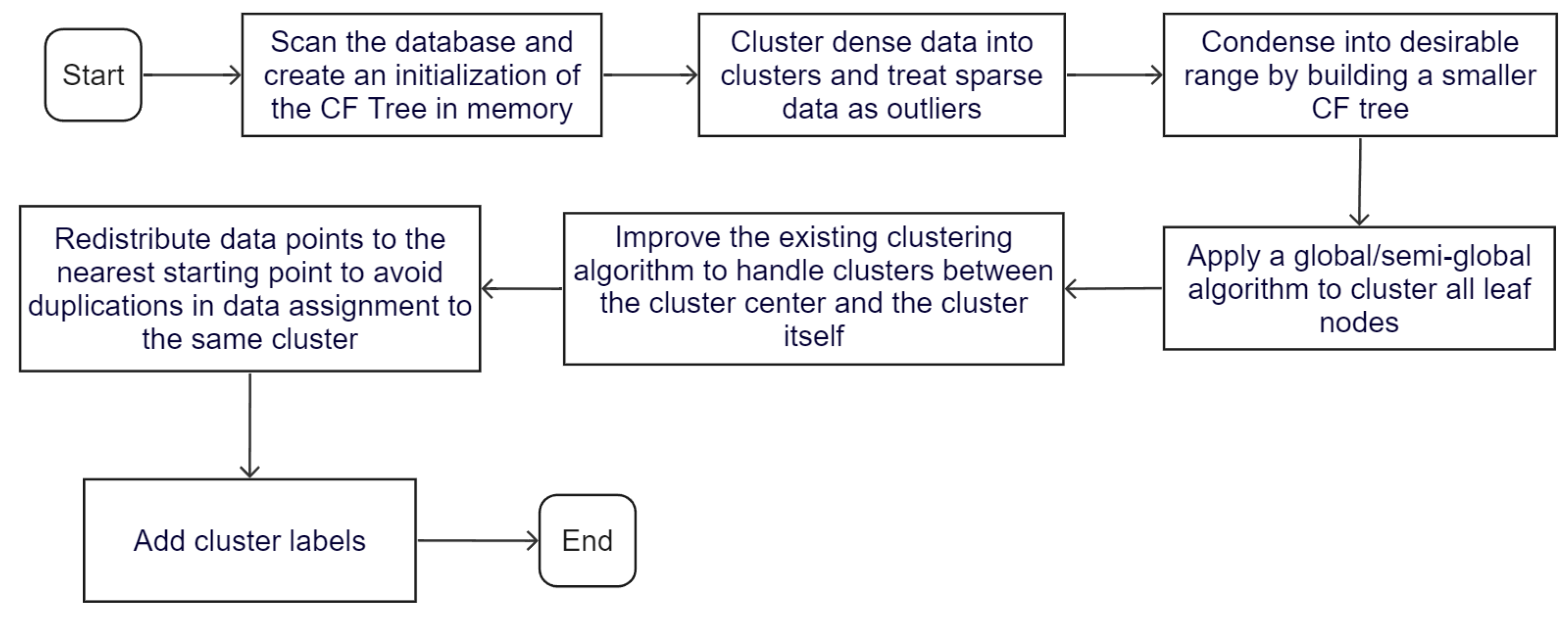
The BIRCH algorithm consists of four stages. In the first step, BIRCH scans the entire dataset, summarizing the information into CF trees. The second stage is the CF tree construction. In this case, the CF entries obtained from the initial scan are structured into a hierarchical CF Tree. The CF Tree maintains information about clusters at different levels of granularity, providing a scalable approach for handling large datasets. In the third stage, BIRCH performs clustering by navigating the CF Tree. It uses an agglomerative hierarchical clustering technique to merge clusters at various levels of the CF Tree based on certain thresholds, such as distance or the number of data points. In the final stage, BIRCH performs further refinement steps to enhance the quality of the clusters.
Since the leaf nodes of the CF Tree may not naturally represent the clustering results, it is necessary to use a clustering algorithm of global nature on the leaf nodes to improve the clustering quality [42]. The flowchart of the BIRCH algorithm is illustrated in Figure 4.

3.1.3. Gaussian Mixtures

A Gaussian Mixture Model (GMM) is defined as a parametric probability density function that is expressed as a weighted sum of Gaussian component densities [43]. The Gaussian distribution, also known as the normal distribution, is a continuous probability distribution defined by Equation (15):
N ( X | μ , M ) = 1 ( 2 π ) D 2 M e x p ( X μ ) T M 1 ( X μ ) 2
where μ is a D-dimensional mean vector, M is a D × D covariance matrix, which describes the shape of the Gaussian distribution, and | M | represents the determinant of M.
The Gaussian distribution has symmetry around the mean and is characterized by the mean and standard deviation. However, the unimodal property of a single Gaussian distribution cannot adequately represent the multiple density regions present in multimodal data sets encountered in practical situations.
A GMM is an unsupervised clustering technique that creates ellipsoid-shaped clusters based on probability density estimates using the Expectation-Maximization algorithm. Each cluster is modeled as a Gaussian distribution. The key difference from K-Means is that GMMs consider both mean and covariance, which provides a more accurate quantitative measure of fitness as a function of the number of clusters.
A GMM is represented as a linear combination of the basic Gaussian probability distribution and is expressed as shown in Equation (16):
p ( X ) = k = 1 K N ( X | μ k , M k )
where K represents the number of components in the mixture model, and p i k is known as the mixing coefficient, which provides an estimate of the density of each Gaussian component. The Gaussian density, represented by N ( X | m u k , M k ) , is referred to as the component of the mixture model. Each component k is described by a Gaussian distribution with mean μ k , covariance M k and mixing coefficient π k [44]. The flowchart of the Gaussian mixtures algorithm is illustrated in Figure 5.

3.1.4. Hierarchical Clustering Algorithms

Hierarchical clustering methods enable the identification of similar data groups based on their characteristics, using a similarity matrix. Discovering the hierarchical arrangement involves measuring the distance between every pair of data points and subsequently merging pairs based on these distances. Hierarchical algorithms construct groups from the bottom upwards, where each data point initially forms its own individual group. As the process continues, the two most alike groups are progressively combined into larger groups until eventually, all samples belong to a single comprehensive group.
The choice of distance metric (Euclidean, Manhattan, etc.) and linkage criterion (how distances between clusters are computed) greatly influences the results of hierarchical clustering. The linkage criterion determines which distance measure will be used between sets of observations when merging clusters. The algorithm will seek to combine pairs of clusters that minimize this criterion [45]. There are several available options:
  • Ward: seeks to minimize the variance of the merging groups.
  • Average: uses the average of the distances between each observation in the two sets.
  • Complete: is based on the maximum distances between all the observations in the two sets.
  • Single: uses the minimum of the distances between all the observations of the two sets of observations.
In addition to the linkage criterion, there is the Affinity criterion, which is a function that specifies the metric to be used to calculate the distance between instances in a feature matrix. The following distances were considered in the study [46,47]. Their mathematical expressions can be consulted in Appendix A.
  • Minkowski distance;
  • Standardized Euclidean distance;
  • Squared Euclidean distance;
  • Cosine distance;
  • Correlation distance;
  • Hamming distance;
  • Jaccard–Needham dissimilarity;
  • Kulczynski dissimilarity;
  • Chebyshev distance;
  • Canberra distance;
  • Bray–Curtis distance;
  • Mahalanobis distance;
  • Yule dissimilarity;
  • Dice dissimilarity;
  • Rogers–Tanimoto dissimilarity;
  • Russell–Rao dissimilarity;
  • Sokal–Michener dissimilarity;
  • Sokal–Sneath dissimilarity.

3.2. Implemented Metaheuristic Techniques

3.2.1. Genetic Algorithm (GA)

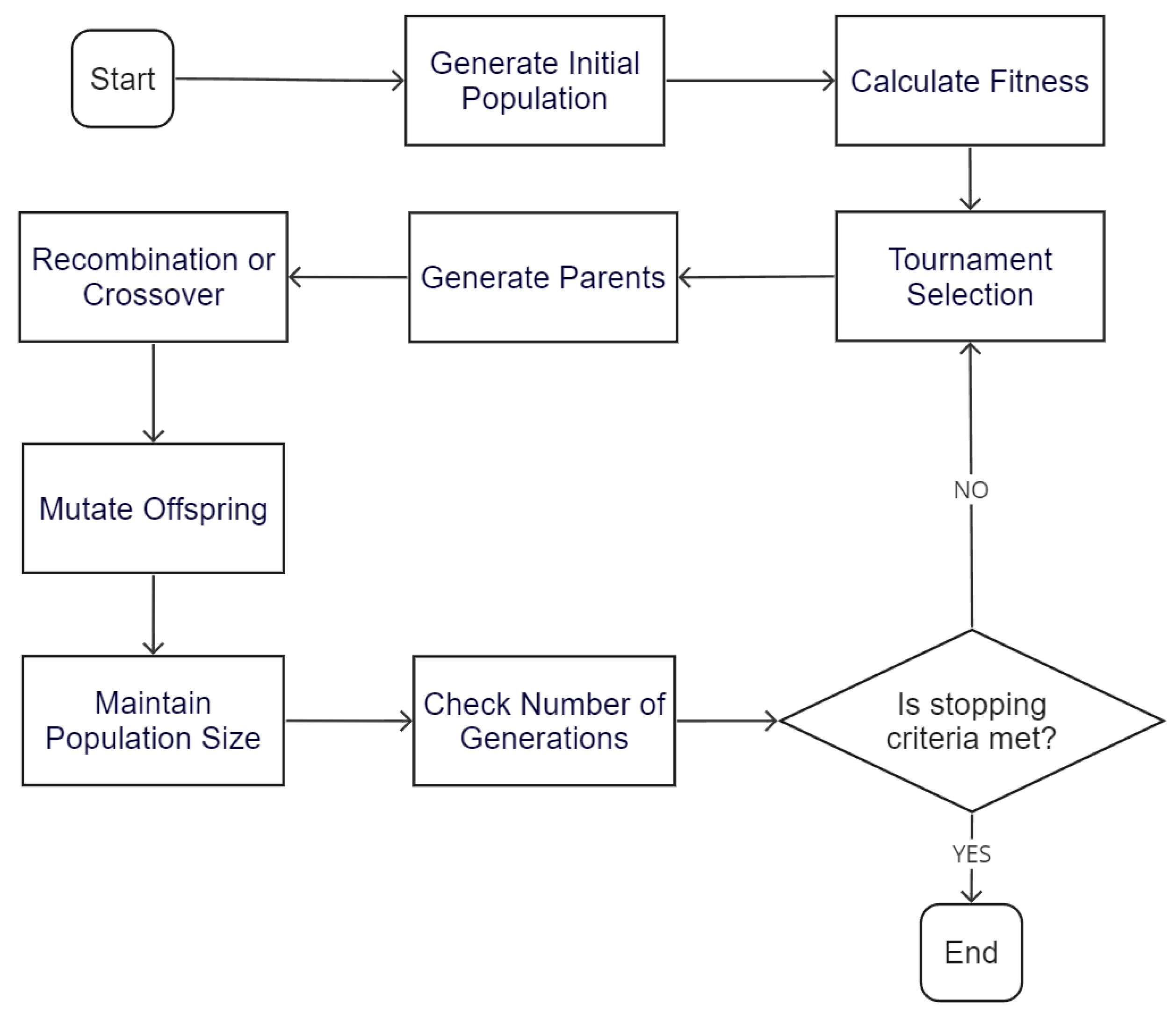
Genetic algorithms are optimization techniques inspired by the principle of natural selection. A GA emulates the process of natural selection by evolving a population of potential solutions through processes of selection, crossover, and mutation. Figure 6 illustrates the flowchart of the implemented GA.
Initially, a population is randomly generated where each element symbolizes a potential solution represented by an array. After setting up this initial population, the fitness of each candidate solution is calculated. Subsequently, a tournament selection process takes place within the current population, where a set number of individuals is randomly picked, and the best among them becomes a parent. This process is repeated to create pairs of parents, producing two new offspring through recombination or crossover. These offspring then undergo a mutation stage, introducing slight random alterations to prevent the algorithm from getting stuck in local optimal solutions. Throughout each generation, the fittest candidate solutions are chosen to replace lower-quality individuals, maintaining a constant population size until a specified number of generations is achieved.

3.2.2. Particle Swarm Optimization (PSO)

PSO is a stochastic method used to tackle combinatorial problems by employing a group of candidate solutions or particles that navigate through a search space based on rules governing their position and speed. Every particle’s trajectory is shaped by its own locally known best position and is directed towards the overall best positions discovered in the entire search space. The implementation steps of PSO are depicted in Figure 7. This approach starts by randomly generating potential solutions placed within the search space. Each potential solution includes two vectors: one defining its position and the other representing its velocity. These vectors are then adjusted for each particle in each iteration, considering both its own best historical information and the best global historical information available.
The mathematical expressions of the velocity and position are given by Equations (17) and (18), respectively.
v i ( t + 1 ) = w ( t ) v i ( t ) + c 1 r 1 [ x p B e s t i x i ( t ) ] + c 2 r 2 [ x g B e s t x i ( t ) ]
x i ( t + 1 ) = x i ( t ) + v i ( t + 1 )
In this case, t stands for the iteration number; v i and x i are the velocity and position vectors of the particle, respectively; w ( t ) represents the inertia weight; x g B e s t is the historically best position of the entire swarm, and x p B e s t i is the best position of particle i, respectively; and c 1 and c 2 are defined as the personal and global learning coefficients, respectively. Finally, r 1 and r 2 are uniformly distributed random numbers in the range [0, 1].

3.2.3. Invasive Weed Optimization (IWO)

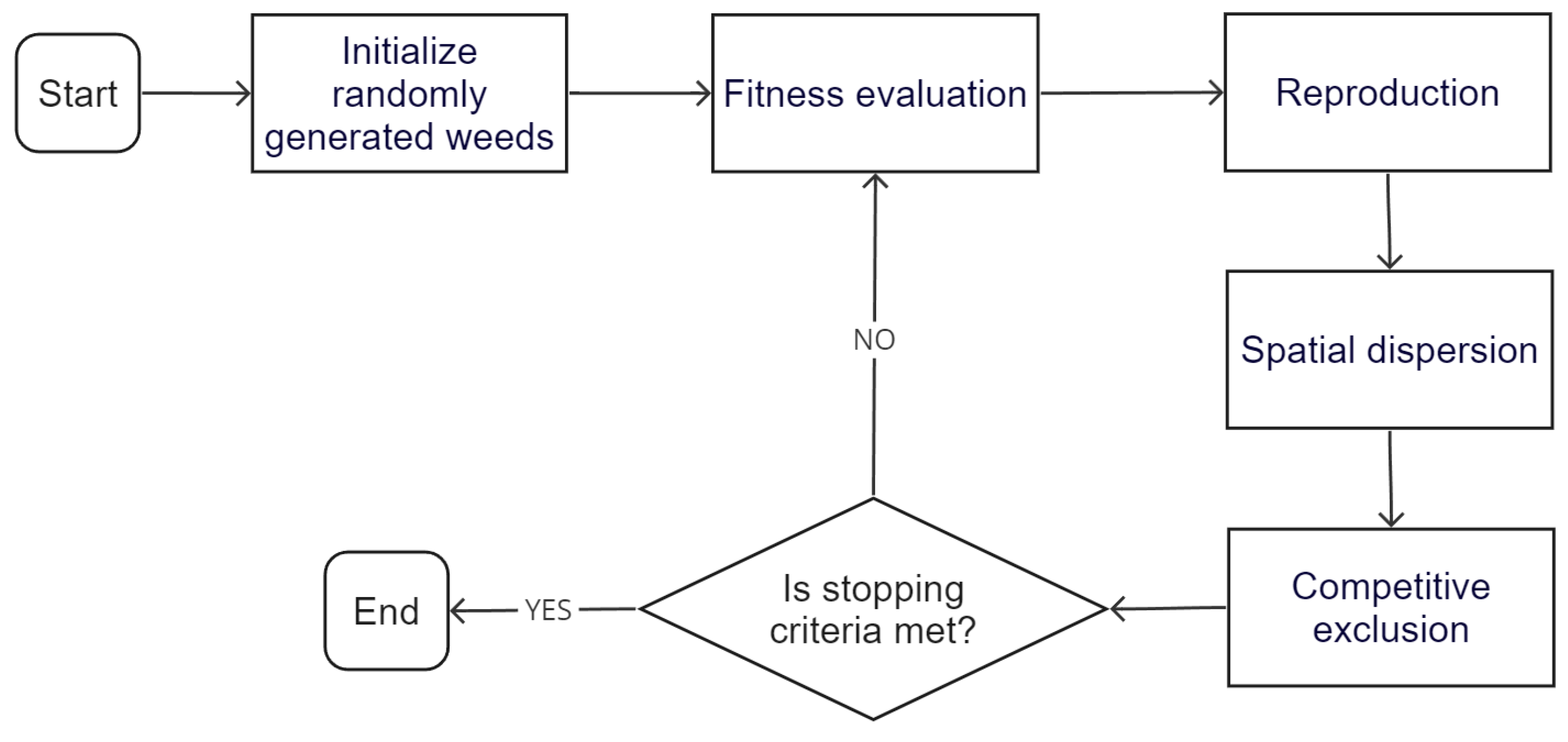
IWO draws inspiration from the growth process of invasive weeds in nature [48]. This algorithm involves a population-based approach where candidate solutions, known as weeds, compete and evolve to find optimal or near-optimal solutions to optimization problems. IWO employs mechanisms such as reproduction, competition, and migration, where weeds with better fitness values spread and dominate the search space, while less fit weeds are suppressed or eliminated. Figure 8 illustrates the implemented IWO which has the following steps:
  • Initialization: an initial population of candidate solutions, represented by weeds, is generated and randomly distributed in a d-dimensional search space.
  • Reproduction: Each candidate solution has a reproductive capacity that depends on its fitness value and the minimum and maximum fitness value of the population. The number of seeds produced by a candidate solution varies linearly from a minimum value for the solution with the worst fitness value to a maximum value for the solution with the best fitness value.
  • Spatial distribution: The generated seeds are randomly dispersed in the search space by a random function with normal distribution, with zero mean and variance decreasing over iterations. This ensures that the seeds are placed in regions far from but close to the candidate progenitor solution. The nonlinear reduction in variance favors convergence of the fittest candidate solutions and eliminates inadequate candidate solutions over time. The standard deviation of the random function is reduced at each iteration, from a predefined initial value to a final value, as calculated at each time step by Equation (19).
    σ i t e r = ( i t e r m a x i t e r ) n ( i t e r m a x ) n ( σ i n i t i a l σ f i n a l ) + σ f i n a l
    In this case, i t e r m a x is the maximum number of iterations, i t e r is the standard deviation at the current time step and n is the nonlinear modulation index which is usually set to 2.
  • Competitive exclusion: Due to the exponential growth of the population, after a few iterations, the number of candidate solutions reaches a maximum limit (Pmax). At this point, a competitive mechanism is activated to eliminate the candidate solutions with low fitness and allow the fittest candidate solutions to reproduce more. This process continues until the maximum number of iterations is reached.

3.2.4. Artificial Bee Colony

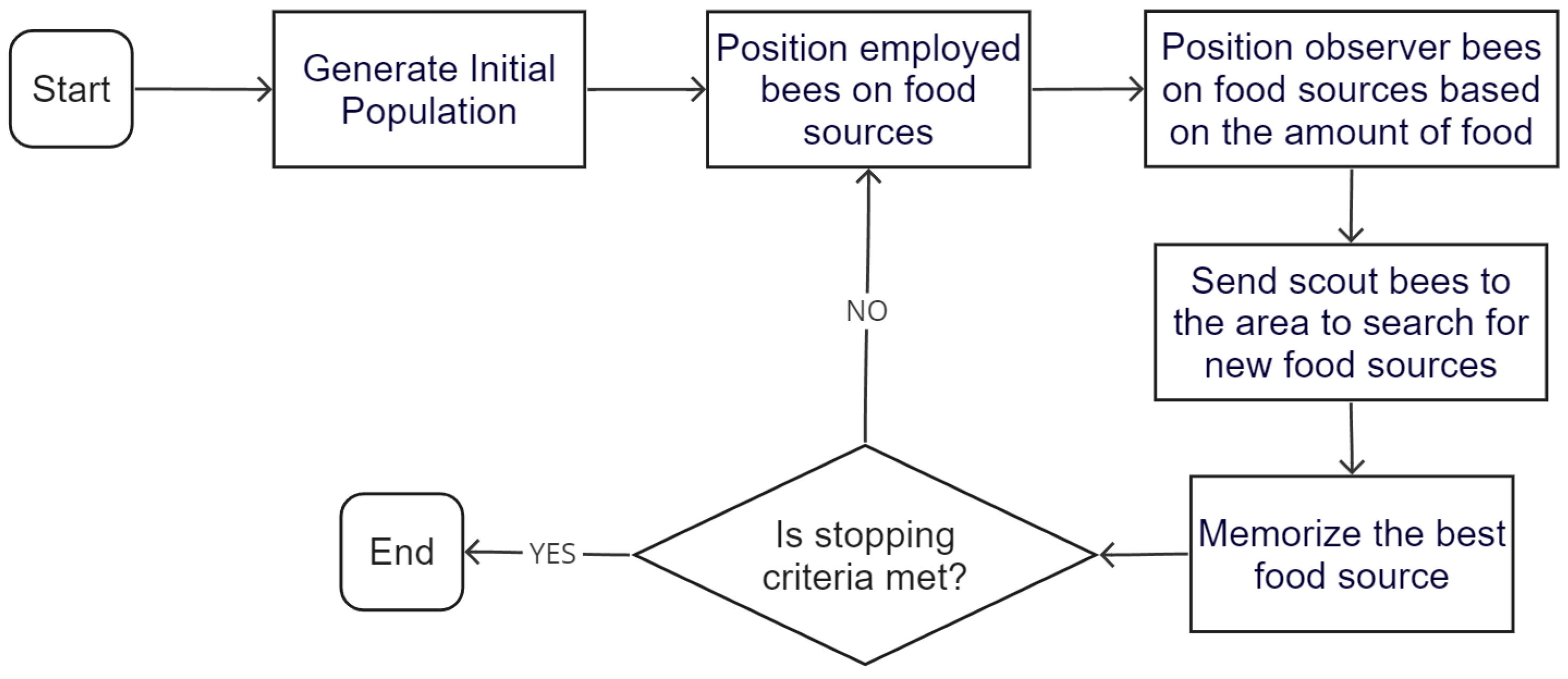
Artificial Bee Colony Optimization (ABC) is a population-based metaheuristic algorithm inspired by the behavior of honeybees [49]. ABC simulates the search for optimal solutions by employing three main groups of artificial bees: employed bees, onlookers, and scouts. Employed bees exploit known food sources (solutions) and share information about their quality with onlookers, which then choose food sources based on this information. Unpromising food sources are abandoned and replaced by scouts exploring new ones. Through iterative cycles of exploration and exploitation, ABC aims to efficiently explore the solution space, focusing on promising regions to find high-quality solutions. The flowchart of the implemented ABC approach is depicted in Figure 9. The initial phase involves the random generation of a population of solutions. Each solution is represented as a D-dimensional vector, where D is the number of optimization parameters involved in the problem. Subsequently, the population undergoes iterations through the activities of employed bees, onlookers, and scouts. The bees introduce modifications to their position (solution) based on local information, and evaluate the quality of the new source (new solution) in terms of the amount of nectar (fitness value). If the new source has a higher nectar level than the previous source, the bee retains the new position in its memory and discards the previous one. Otherwise, it retains the previous position in its memory.

4. Tests and Results

4.1. Description of the Microgrid Test Network

Figure 10 depicts the IEC test network used in this work. The data of this network is available in [50]. The protection scheme of this microgrid is described in [27]. The test network is distinguished by the presence of two circuit breakers, CB-1 and CB-2, which play a crucial role in the management and control of the network. In addition, DG was incorporated, adding flexibility to the microgrid. The aforementioned circuit breakers and the activation or deactivation of DG units define the operating scenarios that are studied. Table 2 provides a detailed breakdown of the maneuvers associated with these elements that generate 16 operational scenarios (OS).

4.2. Clustering of Operational Scenarios

The clustering of the OS presented in Table 2 is carried out with various unsupervised learning techniques to generate four clusters in each case. Four clustering techniques were evaluated, covering a total of 73 variants of these techniques. After analyzing each of these variants, it was observed that multiple approaches generated identical results. Each result was identified and numbered. Details of these clusters are given in Table 3, Table 4 and Table 5.
For example, in Table 3, it can be seen that the K-means, BIRCH and Agglomerative Hierarchical, ward, Euclidean techniques or variants yielded the following four clusters:
  • 1, 3, 13, 15.
  • 4, 8, 12, 16.
  • 5, 7, 9, 11.
  • 2, 6, 10, 14.
This set of clusters is assigned the name “Group 1”. The same procedure is repeated for each row in Table 3, Table 4 and Table 5. In all tables, the first column indicates the machine learning techniques that found the same clusters; the second column details the scenarios that belong to each of the clusters and the third column assigns a group to this set of scenarios.

4.3. Optimal Protection Coordination with Metaheuristic Techniques

Table 6 presents the results with the implemented GA. Only groups in which there were no violations of the constraints of the optimization problem are considered. Applying the GA, only 15 of the 31 proposed groups are feasible (meet all the system constraints). For each group, the first four lines indicate the operation and simulation times (in seconds) associated with each cluster, while the fifth line shows the total sum of the operation or simulation times for the group. For example, for Group 1, the first cluster given by operative scenarios 1, 3, 13 and 15 (see the first line of Table 3) presents operation and simulation times of 39.3 and 21.17, respectively. The former indicates the relays’ operation time, while the latter refers to the simulation time of the GA.
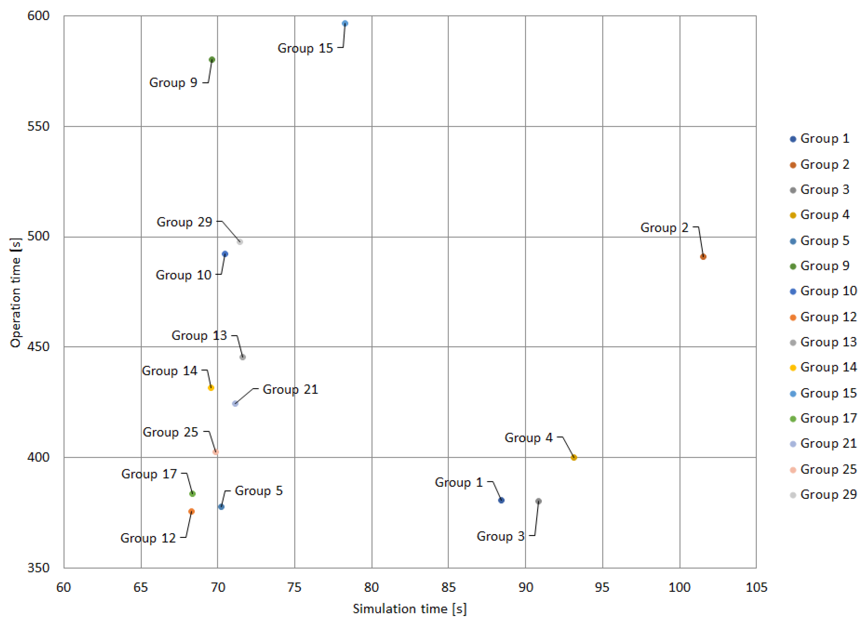
Figure 11 illustrates the results obtained by applying the GA to the protection coordination of the proposed clusters. In this case, each point in Figure 11 indicates a specific group (please refer to Table 6). The Y-axis represents the operation time, while the X-axis shows the simulation time. The solutions closest to the origin have the shortest operation and simulation times; therefore, they represent the best solutions. In this case, group 12 stands out as the best in terms of operation and simulation times. It is closely followed by groups 17, 5 and 25, which also show high-quality solutions. Note that there are some trade-offs between solutions. For example, group 9 represents a solution with a low solution time and high operation time; conversely, group 3 features a high solution time and low operation time. As the main objective function of the protection coordination problem is the minimization of the operation time, group 3 would be more desirable.
Table 7 shows the results obtained with PSO algorithm to solve the problem of protection coordination of the different groups under analysis. Note that the structure of Table 7 is similar to the structure of Table 6, where the first four lines indicate the operation and simulation times associated with each cluster, while the fifth line indicates the total operation and simulation times. In this case, only 14 of the 31 groups presented feasible solutions with the PSO approach. Figure 12 illustrates the PSO solutions described in Table 7. The solutions closest to the origin are the most desirable, since they present both low operation and simulation times. In this sense, the best-performing groups are 5, 25 and 12. Although group 1 has a reduced operation time, the simulation time is considerable.
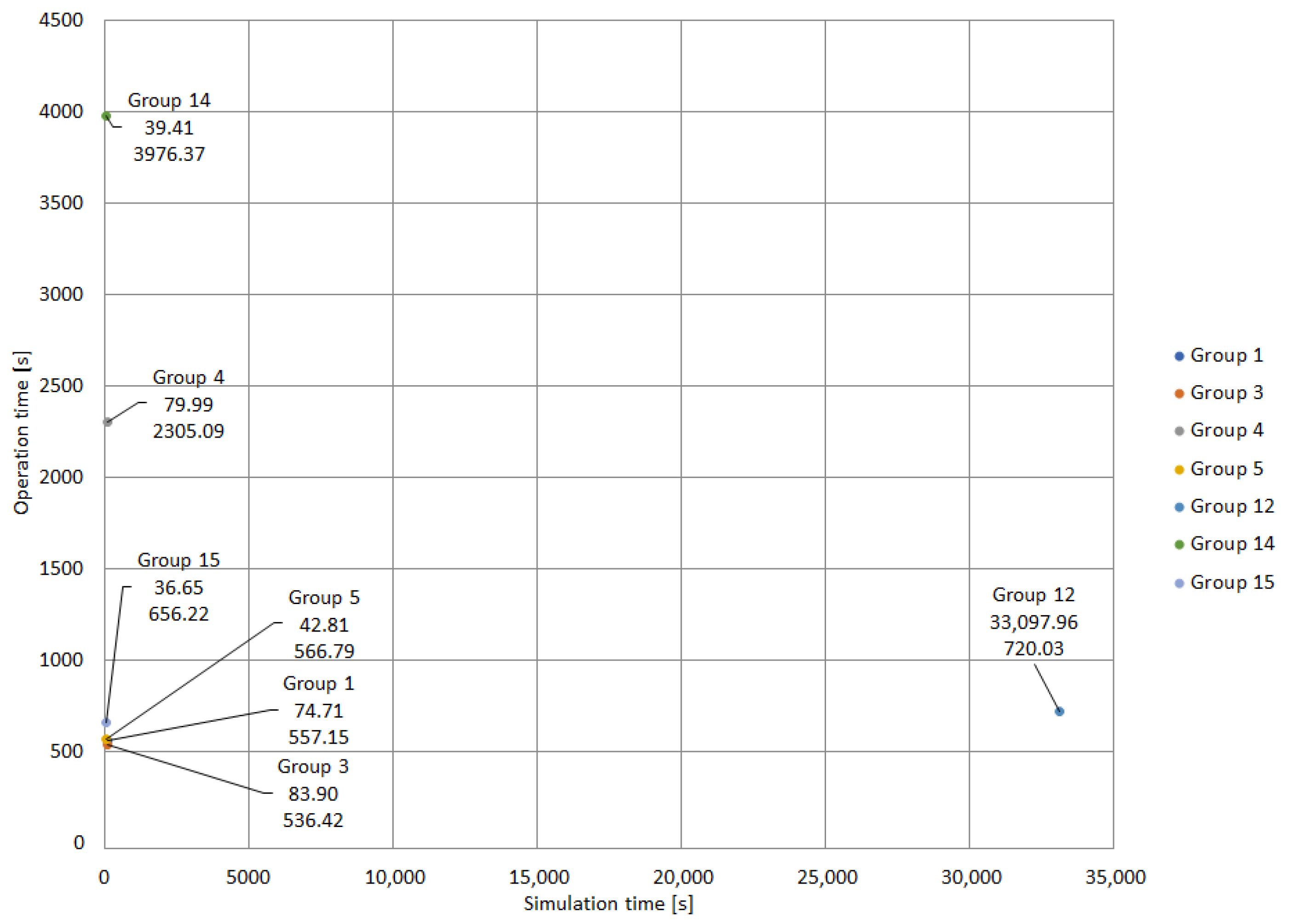
Table 8 presents the results of the protection coordination applying the IWO algorithm. It is important to highlight that, compared to other metaheuristic techniques, the IWO algorithm exhibited the lowest number of groups that achieved convergence without violations of constraints. In this case, only 7 groups of 31 obtained feasible solutions with the IWO algorithm. The structure of Table 8 is similar to the structure of Table 6. Figure 13 and Figure 14 illustrate the solutions considering both the operation and simulation times, the same way as indicated in Figure 11.
Figure 13 illustrates the groups presented in Table 8. Note that Groups 12 and 14 exhibit excessive simulation and operation times, respectively. These groups, despite presenting convergence without violations, feature an unfavorable relationship between their operation and simulation times.
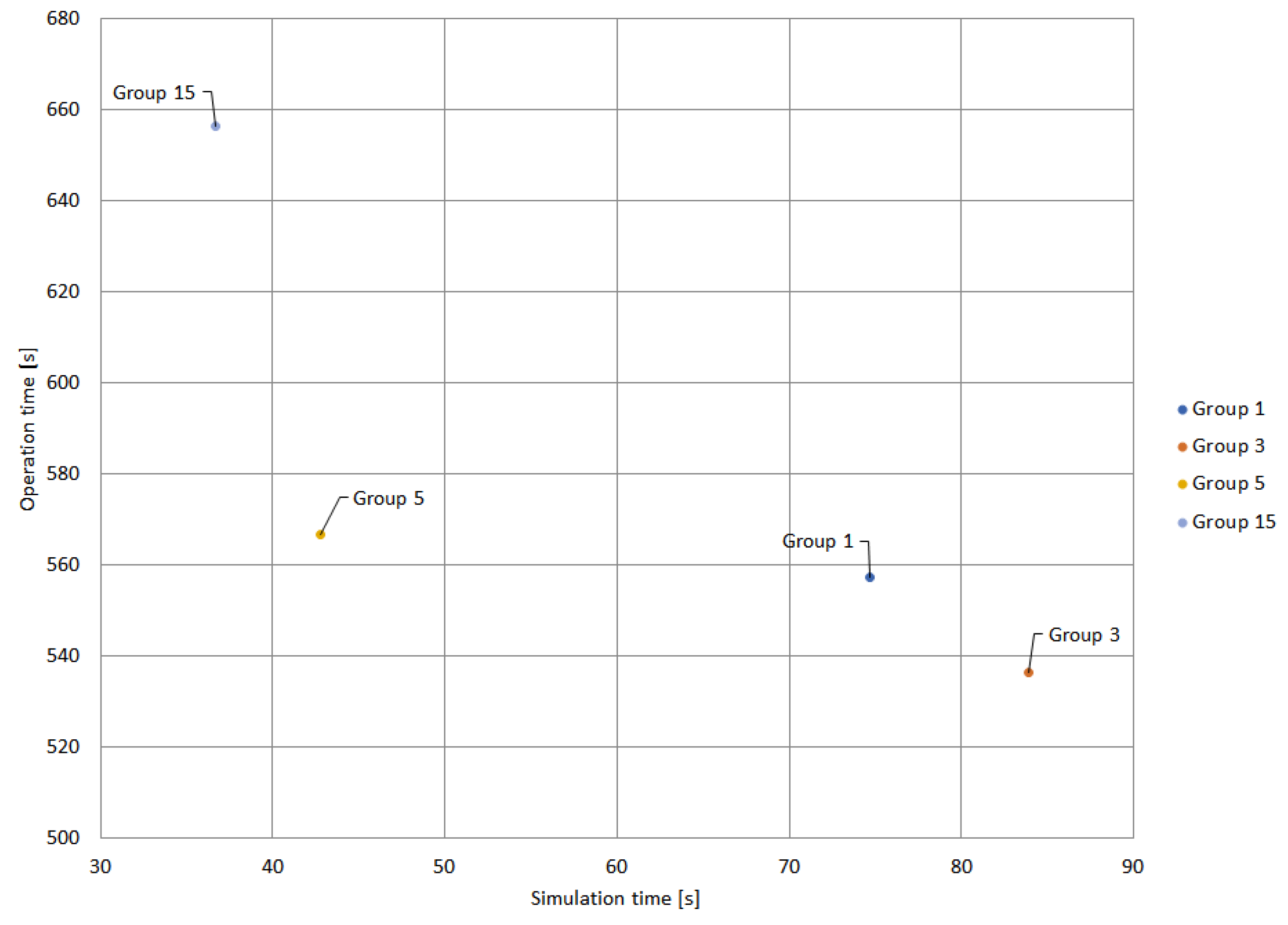
Figure 14 presents a close-up of Figure 13, where the differences in the groups that obtained the best results in terms of simulation and operation times are evident. It can be observed that although the IWO algorithm achieves convergence for a reduced number of cluster groups, the simulation times are competent. In this case, Group 5 stands out as having the best ratio between operation and simulation time. Although Group 3 stands out for its shorter operation time (536.42 s), its simulation time is considerably longer compared to Group 5. Group 15 has the best simulation time with 36.65 s, but an operation time of 656.22 which is much longer than the operation time of Group 5.
Table 9 presents the results of applying the ABC algorithm to the protection coordination problem of the text network. In this case, 15 out of the 31 Groups obtained by the clustering techniques converged without violations of constraints. The structure of Table 9 is similar to that of Table 6, indicating the operation and simulation times of each cluster within its group.
Figure 15 illustrates the groups listed in Table 9 in a similar way to Figure 11. Most of the groups exhibit operation times ranging from 300 to 800 s, while the simulation times of most groups is within the range of 70 to 80 s. Group 17 stands out as having the shortest operation and simulation time. The ABC algorithm presents competitive results, similar to those of the other metaheuristic techniques examined in this study.

4.4. Comparison of Metaheuristic Techniques

This section compares the groups of clusters that converged without violations, with the lowest operation and simulation times for each metaheuristic technique applied. The points in each graph represent specific groups that converged without violations according to the metaheuristic technique used.
In Figure 16, it is observed that group 12 (for different algorithms) presents the best performance in terms of simulation and operation time. The scale of Figure 16 was adjusted to include the response of the IWO algorithm, which has high simulation and operation times.
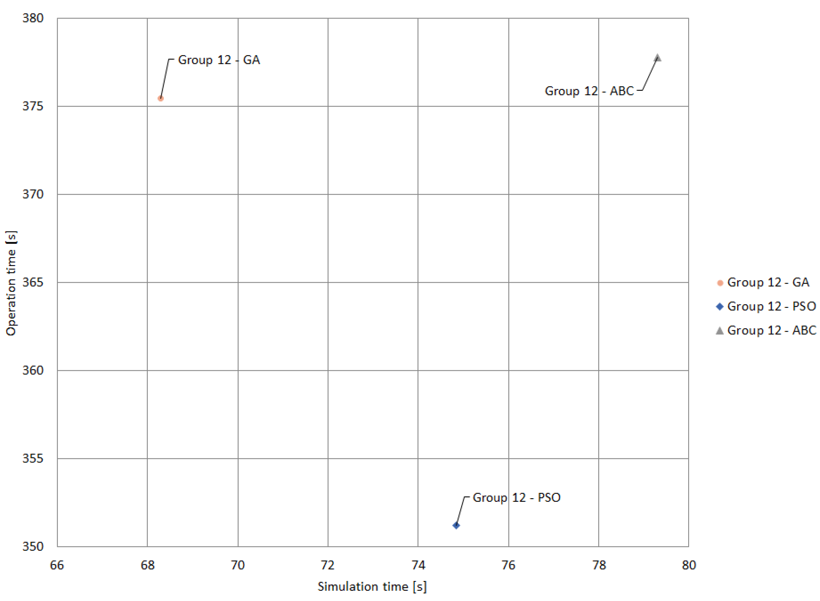
Figure 17 shows a zoom in of Figure 16, providing a more accurate visualization of the results of Group 12 with GA, PSO and ABC. It can be seen that GA has the best simulation time with 68.28 s; however, it presents the second-best operation time, with a total of 375.45 s. In contrast, the PSO Algorithm stands out with the best operation time for this group, with 351.22 s, although it has the second-best simulation time (74.83 s). On the other hand, ABC has the longest simulation and operation times.
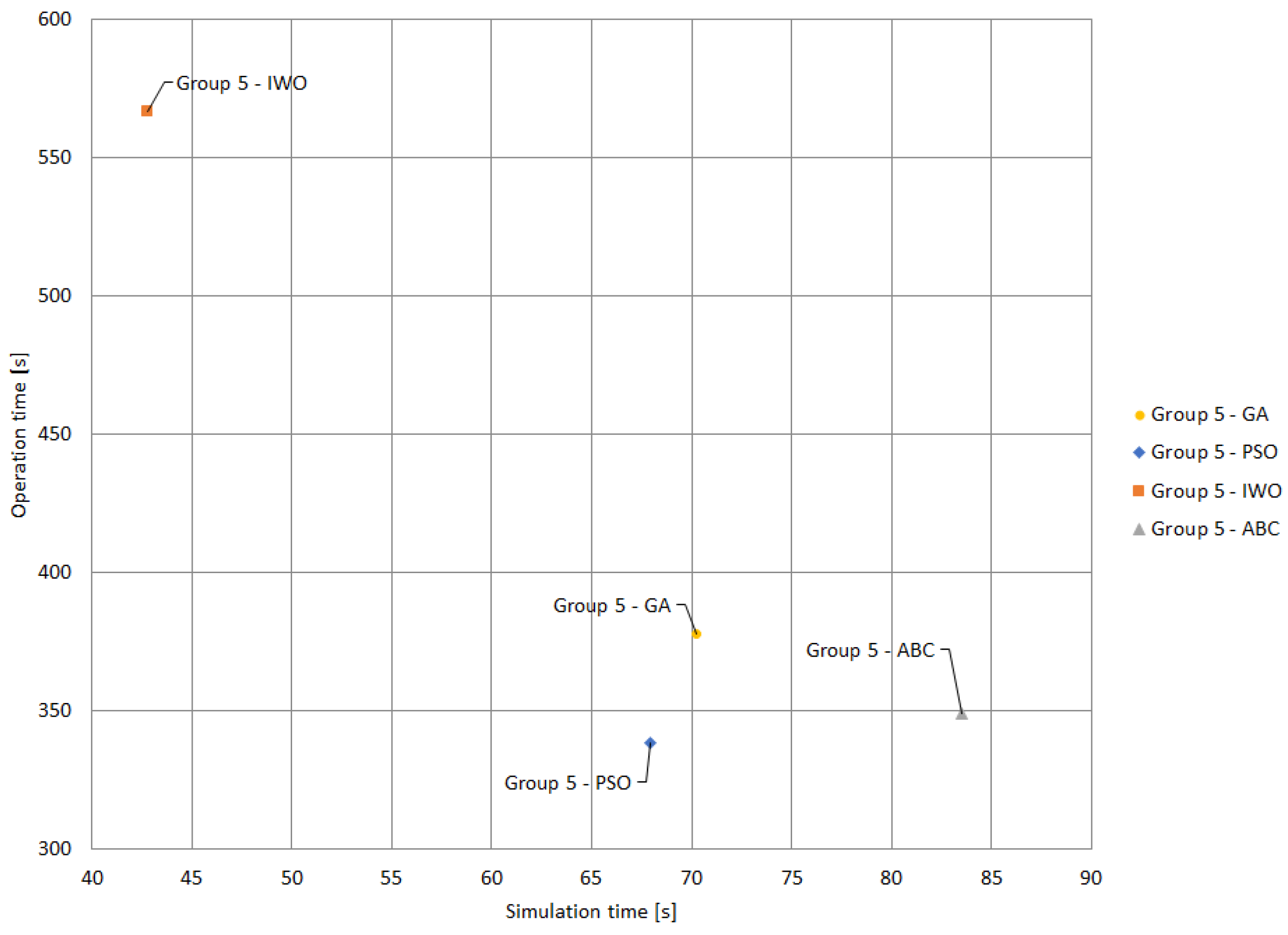
PSO and IWO obtained the best operation and simulation times with Group 5; consequently, the results of all techniques in this group were compared in Figure 18. In this case, the results obtained with PSO present the best operation time (338.37 s), along with the second-best simulation time (67.93 s). On the other hand, the IWO algorithm presents the shortest simulation time, with 42.80 s, although with the worst operation time, located at 566.78 s. The ABC algorithm stands out with the second-best operation time of 349.33 s, and the third-best simulation time, of 83.53 s. Finally, the GA algorithm recorded operation and simulation times of 377.73 and 70.20 s, respectively.
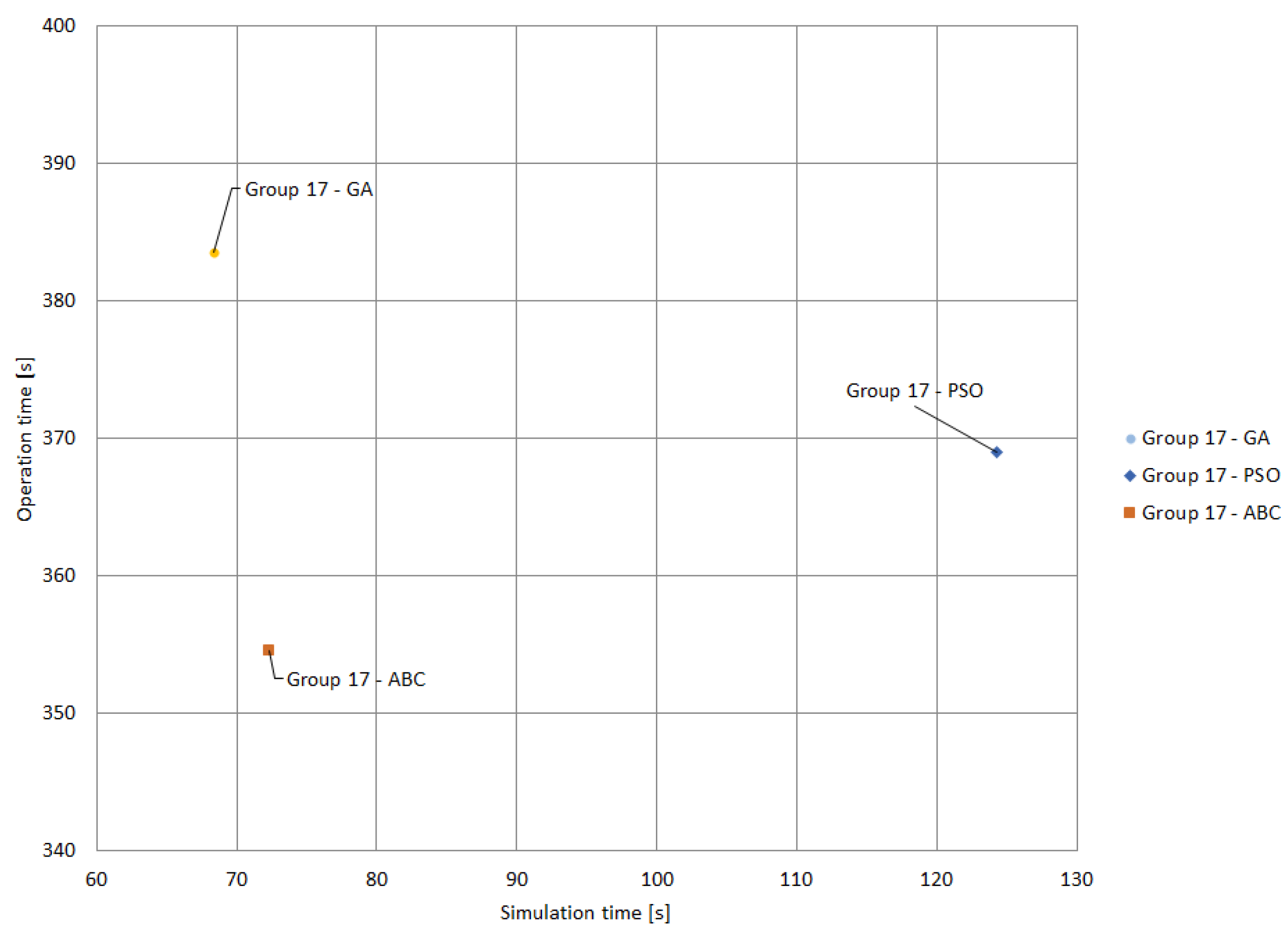
The ABC algorithm obtained the best operation and simulation times with Group 17. It should be noted that Group 17 converged without violations when using the GA and PSO algorithms, while violations were observed when applying the IWO algorithm. For this reason, the comparison is limited to three metaheuristic techniques in Figure 19. The ABC algorithm presents the shortest operation time (354.58 s), although it presents the second-best simulation time, (72.34 s). In contrast, GA has the best simulation time (68.35 s), but the worst operation time (383.52 s). Finally, PSO has the worst simulation time and the second-best operation time.
Figure 20 presents the groups of clusters exhibiting the best results for each metaheuristic technique evaluated. Cluster 12 is identified as the best for the GA algorithm, Cluster 5 for the PSO and IWO algorithms, and Cluster 17 as the best for the ABC algorithm.
In this context, Group 5 of the PSO algorithm stands out as having the best results in terms of the ratio between operation and simulation time. Although it presents the second best simulation time (67.93 s), it stands out by having the best operation time of all, totaling 338.37 s. However, IWO Group 5, despite exhibiting the best simulation time, has the worst operation time (566.78 s).
Group 17 of the ABC algorithm has the second best operation time (354.58 s) and the worst simulation time (72.34 s). Finally, Group 12 of the GA algorithm has the third best operation time, with a total of 375.45 s, and the third best simulation time, with 68.28 s.
Given the results presented, it can be concluded that Group 5 represents the most appropriate cluster configuration in terms of simulation and operation times. Furthermore, the PSO technique proved to be the most effective in the context of this study.

5. Conclusions

The results of this research allow us to conclude the viability of the integration of unsupervised machine learning techniques, metaheuristic techniques and non-standard characteristics of DOCRs in a single optimization model to solve the protection coordination problem of microgrids.
Modern microgrids may operate under different topologies, generating various operational scenarios that complicate the protection coordination problem. To tackle this issue, unsupervised machine learning techniques were used to consolidate diverse operational scenarios into distinct clusters, limited to the maximum number of configuration groups available in commercial DOCRs. On the other hand, it was found that metaheuristic techniques offer an agile resolution to the challenging nonlinear optimization problem. These solutions provide flexibility to the user by allowing a choice between results that prioritize operation time, simulation time, or the relationship between the two, thus adapting to the specific needs of the user.
The performance of each metaheuristic technique was compared, examining the trade-offs between operation time and simulation time graphically. The best group for GA was Group 12; for PSO and IWO, it was group 5; and for ABC, it was group 17. The optimal performance was observed in Group 5 obtained by PSO which was generated from variants of the hierarchical agglomerative clustering algorithm.

Author Contributions

Conceptualization, J.E.S.-R., S.D.S.-Z., J.M.L.-L., N.M.-G. and W.M.V.-A.; Formal analysis, J.E.S.-R., S.D.S.-Z., J.M.L.-L., N.M.-G. and W.M.V.-A.; Funding acquisition, J.M.L.-L., N.M.-G. and W.M.V.-A.; Investigation, N.M.-G., S.D.S.-Z. and J.M.L.-L.; Methodology, J.E.S.-R., S.D.S.-Z., J.M.L.-L., N.M.-G. and W.M.V.-A.; Project administration, S.D.S.-Z., J.M.L.-L., N.M.-G. and W.M.V.-A.; Resources, J.E.S.-R., S.D.S.-Z., J.M.L.-L. and N.M.-G.; Software, J.E.S.-R. and S.D.S.-Z.; Supervision, J.M.L.-L., N.M.-G. and W.M.V.-A.; Validation, J.E.S.-R., S.D.S.-Z., J.M.L.-L., N.M.-G. and W.M.V.-A.; Visualization, J.E.S.-R., S.D.S.-Z., J.M.L.-L., N.M.-G. and W.M.V.-A.; Writing—original draft, J.E.S.-R. and S.D.S.-Z.; Writing—review and editing, J.E.S.-R., S.D.S.-Z., J.M.L.-L., N.M.-G. and W.M.V.-A. All authors have read and agreed to the published version of the manuscript.

Funding

This research was funded by Universidad de Antioquia (Medellin, 050010, Colombia) and Institución Universitaria Pascual Bravo (Medellin, 050036, Colombia).

Data Availability Statement

Data are contained within the article.

Acknowledgments

The authors gratefully acknowledge the financial support provided by the Colombian Ministry of Science, Technology, and Innovation “MinCiencias” through “Patrimonio Autónomo Fondo Nacional de Financiamiento para la Ciencia, la Tecnología y la Innovación, Francisco José de Caldas” (Perseo alliance Contract No. 112721-392-2023).

Conflicts of Interest

The authors declare no conflicts of interest.

Appendix A. Distances Used in Hierarchical Clustering

  • The Minkowski distance is a generalized distance measure that can be adjusted by the variable p to calculate the distance between two data points in different ways. Because of this, it is also known as Lp-norm distance and is calculated as given in Equation (A1). The Manhattan, Euclidean and Chebychev distances result, respectively, from adjusting p = 1 , p = 2 , and p = in Equation (A1).
    M i n k o w s k i d i s t a n c e = ( i = 1 n x i y i p ) 1 p
  • The standardized Euclidean distance between two n-dimensional vectors u and v is given in Equation (A2), where V [ x i ] is the variance computed over all the i’th components of the points.
    S e u c l i d e a n d i s t a n c e = ( u i v i ) 2 V x i
  • The squared Euclidean distance between vectors u and v, is indicated in Equation (A3).
    S q e u c l i d e a n d i s t a n c e = u v 2 2
  • The cosine distance between vectors u and v, is indicated in Equation (A4), where 2 is the 2-norm of its argument ∗, and u · v is the dot product of u and v, where v ¯ is the mean of the elements of vector v, and x · y is the dot product of x and y.
    C o s i n e d i s t a n c e = 1 u · v u 2 v 2
  • The correlation distance between vectors u and v is indicated in Equation (A5).
    C o r r e l a t i o n d i s t a n c e = 1 ( u u ¯ ) · ( v v ¯ ) ( u u ¯ ) 2 ( v v ¯ ) 2
  • The Hamming distance between 1-D arrays u and v, is the proportion of disagreeing components in u and v. If u and v are boolean vectors, the Hamming distance is given by Equation (A6), where c x j is the number of occurrences of u [ k ] = i and v [ k ] = j for k < n .
    H a m m i n g d i s t a n c e = c 01 + c 10 n
  • The Jaccard–Needham dissimilarity between two boolean 1-D arrays is computed as indicated in Equation (A7), where c x j is the number of occurrences of u [ k ] = i and v [ k ] = j for k < n .
    J a c c a r d d i s t a n c e = c T F + c F T c T T + c F T + c T F
  • The Kulczynski dissimilarity between two boolean 1-D arrays is computed as indicated in Equation (A8), where c x j is the number of occurrences of u [ k ] = i and v [ k ] = j for k 0 , 1 , , n 1 .
    K u l c z y n s k i d i s t a n c e = c 11 c 01 + c 10
  • The Chebyshev distance between two 1-D arrays u and v is defined in Equation (A9).
    C h e b y s h e v d i s t a n c e = m a x i u i v i
  • The Canberra distance between two 1-D arrays, u and v is given by Equation (A10).
    C a n b e r r a d i s t a n c e = i u i v i u i + v i
  • The Bray–Curtis distance between two 1-D arrays is given by Equation (A11). The Bray–Curtis distance is in the range [ 0 , 1 ] if all coordinates are positive, and is undefined if the inputs are of length zero.
    B r a y C u r t i s d i s t a n c e = u i v i u i + v i
  • The Mahalanobis distance between 1-D arrays u and v is defined as indicated in Equation (A12), where V is the covariance matrix.
    M a h a l a n o b i s d i s t a n c e = ( u v ) V 1 ( u v ) T )
  • The Yule dissimilarity between two boolean 1-D arrays is given by Equation (A13), where c x j is the number of occurrences of u [ k ] = i and v [ k ] = j for k < n and R = 2.0 c T F c F T .
    Y u l e d i s t a n c e = R c T T c F F + R 2
  • The Dice dissimilarity between two boolean 1-D arrays is given by Equation (A14), where c x j is the number of occurrences of u [ k ] = i and v [ k ] = j for k < n .
    D i c e d i s t a n c e = c T F + c F T 2 c T T + c F T + c T F
  • The Rogers–Tanimoto dissimilarity between two boolean 1-D arrays u and v, is defined in Equation (A15), where c x j is the number of occurrences of u [ k ] = i and v [ k ] = j for k < n and R = 2 ( c T F + c F T ) .
    R o g e r s T a n i m o t o d i s t a n c e = R c T T + c F F + R
  • The Russell–Rao dissimilarity between two boolean 1-D arrays u and v, is defined in Equation (A16), where c x j is the number of occurrences of u [ k ] = i and v [ k ] = j for k < n .
    R u s s e l l R a o d i s t a n c e = n c T T n
  • The Sokal–Michener dissimilarity between two boolean 1-D arrays u and v, is defined in Equation (A17), where c x j is the number of occurrences of u [ k ] = i and v [ k ] = j for k < n , R = 2 ( c T F + c F T ) and S = c F F + c T T .
    S o k a l M i c h e n e r d i s t a n c e = R S + R
  • The Sokal–Sneath dissimilarity between two boolean 1-D arrays u and v is given by Equation (A18), where c x j is the number of occurrences of u [ k ] = i and v [ k ] = j for k < n and R = 2 ( c T F + c F T ) .
    S o k a l S n e a t h d i s t a n c e = R c T T + R

References

  1. Saldarriaga-Zuluaga, S.D.; Lopez-Lezama, J.M.; Muñoz-Galeano, N. Protection coordination in microgrids: Current weaknesses, available solutions and future challenges. IEEE Lat. Am. Trans. 2020, 18, 1715–1723. [Google Scholar] [CrossRef]
  2. Peyghami, S.; Fotuhi-Firuzabad, M.; Blaabjerg, F. Reliability Evaluation in Microgrids with Non-Exponential Failure Rates of Power Units. IEEE Syst. J. 2020, 14, 2861–2872. [Google Scholar] [CrossRef]
  3. Zhong, W.; Wang, L.; Liu, Z.; Hou, S. Reliability Evaluation and Improvement of Islanded Microgrid Considering Operation Failures of Power Electronic Equipment. J. Mod. Power Syst. Clean Energy 2020, 8, 111–123. [Google Scholar] [CrossRef]
  4. Muhtadi, A.; Pandit, D.; Nguyen, N.; Mitra, J. Distributed Energy Resources Based Microgrid: Review of Architecture, Control, and Reliability. IEEE Trans. Ind. Appl. 2021, 57, 2223–2235. [Google Scholar] [CrossRef]
  5. Muzi, F.; Calcara, L.; Pompili, M.; Fioravanti, A. A microgrid control strategy to save energy and curb global carbon emissions. In Proceedings of the 2019 IEEE International Conference on Environment and Electrical Engineering and 2019 IEEE Industrial and Commercial Power Systems Europe (EEEIC/I&CPS Europe), Genova, Italy, 11–14 June 2019; pp. 1–4. [Google Scholar] [CrossRef]
  6. Fang, S.; Khan, I.; Liao, R. Stochastic Robust Hybrid Energy Storage System Sizing for Shipboard Microgrid Decarbonization. In Proceedings of the 2022 IEEE/IAS Industrial and Commercial Power System Asia (I&CPS Asia), Shanghai, China, 8–11 July 2022; pp. 706–711. [Google Scholar] [CrossRef]
  7. Balcu, I.; Ciucanu, I.; Macarie, C.; Taranu, B.; Ciupageanu, D.A.; Lazaroiu, G.; Dumbrava, V. Decarbonization of Low Power Applications through Methanation Facilities Integration. In Proceedings of the 2019 IEEE PES Innovative Smart Grid Technologies Europe (ISGT-Europe), Bucharest, Romania, 29 September–2 October 2019; pp. 1–5. [Google Scholar] [CrossRef]
  8. Villada-Duque, F.; Lopez-Lezama, J.M.; Muñoz-Galeano, N. Effects of incentives for renewable energy in Colombia. Ing. Y Univ. 2017, 21, 257–272. [Google Scholar] [CrossRef]
  9. Glória, L.L.; Righetto, S.B.; de Oliveira, D.B.S.; Martins, M.A.I.; Kraemer, R.A.S.; Ludwig, M.A. Microgrids and Virtual Power Plants: Integration Possibilities. In Proceedings of the 2022 2nd Asian Conference on Innovation in Technology (ASIANCON), Ravet, India, 26–28 August 2022; pp. 1–4. [Google Scholar] [CrossRef]
  10. Bani-Ahmed, A.; Rashidi, M.; Nasiri, A.; Hosseini, H. Reliability Analysis of a Decentralized Microgrid Control Architecture. IEEE Trans. Smart Grid 2019, 10, 3910–3918. [Google Scholar] [CrossRef]
  11. Bonetti, C.; Bianchotti, J.; Vega, J.; Puccini, G. Optimal Segmentation of Electrical Distribution Networks. IEEE Lat. Am. Trans. 2021, 19, 1375–1382. [Google Scholar] [CrossRef]
  12. Paudel, A.; Chaudhari, K.; Long, C.; Gooi, H.B. Peer-to-Peer Energy Trading in a Prosumer-Based Community Microgrid: A Game-Theoretic Model. IEEE Trans. Ind. Electron. 2019, 66, 6087–6097. [Google Scholar] [CrossRef]
  13. Che, L.; Zhang, X.; Shahidehpour, M.; Alabdulwahab, A.; Abusorrah, A. Optimal Interconnection Planning of Community Microgrids with Renewable Energy Sources. IEEE Trans. Smart Grid 2017, 8, 1054–1063. [Google Scholar] [CrossRef]
  14. Zeineldin, H.H.; Mohamed, Y.A.R.I.; Khadkikar, V.; Pandi, V.R. A Protection Coordination Index for Evaluating Distributed Generation Impacts on Protection for Meshed Distribution Systems. IEEE Trans. Smart Grid 2013, 4, 1523–1532. [Google Scholar] [CrossRef]
  15. Ehrenberger, J.; Švec, J. Directional Overcurrent Relays Coordination Problems in Distributed Generation Systems. Energies 2017, 10, 1452. [Google Scholar] [CrossRef]
  16. Noghabi, A.S.; Mashhadi, H.R.; Sadeh, J. Optimal Coordination of Directional Overcurrent Relays Considering Different Network Topologies Using Interval Linear Programming. IEEE Trans. Power Deliv. 2010, 25, 1348–1354. [Google Scholar] [CrossRef]
  17. So, C.; Li, K. Time coordination method for power system protection by evolutionary algorithm. IEEE Trans. Ind. Appl. 2000, 36, 1235–1240. [Google Scholar] [CrossRef]
  18. Razavi, F.; Abyaneh, H.A.; Al-Dabbagh, M.; Mohammadi, R.; Torkaman, H. A new comprehensive genetic algorithm method for optimal overcurrent relays coordination. Electr. Power Syst. Res. 2008, 78, 713–720. [Google Scholar] [CrossRef]
  19. Kiliçkiran, H.C.; Şengör, İ.; Akdemir, H.; Kekezoğlu, B.; Erdinç, O.; Paterakis, N.G. Power system protection with digital overcurrent relays: A review of non-standard characteristics. Electr. Power Syst. Res. 2018, 164, 89–102. [Google Scholar] [CrossRef]
  20. Alasali, F.; Zarour, E.; Holderbaum, W.; Nusair, K.N. Highly Fast Innovative Overcurrent Protection Scheme for Microgrid Using Metaheuristic Optimization Algorithms and Nonstandard Tripping Characteristics. IEEE Access 2022, 10, 42208–42231. [Google Scholar] [CrossRef]
  21. Saldarriaga-Zuluaga, S.D.; López-Lezama, J.M.; Muñoz-Galeano, N. Adaptive protection coordination scheme in microgrids using directional over-current relays with non-standard characteristics. Heliyon 2021, 7, e06665. [Google Scholar] [CrossRef] [PubMed]
  22. So, C.; Li, K. Intelligent method for protection coordination. In Proceedings of the 2004 IEEE International Conference on Electric Utility Deregulation, Restructuring and Power Technologies, Hong Kong, China, 5–8 April 2004; Volume 1, pp. 378–382. [Google Scholar] [CrossRef]
  23. Mohammadi, R.; Abyaneh, H.; Razavi, F.; Al-Dabbagh, M.; Sadeghi, S. Optimal relays coordination efficient method in interconnected power systems. J. Electr. Eng. 2010, 61, 75. [Google Scholar] [CrossRef]
  24. Baghaee, H.R.; Mirsalim, M.; Gharehpetian, G.B.; Talebi, H.A. MOPSO/FDMT-based Pareto-optimal solution for coordination of overcurrent relays in interconnected networks and multi-DER microgrids. IET Gener. Transm. Distrib. 2018, 12, 2871–2886. [Google Scholar] [CrossRef]
  25. Saldarriaga-Zuluaga, S.D.; López-Lezama, J.M.; Muñoz-Galeano, N. Optimal coordination of overcurrent relays in microgrids considering a non-standard characteristic. Energies 2020, 13, 922. [Google Scholar] [CrossRef]
  26. Saldarriaga-Zuluaga, S.D.; Lopez-Lezama, J.M.; Munoz-Galeano, N. Optimal coordination of over-current relays in microgrids considering multiple characteristic curves. Alex. Eng. J. 2021, 60, 2093–2113. [Google Scholar] [CrossRef]
  27. Saad, S.M.; El-Naily, N.; Mohamed, F.A. A new constraint considering maximum PSM of industrial over-current relays to enhance the performance of the optimization techniques for microgrid protection schemes. Sustain. Cities Soc. 2019, 44, 445–457. [Google Scholar] [CrossRef]
  28. Ojaghi, M.; Mohammadi, V. Use of Clustering to Reduce the Number of Different Setting Groups for Adaptive Coordination of Overcurrent Relays. IEEE Trans. Power Deliv. 2018, 33, 1204–1212. [Google Scholar] [CrossRef]
  29. Ghadiri, S.M.E.; Mazlumi, K. Adaptive protection scheme for microgrids based on SOM clustering technique. Appl. Soft Comput. 2020, 88, 106062. [Google Scholar] [CrossRef]
  30. Saldarriaga-Zuluaga, S.D.; López-Lezama, J.M.; Muñoz-Galeano, N. Optimal coordination of over-current relays in microgrids using unsupervised learning techniques. Appl. Sci. 2021, 11, 1241. [Google Scholar] [CrossRef]
  31. Chabanloo, R.M.; Safari, M.; Roshanagh, R.G. Reducing the scenarios of network topology changes for adaptive coordination of overcurrent relays using hybrid GA–LP. IET Gener. Transm. Distrib. 2018, 12, 5879–5890. [Google Scholar] [CrossRef]
  32. IEC 60255-3; Electrical Relays-Part 3: Single Input Energizing Quantity Measuring Relays with Dependent or Independent Time. IEC: Geneve, Switzerland, 1989.
  33. IEEE C37.112-1996; IEEE Standard Inverse-Time Characteristic Equations for Overcurrent Relays. IEEE SA: Piscataway, NJ, USA, 1997.
  34. Bedekar, P.P.; Bhide, S.R.; Kale, V.S. Optimum coordination of overcurrent relay timing using simplex method. Electr. Power Components Syst. 2010, 38, 1175–1193. [Google Scholar] [CrossRef]
  35. Bedekar, P.P.; Bhide, S.R.; Kale, V.S. Coordination of overcurrent relays in distribution system using linear programming technique. In Proceedings of the 2009 International Conference on Control, Automation, Communication and Energy Conservation, Perundurai, India, 4–6 June 2009; pp. 1–4. [Google Scholar]
  36. Saravanan, R.; Sujatha, P. A State of Art Techniques on Machine Learning Algorithms: A Perspective of Supervised Learning Approaches in Data Classification. In Proceedings of the 2018 Second International Conference on Intelligent Computing and Control Systems (ICICCS), Madurai, India, 14–15 June 2018; pp. 945–949. [Google Scholar] [CrossRef]
  37. Pascual, D.; Pla, F.; Sánchez, S. Algoritmos de agrupamiento. In Método Informáticos Avanzados; Publicacions de la Universitat Jaume I: Castelló, Spain, 2007; pp. 164–174. [Google Scholar]
  38. Franco-Árcega, A.; Sobrevilla-Sólis, V.I.; de Jesús Gutiérrez-Sánchez, M.; García-Islas, L.H.; Suárez-Navarrete, A.; Rueda-Soriano, E. Sistema de enseñanza para la técnica de agrupamiento k-means. Pädi Boletín Científico Cienc. Básicas E Ing. ICBI 2021, 9, 53–58. [Google Scholar] [CrossRef]
  39. Feizollah, A.; Anuar, N.B.; Salleh, R.; Amalina, F. Comparative study of k-means and mini batch k-means clustering algorithms in android malware detection using network traffic analysis. In Proceedings of the 2014 International Symposium on Biometrics and Security Technologies (ISBAST), Kuala Lumpur, Malaysia, 26–27 August 2014; pp. 193–197. [Google Scholar] [CrossRef]
  40. K-Means vs. Mini Batch K-Means: A Comparison. Available online: https://upcommons.upc.edu/bitstream/handle/2117/23414/R13-8.pdf (accessed on 16 November 2023).
  41. Murugesan, K.; Zhang, J. Algoritmo de agrupamiento de medias K de bisección híbrida. In Proceedings of the Conferencia Internacional 2011 Sobre informáTica Empresarial e Informatización Global, Shanghai, China, 29–31 July 2011. [Google Scholar] [CrossRef]
  42. Du, H.; Li, Y. An Improved BIRCH Clustering Algorithm and Application in Thermal Power. In Proceedings of the 2010 International Conference on Web Information Systems and Mining, Sanya, China, 23–24 October 2010; Volume 1, pp. 53–56. [Google Scholar] [CrossRef]
  43. McLachlan, G.J.; Rathnayake, S. On the number of components in a Gaussian mixture model. Wiley Interdiscip. Rev. Data Min. Knowl. Discov. 2014, 4, 341–355. [Google Scholar] [CrossRef]
  44. Patel, E.; Singh Kushwaha, D. Clustering Cloud Workloads: K-Means vs Gaussian Mixture Model. Procedia Comput. Sci. 2020, 171, 158–167. [Google Scholar] [CrossRef]
  45. Pedregosa, F.; Varoquaux, G.; Gramfort, A.; Michel, V.; Thirion, B.; Grisel, O.; Blondel, M.; Prettenhofer, P.; Weiss, R.; Dubourg, V.; et al. Sklearn. Cluster. AgglomerativeClustering—Scikit-Learn 0.24. 2 Documentation. 2021. Available online: https://scikit-learn.org/stable/modules/generated/sklearn.cluster.AgglomerativeClustering.html (accessed on 30 January 2023).
  46. Gu, X.; Angelov, P.P.; Kangin, D.; Principe, J.C. A new type of distance metric and its use for clustering. Evol. Syst. 2017, 8, 167–177. [Google Scholar] [CrossRef]
  47. SciPy, d. Scipy.spatial.distance.pdist—SciPy v1.11.3 Manual. 2021. Available online: https://docs.scipy.org/doc/scipy/reference/generated/scipy.spatial.distance.pdist.html (accessed on 30 January 2023).
  48. Xing, B.; Gao, W.J. Invasive Weed Optimization Algorithm. In Innovative Computational Intelligence: A Rough Guide to 134 Clever Algorithms; Springer International Publishing: Cham, Switzerland, 2014; pp. 177–181. [Google Scholar] [CrossRef]
  49. Karaboga, D.; Akay, B. A comparative study of Artificial Bee Colony algorithm. Appl. Math. Comput. 2009, 214, 108–132. [Google Scholar] [CrossRef]
  50. Kar, S.; Samantaray, S.R.; Zadeh, M.D. Data-Mining Model Based Intelligent Differential Microgrid Protection Scheme. IEEE Syst. J. 2017, 11, 1161–1169. [Google Scholar] [CrossRef]
Figure 1. Representation of candidates for a solution of a 4-relay system.
Energies 17 00210 g001
Figure 2. Flowchart of the implemented methodology.
Energies 17 00210 g002
Figure 3. Flowchart of K-Means clustering algorithm.
Energies 17 00210 g003
Figure 4. Flowchart of the BIRCH algorithm.
Energies 17 00210 g004
Figure 5. Flowchart of a GMM.
Energies 17 00210 g005
Figure 6. Flowchart of the implemented GA.
Energies 17 00210 g006
Figure 7. Flowchart of the implemented PSO.
Energies 17 00210 g007
Figure 8. Flowchart of the implemented IWO.
Energies 17 00210 g008
Figure 9. Flowchart of the implemented ABC.
Energies 17 00210 g009
Figure 10. Benchmark IEC microgrid.
Energies 17 00210 g010
Figure 11. Best performing groups with GA.
Energies 17 00210 g011
Figure 12. Best performing groups with PSO.
Energies 17 00210 g012
Figure 13. Best performing groups with IWO.
Energies 17 00210 g013
Figure 14. Best performing groups with IWO (zoom in).
Energies 17 00210 g014
Figure 15. Best performing groups with ABC.
Energies 17 00210 g015
Figure 16. Performance of Group 12 for different algorithms.
Energies 17 00210 g016
Figure 17. Performance of Group 12 for different algorithms (zoom in).
Energies 17 00210 g017
Figure 18. Comparison of results for Group 5 with different metaheuristics.
Energies 17 00210 g018
Figure 19. Comparison of results for Group 17 with different metaheuristics.
Energies 17 00210 g019
Figure 20. Comparison of the best result of each metaheuristic technique.
Energies 17 00210 g020
Table 1. Knowledge gap.
PaperUnsupervised Machine
Learning Techniques
Metaheuristic
Techniques
Non-Standard
Characteristics
[17,18,22,23,24,31] X
[20,21,25,26,27] XX
[28]X
[29,30]XX
ProposedXXX
Table 2. Microgrid operational scenarios (OS).
OSGridCB-1CB-2DG1DG2DG3DG4
OS1onopenopenoffoffoffoff
OS2onopenopenonononon
OS3onopenopenononoffoff
OS4offopenopenonononon
OS5onclosedclosedoffoffoffoff
OS6onclosedclosedonononon
OS7onclosedclosedononoffoff
OS8offclosedcloseonononon
OS9onclosedopenoffoffoffoff
OS10onclosedopenonononon
OS11onclosedopenononoffoff
OS12offcloseopenonononon
OS13onopenclosedoffoffoffoff
OS14onopenclosedonononon
OS15onopenclosedononoffoff
OS16offopenclosedonononon
Table 3. Results of clustering analysis (1).
Unsupervised Machine Learning TechniquesClustersGroupings
K-Means
BIRCH
Agglomerative Hierarchical, ward, Euclidean
1, 3, 13, 15Group 1
4, 8, 12, 16
5, 7, 9, 11
2, 6, 10, 14
Mini Batch K-Means4, 8, 12, 16Group 2
1, 2, 3, 5, 13, 14, 15
7, 9, 10, 11
6
Bisecting K-Means4, 8, 12, 16Group 3
5, 14
6, 7, 9, 10, 11
1, 2, 3, 13, 15
Gaussian Mixture Model4, 8, 12, 16Group 4
1, 2, 3, 13, 15
5, 6, 7, 14
9, 10, 11
Agglomerative Hierarchical, complete, Euclidean
Agglomerative Hierarchical, complete, sqeuclidean
Agglomerative Hierarchical, complete, cityblock
Agglomerative Hierarchical, complete, minkowski
Agglomerative Hierarchical, complete, l2
Agglomerative Hierarchical, complete, manhattan
Agglomerative Hierarchical, complete, l1
Agglomerative Hierarchical, average, cityblock
Agglomerative Hierarchical, average, manhattan
Agglomerative Hierarchical, average, l1
1, 2, 3, 13, 14, 15Group 5
5, 7, 9, 11
6, 10
4, 8, 12, 16
Agglomerative Hierarchical, complete, cosine1, 2, 3, 5, 7, 9, 11, 13, 14, 15Group 6
8, 12, 16
4
6, 10
Agglomerative Hierarchical, complete, hamming
Agglomerative Hierarchical, complete, matching
2, 3, 4, 10, 11, 12, 14, 15, 16Group 7
1, 5, 7, 9, 13
6
8
Agglomerative Hierarchical, complete, jaccard2, 3, 4, 5, 6, 7, 8, 9, 10, 11, 12Group 8
1, 13
14, 15
16
Agglomerative Hierarchical, complete, rogerstanimoto
Agglomerative Hierarchical, complete, dice
Agglomerative Hierarchical, complete, sokalmichener
Agglomerative Hierarchical, complete, sokalsneath
Agglomerative Hierarchical, average, rogerstanimoto
Agglomerative Hierarchical, average, dice
Agglomerative Hierarchical, average, sokalmichener
5, 7, 9, 11Group 9
1, 13
2, 3, 4, 15
6, 8, 10, 12, 14, 16
Agglomerative Hierarchical, complete, chebyshev2, 5, 7, 9, 10, 11, 14Group 10
1, 3, 13, 15
6
4, 8, 12, 16
Agglomerative Hierarchical, complete, kulsinski2, 3, 4, 6, 7, 8, 10, 12, 14, 15, 16Group 11
13
5, 9, 11
1
Agglomerative Hierarchical, complete, yule
Agglomerative Hierarchical, average, yule
5, 6, 7, 9, 10, 11Group 12
4, 8, 12, 16
1, 2, 3, 14
13, 15
Table 4. Results of clustering analysis (2).
Unsupervised Machine Learning TechniquesOperating ScenariosGroupings
Agglomerative Hierarchical, complete, braycurtis
Agglomerative Hierarchical, average, braycurtis
2, 5, 6, 7, 9, 10, 11, 14Group 13
8, 12, 16
1, 3, 13, 15
4
Agglomerative Hierarchical, complete, correlation8, 12, 16Group 14
5, 6, 7, 9, 10, 11
4
1, 2, 3, 13, 14, 15
Agglomerative Hierarchical, complete, canberra1, 2, 3, 4, 13, 15Group 15
6, 10, 14
5, 7, 9, 11
8, 12, 16
Agglomerative Hierarchical, complete, russellrao5, 6, 7, 8, 9, 10, 11, 12, 14, 16Group 16
13
2, 3, 4, 15
1
Agglomerative Hierarchical, average, Euclidean
Agglomerative Hierarchical, average, sqeuclidean
Agglomerative Hierarchical, average, minkowski
Agglomerative Hierarchical, average, l2
Agglomerative Hierarchical, single, Euclidean
Agglomerative Hierarchical, single, sqeuclidean
Agglomerative Hierarchical, single, minkowski
Agglomerative Hierarchical, single, l2
1, 2, 3, 13,14, 15Group 17
5, 7, 9, 10, 11
6
4, 8, 12, 16
Agglomerative Hierarchical, average, cosine8, 12, 16Group 18
1, 2, 3, 5, 7, 9, 10, 11, 13, 14, 15
4
6
Agglomerative Hierarchical, average, hamming
Agglomerative Hierarchical, average, matching
Agglomerative Hierarchical, single, hamming
1, 2, 3, 4, 5, 9, 10, 11, 12, 13, 14,15, 16Group 19
7
8
6
Agglomerative Hierarchical, average, jaccard5, 9Group 20
6, 8, 10, 11, 12
1, 2, 3, 4, 13
7, 14, 15, 16
Agglomerative Hierarchical, average, chebyshev1, 3, 9, 11, 13, 15Group 21
2, 5, 7, 10, 14
6
4, 8, 12, 16
Agglomerative Hierarchical, average, kulsinski
Agglomerative Hierarchical, average, russellrao
Agglomerative Hierarchical, single, kulsinski
Agglomerative Hierarchical, single, russellrao
2, 3, 4, 5, 6, 7, 8, 10, 11, 12, 14,15, 16Group 22
9
13
1
Agglomerative Hierarchical, average, sokalsneath
Agglomerative Hierarchical, single, rogerstanimoto
Agglomerative Hierarchical, single, sokalmichener
Agglomerative Hierarchical, single, matching
5, 7Group 23
9, 11
2, 3, 4, 6, 8, 10, 12, 14, 15, 16
1, 13
Agglomerative Hierarchical, average, correlation
Agglomerative Hierarchical, single, cosine
Agglomerative Hierarchical, single, braycurtis
Agglomerative Hierarchical, single, correlation
8, 16Group 24
1, 2, 3, 5, 6, 7, 9, 10, 11, 13, 14, 15
4
12
Agglomerative Hierarchical, average, canberra5, 6, 7, 10, 14Group 25
2, 3, 4, 15
1, 9, 11, 13
8, 12, 16
Table 5. Results of clustering analysis (3).
Unsupervised Machine Learning TechniquesOperating ScenariosGroupings
Agglomerative Hierarchical, single, jaccard
Agglomerative Hierarchical, single, dice
Agglomerative Hierarchical, single, sokalsneath
9, 11Group 26
2, 3, 4, 5, 6, 7, 8, 10, 12, 14, 15, 16
13
1
Agglomerative Hierarchical, single, chebyshev1, 2, 3, 9, 10, 11, 13, 14, 15Group 27
4, 8, 12, 16
6
5, 7
Agglomerative Hierarchical, single, yule1, 2, 3, 4, 5, 6, 7, 8, 9, 10, 11,12, 13Group 28
16
15
14
Agglomerative Hierarchical, single, cityblock
Agglomerative Hierarchical, single, manhattan
Agglomerative Hierarchical, single, l1
1, 2, 3, 5, 7, 9, 10, 11, 13, 15Group 29
4, 8, 12, 16
6
14
Agglomerative Hierarchical, single, haversine1, 3, 5, 9, 13, 16Group 30
6, 7, 10, 11, 12, 15
2, 4, 8
14
Agglomerative Hierarchical, single, canberra1, 2, 3, 4, 8, 9, 11, 12, 13, 15, 16Group 31
5, 7
6, 10
14
Table 6. Feasible results of the coordination problem with GA.
GroupGA—Operation Time [s]GA—Simulation Time [s]GroupGA—Operation Time [s]GA—Simulation Time [s]
139.3021.1713299.5431.34
115.1121.9478.2614.91
100.8622.6050.9717.75
125.2822.7116.727.58
Total = 380.56Total = 88.42Total = 445.49Total = 71.59
2167.5223.531475.1614.37
189.6345.65222.1223.63
100.5422.1613.427.11
33.3310.19121.0124.48
Total = 491.02Total = 101.53Total = 431.71Total = 9.59
3102.6222.1615317.1330.31
51.8114.3896.5715.71
162.1027.33115.4018.18
63.6026.9967.4614.10
Total = 380.13Total = 90.86Total = 596.56Total = 78.29
4139.9023.4317104.8622.95
62.1927.20135.9720.09
148.8223.7721.647.53
49.2618.75121.0617.78
Total = 400.16Total = 93.14Total = 383.53Total = 68.35
595.7222.2221110.0024.26
97.9520.49163.1421.26
56.3910.7832.147.69
127.6916.72119.0117.93
Total = 377.74Total = 70.21Total = 424.29Total = 71.14
9101.7717.4025203.4521.51
11.9710.6183.9016.83
108.6316.7242.6317.62
357.9324.9072.7413.89
Total = 580.30Total = 69.63Total = 402.71Total = 69.85
10263.3128.1529333.8737.54
51.4217.18126.4517.91
47.217.5220.807.86
130.0917.6316.528.10
Total = 492.03Total = 70.49Total = 497.65Total = 71.41
12169.0524.44
120.3816.71
66.1716.80
19.8510.34
Total = 375.46Total = 68.29
Table 7. Feasible results of the coordination problem with PSO.
GroupPSO—Operation Time [s]PSO—Simulation Time [s]GroupPSO—Operation Time [s]PSO—Simulation Time [s]
135.8414.4213319.7352.66
91.8728.5176.3219.05
102.7246.4131.2224.50
105.6144.8314.216.97
Total = 336.04Total = 134.16Total = 441.49Total = 103.18
3121.1223.801492.0915.81
49.7524.58158.3670.20
128.4859.8511.3413.01
61.2658.8698.4962.10
Total = 360.62Total = 167.09Total = 360.28Total = 161.11
4117.4146.9015178.7142.67
81.6556.2574.8819.24
153.4548.36103.7726.20
46.2434.4376.5024.61
Total = 398.76Total = 185.93Total = 433.85Total = 112.72
591.7424.811797.5649.91
92.8416.72130.9241.26
50.499.1526.668.07
103.3217.26113.8825.04
Total = 338.38Total = 67.94Total = 369.01Total = 124.28
9104.1143.852199.9623.95
246.9264.34155.4320.55
193.5445.3621.204.84
9.9623.22105.1916.03
Total = 554.54Total = 176.77Total = 381.77Total = 65.37
10193.3444.3624424.7141.04
45.7127.4644.408.22
27.188.7712.904.31
104.1131.4425.894.43
Total = 370.33Total = 112.02Total = 507.90Total = 58.00
12159.3329.3625157.1425.75
105.2617.9294.6414.46
72.1718.2940.1714.71
14.479.2763.6710.97
Total = 351.23Total = 74.84Total = 355.62Total = 65.90
Table 8. Feasible results of the coordination problem with IWO.
GroupIWO—Operation Time [s]IWO—Simulation Time [s]GroupIWO—Operation Time [s]IWO—Simulation Time [s]
149.0418.5212475.2314.80
123.9119.59123.1412.31
180.2916.6588.3712.28
203.9119.9633.2933,058.58
Total = 557.15Total = 74.71Total = 720.03Total = 33,097.96
3116.6819.611484.839.33
103.7316.81539.0014.20
210.7722.8414.253.44
105.2424.643338.2912.45
Total = 536.42Total = 83.90Total = 3976.37Total = 39.41
4124.4419.4315251.1112.20
91.0423.49134.507.40
2006.9221.82168.659.87
82.6915.25101.977.18
Total = 2305.09Total = 79.99Total = 656.22Total = 36.65
5171.2614.69
174.9510.76
86.986.12
133.6011.24
Total = 566.79Total = 42.81
Table 9. Feasible results of the coordination problem with ABC.
GroupABS—Operation Time [s]ABS—Simulation Time [s]GroupABS—Operation Time [s]ABS—Simulation Time [s]
1115.7920.351470.0014.55
102.4918.56527.6626.09
32.6317.5512.457.40
91.3418.9598.0430.37
Total = 342.25Total = 75.41Total = 708.15Total = 78.41
2100.7819.441595.5224.64
154.0831.5683.1818.09
107.3018.34103.0419.32
27.236.5674.9615.62
Total = 389.38Total = 75.89Total = 356.71Total = 77.67
396.5918.1717131.9122.73
53.3310.7192.2525.54
154.6023.9725.336.43
78.3222.07105.0917.65
Total = 382.85Total = 74.92Total = 354.59Total = 72.35
481.3118.892177.6226.46
53.2122.38168.7024.71
178.5519.9432.527.73
60.7515.8399.0417.89
Total = 373.83Total = 77.04Total = 377.88Total = 76.80
5100.1926.7325255.8223.72
94.5323.1867.9118.14
65.2914.0841.8518.46
89.3119.5464.9615.75
Total = 349.34Total = 83.54Total = 430.54Total = 76.07
9147.5121.1427216.8839.88
20.5312.23106.2520.30
70.6720.052070.087.02
296.7126.0965.9011.11
Total = 535.42Total = 79.51Total = 2459.12Total = 78.32
10297.1831.2029338.3341.63
40.4718.89104.3919.19
21.176.7320.627.08
79.8820.2914.356.91
Total = 351.23Total = 74.84Total = 477.68Total = 74.82
12193.4129.96
96.0318.86
67.4718.50
20.8911.98
Total = 377.80Total = 79.31
Disclaimer/Publisher’s Note: The statements, opinions and data contained in all publications are solely those of the individual author(s) and contributor(s) and not of MDPI and/or the editor(s). MDPI and/or the editor(s) disclaim responsibility for any injury to people or property resulting from any ideas, methods, instructions or products referred to in the content.