Article

Design of an Improved Remaining Useful Life Prediction Model Based on Vibration Signals of Wind Turbine Rotating Components

1
Department of Electrical Engineering, Changwon National University, Changwon 51140, Republic of Korea
2
Institute of Mechatronics, Changwon National University, Changwon 51140, Republic of Korea
*
Author to whom correspondence should be addressed.
Energies 2024, 17(1), 19; https://doi.org/10.3390/en17010019
Submission received: 20 November 2023 / Revised: 13 December 2023 / Accepted: 17 December 2023 / Published: 19 December 2023
(This article belongs to the Special Issue Renewable Energy Sources and Distributed Generation)

Abstract

:
Faults in wind turbine rotating components contribute significantly to malfunctions and downtime. A prevalent strategy to reduce the Cost of Energy (CoE) in wind energy production focuses on minimizing maintenance expenses associated with these turbine components. An accurate Remaining Useful Life (RUL) diagnosis of these components is crucial for maintenance planning, ensuring uninterrupted energy quality and cost-efficiency. This paper introduces a refined method for RUL prediction of wind turbine rotating components using a Health Index (HI) derived from vibration signals. Performing HI construction by extracting all features from the vibration signal and selecting the best features to build HIs using on Principal Component Analysis (PCA) and some abnormal areas that deviate from the bearing damage trend can be eliminated. After constructing a HI use the similarity model and degradation models to predict RUL. Research results show that this degradation method can provide a reliable means to predict the RUL of wind turbine rotating components based on vibration signals. More importantly, predicting RUL in this way can significantly reduce operating and maintenance costs by providing wind turbine rotating operators with sufficient advance notice to plan repairs or replacements before any component failure occurs.

1. Introduction

In recent years, many scientific studies have provided convincing evidence that the frequency and severity of natural disasters and the impact of climate change have increased significantly. These scientific studies have generated a rising consciousness regarding the critical imperative to safeguard the environment and confront the issue of climate change. Green energy sources, including wind, solar, and hydropower, have arisen as vital answers to curbing greenhouse gas emissions and alleviating the effects of climate change. Using data provided by the International Energy Agency (IEA), the utilization of new and renewable energy sources has shown a consistent upward trend, with a 41.59% increase compared to the levels of a decade ago in 2017 [1]. Wind power has played a pivotal role in driving this overall growth, contributing 36% to the total increase. Importantly, its expansion surpasses that of other renewable energy sources, such as solar power (27%), hydroelectricity (22%), and biomass (12%) [2,3]. Projections indicate that by 2023, renewable energy will constitute almost 30% of global electricity production, with wind power accounting for 6% of the total renewable energy [4].
Within the wind power sector, the endeavor to minimize the Cost of Energy (CoE) presents a diverse array of intricate technical challenges. Alongside the initial installation costs, the operation and maintenance expenses of wind turbines contribute to roughly 20–25% of the total cost per kWh [5]. A prevalent method for reducing CoE is the mitigation of warranty costs associated with wind turbine components. The survey data presented in the article [6] highlights that downtime in wind turbine components is mainly due to issues with generator components (33.3%) and gearboxes/bearings (33.3%), marking the highest maintenance rate. Managing the efficiency of crucial components like bearings, alternators, and gearboxes remains a persistent challenge. Analyzing vibration signals from these components is crucial for understanding operational conditions, enabling early problem detection, and accurate prediction of Remaining Useful Life (RUL). However, current methods face limitations in precisely determining RUL based on vibration signals. This research seeks to create an enhanced method to overcome these challenges. Predictive maintenance strategies come into play when specific fault types can be anticipated, along with estimates of time to failure (fault prognosis) or the prediction of RUL. These strategies enable proactive measures to either prevent faults or schedule repairs optimally. A more extended prognostic horizon, which is the period ahead of a fault when it can be accurately predicted, provides maintenance teams with ample time to plan and act. This approach, known as condition-based maintenance, stands in contrast to the more traditional preventative maintenance, which typically relies on historical component reliability to determine suitable periodic inspection and repair intervals to prevent unplanned failures [7,8].
To address the issue of RUL predictions, researchers have categorized RUL prediction methods into three main groups: analytical simulation, data-driven, and physical model-based methods [9]. Nathan Bolander and his colleagues, for instance, emphasize the use of specific physical-based propagation models, such as crack propagation models, to predict the remaining lifespan [10]. However, the application of physical model-based approaches for predicting the RUL typically involves intricate and precise computations. These models often require detailed data on materials, design specifications, operational parameters, and environmental conditions, making data collection and processing a time-consuming and costly endeavor. Furthermore, physical model-based approaches heavily rely on assumptions and estimations, potentially reducing prediction accuracy. Variabilities in factors that are either unaccounted for or subject to change over time can lead to discrepancies in results. Additionally, constructing and comprehending these complex physical models demands a significant level of technical expertise, making the method less accessible to individuals without specialized training. On the other hand, data-driven methods offer an alternative approach. Various data-driven techniques have been proposed for predicting the RUL of bearings. For example, Ning et al. [11] applied Recurrent Neural Networks (RNN) to establish a health indicator for bearings and used a particle-filtering algorithm to update the parameters of an exponential model for RUL prediction. This method is versatile, but RUL predictions can be significantly influenced by fluctuations in the health indicator. In contrast, references [12,13] describe a hybrid prognostic method based on an adaptive predictive model used to calculate the change rate of measurements and forecast the RUL of bearings. This approach utilizes the change rate of measurements to determine the initial degradation time of bearings and the failure threshold. Although this method can be applied more broadly, RUL predictions may still be significantly affected by the degradation patterns of bearings, particularly in regions where measurements exhibit fluctuations. Duan et al. [14] introduced an innovative cumulative transformation algorithm to process data and employed a trained extreme learning machine model to anticipate the degradation trend of bearings. This approach strikes a balance between model complexity and accuracy but lacks generalizability, and its reliability cannot be evaluated using a single set of lifetime data for bearings in both training and testing modes. Mingming Yan and colleagues [15] employed a Support Vector Machine (SVM) and a hybrid degradation tracking model to predict the RUL of bearings, utilizing the RMS feature as a degradation indicator. However, relying solely on the RMS feature as a bearing degradation index has limitations in fully representing the complexity of the input data, leading to a reduction in model performance.
In this article, we propose a prognostic method to predict the RUL of bearings to achieve better performance than the studied methods by effectively building a bearing health index (HI) to achieve higher prediction performance.
(1) The selection of good features that represent bearing deterioration is combined by correlation, monotonicity, and robustness indexes to provide the best features for building HI of bearings, and it overcomes the weakness of HI that rely on only one feature or the weakness of HI that relies on multiple features but the features are not correlated with each other.
(2) Eliminate outlier regions where the HI index does not increase according to the trend due to noise signals or damage propagation on the race. When the small cracks on the race were formed and propagated, the HI started to increase. These areas are false alarms and need to be eliminated to increase accuracy and reduce prediction model complexity.
(3) Two different approaches are compared: similarity modeling and degradation to predict bearing RUL based on the constructed health index and analyze their accuracy in terms of data limitations.
This article outlines the process of determining HIs, starting with the analysis of vibration signals from a dataset to extract relevant features. Once the features are calculated from the input signal, the selection of those that best capture the device’s degradation characteristics relies on assessment criteria such as correlation, monotonicity, and robustness. The challenge of using multiple initial features for RUL prediction models is then addressed by employing Principal Component Analysis (PCA) to derive a unique HI value for diagnostic purposes. Additionally, it is worth noting that the effectiveness of current HIs can be compromised by the presence of outlier regions that deviate from the expected degradation pattern. Once a target HI is established using a two-model approach for RUL prediction, the subsequent step involves the application of a similarity-based modeling approach using an AI model with Long Short-Term Memory (LSTM) layers to identify bearing deterioration patterns based on the HI. Additionally, an alternative approach for RUL diagnostic modeling involves the utilization of degradation models. This method divides the degradation phases into two linear segments and employs an exponential decay function to continuously adjust the degradation state, thus achieving the most precise RUL predictions.
In this paper, the focus was on researching and discussing the prediction of RUL. Various methods and techniques for RUL prediction were explored, encompassing the utilization of machine learning models, analysis of sensor data, and the application of advanced approaches such as degradation models. Extensive research findings have highlighted the numerous substantial advantages associated with RUL prediction, including the optimization of maintenance processes, the reduction of downtime, the enhancement of overall system availability, and the reduction of maintenance expenses. The discussion revolved around specific methodologies and techniques, with a strong emphasis on the imperative need to select the most suitable approach based on the unique context and objectives of each specific application.
The subsequent sections of this paper are structured as follows: Section 2 outlines the steps involved in constructing the HI; Section 3 focuses on the design of RUL prediction model based on the developed HI, followed by the presentation and discussions of the obtained results; and in Section 4, the conclusive insights and future perspectives are deliberated.

2. Building a Health Index

2.1. Data Description

The vibration signals utilized in this paper have been made available through the courtesy of the Center for Intelligent Maintenance Systems (IMS) at the University of Cincinnati [16]. Figure 1 details the experimental arrangement at IMS. Four bearings are attached to one shaft, with a stable rotational velocity of 2000 rpm maintained by an AC motor linked to the shaft through ribbed belts. There are two accelerometers for each bearing along the x and y axes for data set 1, and one accelerometer for each bearing in data sets 2 and 3. The data packet comprises three distinct data sets, each of which documents a test-to-failure experiment. These data sets contain individual files, each containing 10 min of vibration signals at specific intervals, recorded at a sampling rate of 20 kHz.
The data collection process was facilitated using the NI DAQ Card 6062E. Details of the collected data set are shown in Table 1.

2.2. Health Index of Bearing

The primary role of a HI is to furnish insights into the condition of systems or devices, offering managers or users a comprehensive overview of their ongoing performance and usability. By continuously monitoring and assessing pertinent parameters, HIs can anticipate system or component failures, malfunctions, or the RUL. Conventional HIs, such as root mean square, crest factor, kurtosis, skewness, and quadratic mean, have often exhibited limitations, leading to both false positives and false negatives in the detection process [4,5,17]. To enhance the reliability of HIs, the approach of employing multiple features is employed to develop a HI that is less susceptible to the influence of a single feature or the noise commonly associated with earlier HIs.

2.2.1. Feature Extraction

  • Feature Extraction in Time Domain
This section involves extracting various features within the time domains from the recorded segment of the vibration signal. Over time, methods for analyzing mechanical vibrations in time domains have consistently proven their effectiveness. The time domain analysis primarily comprises calculating conventional statistical attributes. While basic statistical analysis techniques offer crucial information about the signal, they might not be adequate for diagnosing faults, but they serve as a useful method for detecting obvious irregularities. To capture temporal information from the bearing data, this study recommends using the traditional statistical parameters outlined in Table 2. Where y represents the sampled time signal, i denotes the sample index, and N signifies the sample count.
b.
Feature Extraction in Frequency Domain
Frequency-domain analysis primarily focuses on spectral analysis, which stands as the predominant method widely used in the industry to diagnose bearing faults [18]. In the realm of monitoring the condition of electromechanical systems, damaged bearing vibration signals commonly exhibit an impulsive signature [19].
When local faults emerge within the inner or outer race of the rolling elements in bearings, they generate shocks that activate high-frequency resonances within the structure between the bearing and the response transducer [20]. Detecting this impulsive signature poses a challenge as it could be obscured by other sources of vibration such as gearboxes, shafts, and surrounding noise. Therefore, shock impulsivity is most noticeable in the frequency domain through the initial application of Spectral Kurtosis (SK), which quantifies the kurtosis of a signal’s spectral components. SK proves to be a valuable tool for detecting impulsive bearing signatures, particularly when they might be obscured by other sources of vibration like gears, shafts, or mechanical misalignments [21]. The SK of a signal is characterized as the Kurtosis of its spectral components. It can be defined as the normalized fourth-order spectral moment [22], specifically when considering a signal y(t).
S K f = y 4 t ,   f y 2 t ,   f 2 2
Here, · stands for the time-frequency-averaging operator, y 4 t ,   f and y 2 t ,   f denote the fourth-order and second-order cumulants, respectively, of a band-pass filtered signal derived from y(t) around the frequency f.
After analyzing the frequency domain, with a primary focus on spectral analysis of the vibration signal, features in the spectral domain, such as SK-mean, SK-Standard deviation, etc., were also calculated using the formulas provided in Table 1, where y is SK(f).

2.2.2. Choosing the Right Features

In the original feature set, some features are redundant and insufficient to comprehensively represent the bearing’s condition. Therefore, a process is undertaken to filter out the most informative features from the original set, which can accurately depict the bearing’s degradation over time. The choice of HI has a significant impact on the complexity of prognostic modeling and the accuracy of predictions, necessitating the selection of a suitable HI for precise prognosis. To identify the most appropriate features at various stages, each extracted feature is evaluated against predetermined criteria.
To determine the optimal features, reference [23] introduced three metrics to assess the suitability of the indicators. These include three feature evaluation indices: a correlation indicator C o r r ( H , T ) , a monotonicity indicator M o n H , and a robustness indicator R o b H . These metrics were employed to sift through the features that effectively represent the degradation process and exhibit predictability. Before evaluating alternative features, a central moving average method is applied to treat each alternative feature (denoted as H) as a random process. This process is divided into two parts: a trend component ( H T ) representing the average trend and a random component ( H R ) reflecting the residual, as defined in Equation (2).
H t i = H T t i + H R t i
Monotonicity signifies the dominant upward or downward pattern of the health indicator. It serves as a critical factor in evaluating degradation processes, particularly because the progression of bearing faults is often regarded as an irreversible phenomenon. The monotonicity of a set of indicators is inferred from the mean disparity between the occurrences of positive and negative growth along each pathway. This measure can be expressed using Equation (3).
M o n H = 1 N 1 i k H T t i + 1 H T t i i k H T t i H T t i + 1
Here, N represents the total count of observations, and k(n) is defined as a step function, and characterized as follows:
k n = 1 , n > 0 0 , n 0
As for robustness, owing to factors such as measurement noise, the stochastic nature of degradation processes, and variations in operational conditions, random fluctuations are often incorporated into a HI curve, potentially leading to reduced prediction result stability [24]. An effective HI should exhibit resilience to these interferences and display a consistent degradation pattern. This attribute is referred to as resilience. Similar to monotonicity, resilience is an inherent characteristic of a HI. Zhang et al. [23] introduced a metric for assessing the resilience of His. It is denoted as follows:
R o b H = 1 N e x p H R t i H t i
As the operating time increases, components are more likely to experience gradual degradation. Consequently, it is anticipated that a HI will exhibit a correlation with the operating time, a characteristic referred to as correlation [25]. Unlike monotonicity and robustness, the correlation is a property that signifies the correlation between the HI and time. Typically, the correlation coefficient between the HI and time is employed as a measure of correlation [23,26,27]. It is denoted as follows:
C o r r H , T = N i H T t i t i i H T t i i t i N i H T t i 2 i H T t i 2 N i t i 2 i t i 2
Evaluating an index’s appropriateness for estimating RUL based on a single goodness metric offers only a limited assessment and depending solely on one metric for feature evaluation can introduce bias. To address this, the goal is to achieve a balanced consideration of multiple goodness metrics to identify the most suitable features. Consequently, the define the degradation feature selection criteria by creating a weighted linear combination of the proposed metrics.
C I = ω 1 C o r r Y + ω 2 M o n Y + ω 3 R o b ( Y ) Y Ω s . t . ω 1 > 0 i ω i   = 1 ,   i = 1 ,   2 ,   3
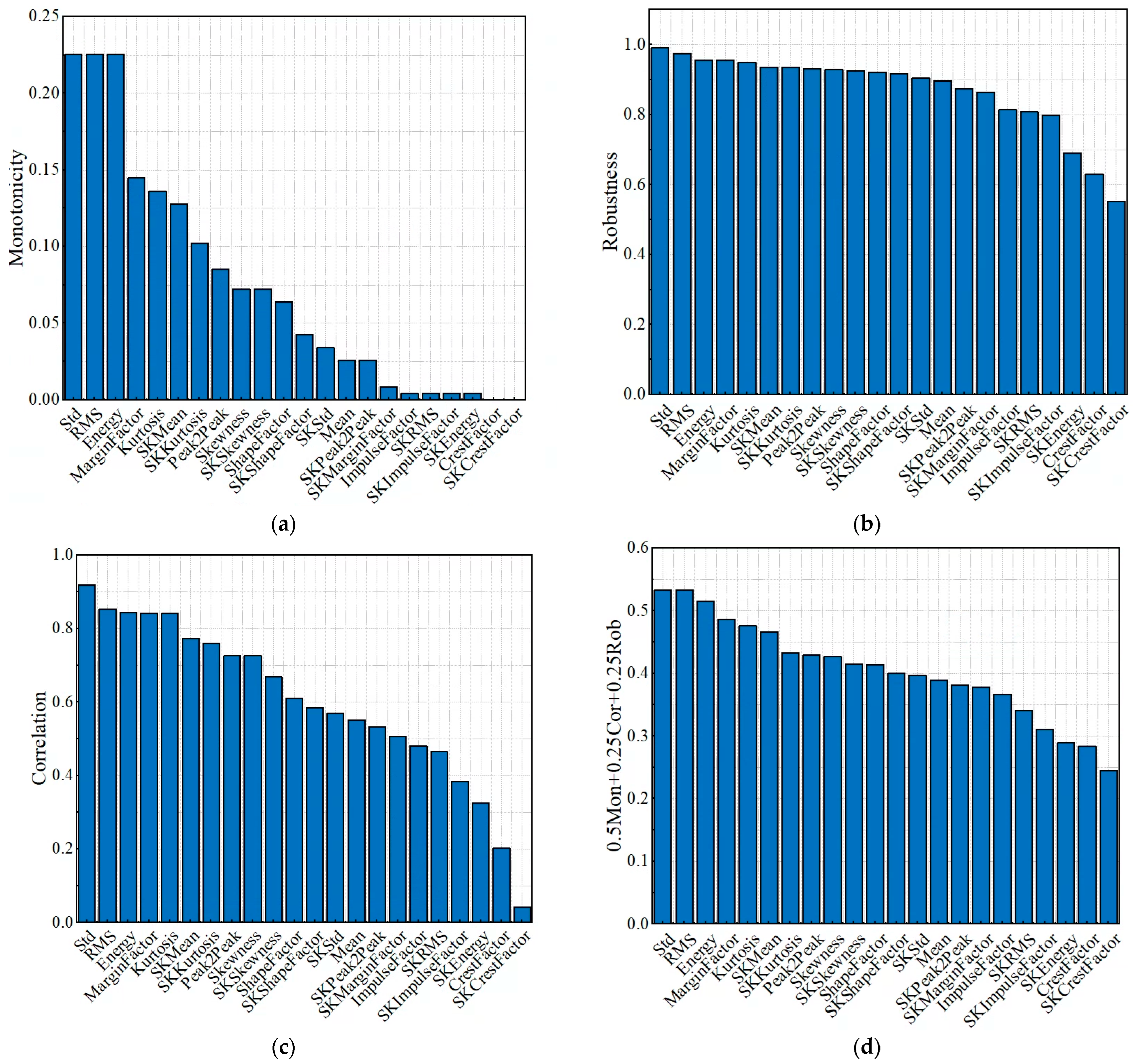
Here, CI is the ranking index of features, Ω is the set of evaluated features and ω i is the weight assigned to each feature evaluation indicator reflects its significance in the assessment. These weights are constrained within the range (0, 1). As bearing degradation progresses, damage accumulates, making the monotonicity of degradation features the utmost priority. Therefore, the weights of ω 1 = 0.25, ω 2 = 0.5, and ω 3 = 0.25 were chosen for C o r r Y , M o n Y , and R o b ( Y ) , respectively. With a data set of 3 bearing life cycles, performance calculations in the time domain and frequency domain were evaluated by the M o n Y ,   C o r r Y , and R o b ( Y ) indices as shown in Figure 2.
Figure 2 presents performance metrics for various attenuation indices, evaluating features in both the time and frequency domains using three different indices: monotonicity, robustness, and correlation. In Figure 2a, the monotonicity index reveals substantial variations in feature evaluation. In Figure 2b,c, the robustness and correlation metrics display little discernible distinction among the features. By aggregating all three indices, monotonicity, robustness, and correlation, with respective weights of 0.5, 0.25, and 0.25, we derive the feature evaluation results as shown in Figure 2d. Based on the insights from Figure 2d, we can select features such as Std, RMS, Energy, MarginFactor, Kurtosis, and SKMean to construct the HI.

2.2.3. PCA-Based HI Construction

The process of selecting optimal features in Section 2.2.2 distinctly reveals the degradation of the bearings for creating the HI. Principal Component Analysis (PCA) is a commonly employed technique for synthesizing data derived from the selected features, as discussed in [28]. PCA helps uncover the interaction patterns among features within sensitive feature sets. By means of orthogonal transformation, the original features are projected into a set of comprehensive features. Consequently, a reduced amount of data can effectively represent the primary informative features inherent in the input data, thereby achieving dimensionality reduction. The approach for constructing the HI based on PCA can be outlined in Figure 3:
The use of Z-score normalization method addresses the issue of disparate data weights arising from significant variations in the sizes of sensitive objects, enabling consistent treatment of input signals:
Y s t a n d a r d i z e d m × n = y i j m e a n ( y i j ) s t d ( y i j )     ,   i = 1,2 , 3 , m   j = 1,2 , 3 , n  
where Y s t a n d a r d i z e d m × n is the matrix of n selected features, m is the length of the features, m e a n y i j is the average value of each feature, and s t d y i j is the standard deviation of each feature.
The covariance matrix A for the Y s t a n d a r d i z e d m × n norm is determined:
A = i n ( y i j m e a n ( y i j ) ) ( y i j m e a n ( y i j ) ) T
Compute the eigenvalues λ and eigenvectors of the matrix A, the eigenvalues represent the variance of the first principal component, while the eigenvectors form the column vectors in the transformation matrix. The eigenvalues are arranged in ascending order, the largest eigenvalue λ is selected, and the corresponding eigenvector λ is used as a row vector to construct the eigenvector matrix B. After sorting the principal components, the subsequent step is to determine the number of dimensions to retain.
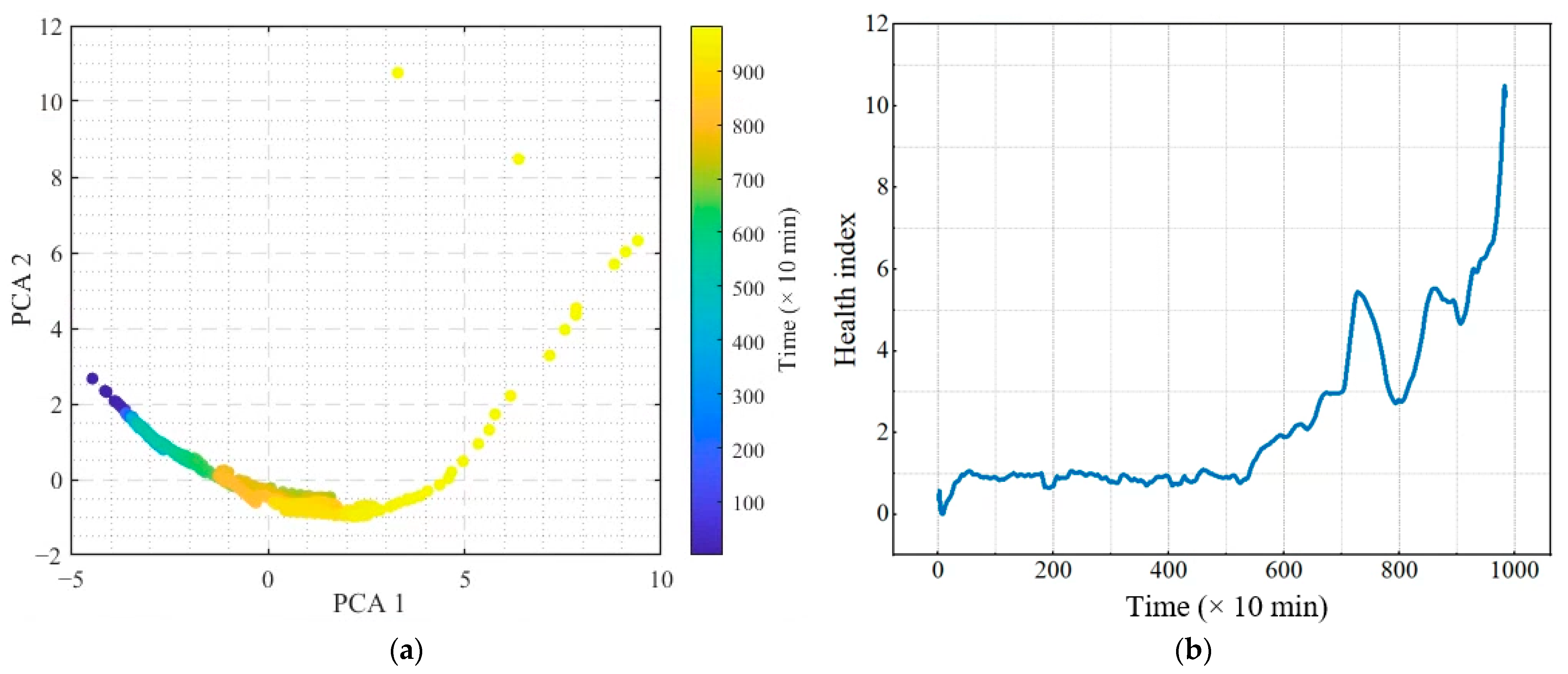
In this section, we use input including the top six features, Std, RMS, Energy, MarginFactor, Kurtosis, and SKMean. PCA analysis was conducted and the results are shown in Figure 4a. As depicted in Figure 4, it is clear that the PCA1 value gradually increases with the deterioration of the bearing. Therefore, PCA1 can be determined as a suitable HI for the bearing. Figure 4b shows the HI constructed through the PCA algorithm.

2.2.4. Outlier Region Correction

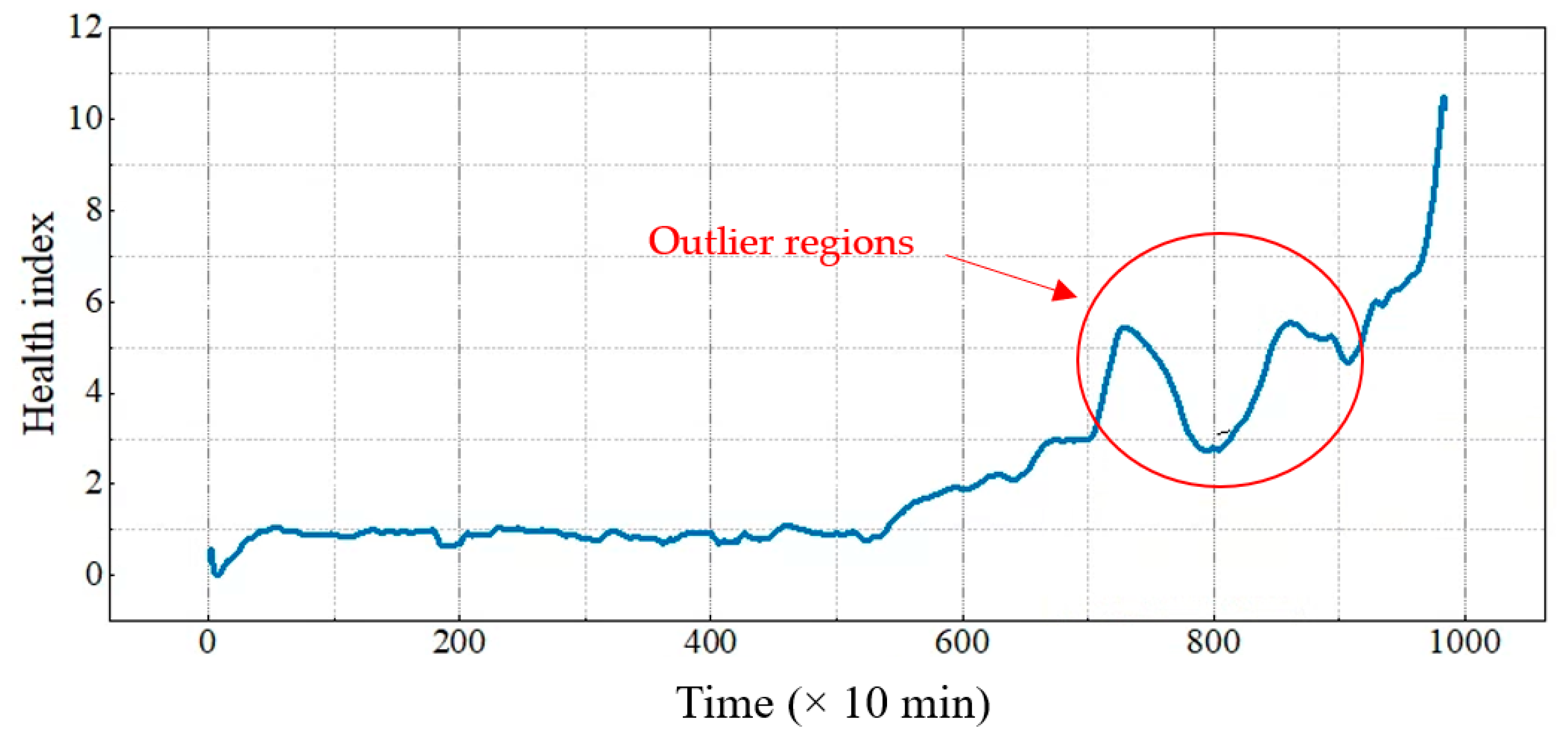
Just as described in Section 2.2.3, HI was constructed. However, as illustrated in Figure 5, the regions of fluctuation, marked within the circled rings, can complicate the RUL prediction model. The diagnostic performance is adversely affected as these regions do not conform to the bearing degradation pattern.
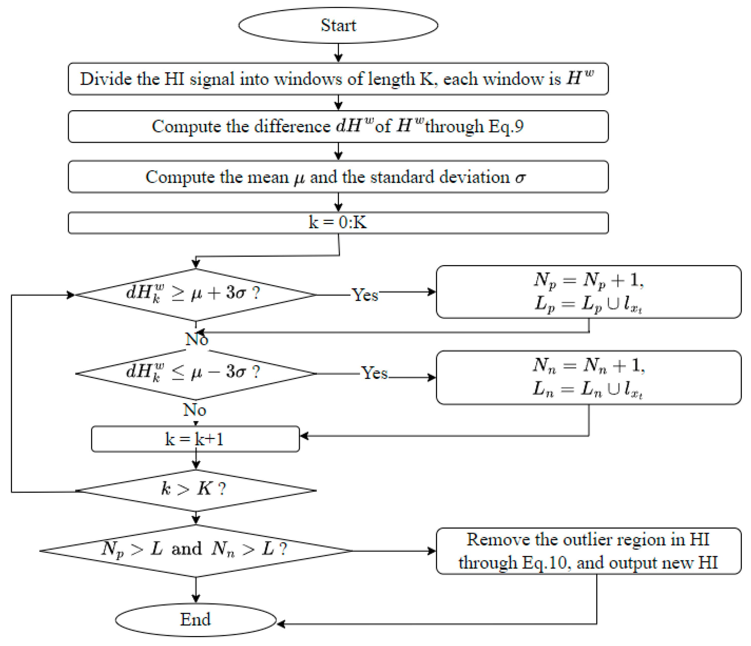
In this section, the objective is to eliminate the outlier regions from the HI to alleviate irregular trends. This correction process entails two fundamental steps: identifying outlier regions and removing them. As Liang Guo et al. mentioned in [29], the assumption that the generated HI exhibits a certain degree of increasing trend, signifying that deviations in the HI values remain within a specific range. Therefore, a method utilizing the 3 σ rule to identify outlier regions within the HI. Subsequently, the identified outlier regions are eliminated by connecting the starting point to the ending point of each respective outlier region. The detailed steps of this proposed outlier correction technique are outlined below as shown in Figure 6:
Here, N p , and N n are the number of positive outliers and negative outliers, respectively; L p   a n d   L n are the location set of the positive outliers and negative outliers.
In the stage of outlier region identification, the discrepancy in a HI is computed as follows:
d H k w = h k + 1 w h k w k
where h k w is the HI at the time k , and d H k w is the corresponding difference at time k .
The threshold for outlier detection is defined as:
T h r e s h o l d = μ + 3 σ ,   u p p e r   t h r e s h o l d   μ 3 σ ,       l o w e r   t h r e s h o l d
After identifying the outlier loop, eliminating the outlier region follows the following Formula (10):
h t c i = h t s w + h t e w h t s w t e t s ( t c t s )
where:
  • h t c i   is new HI when removing the outliers region
  • h t s c is HI at the time t s when the outlier region begins to appear.
  • h t e c   is HI at the time t e at the end of the exception region
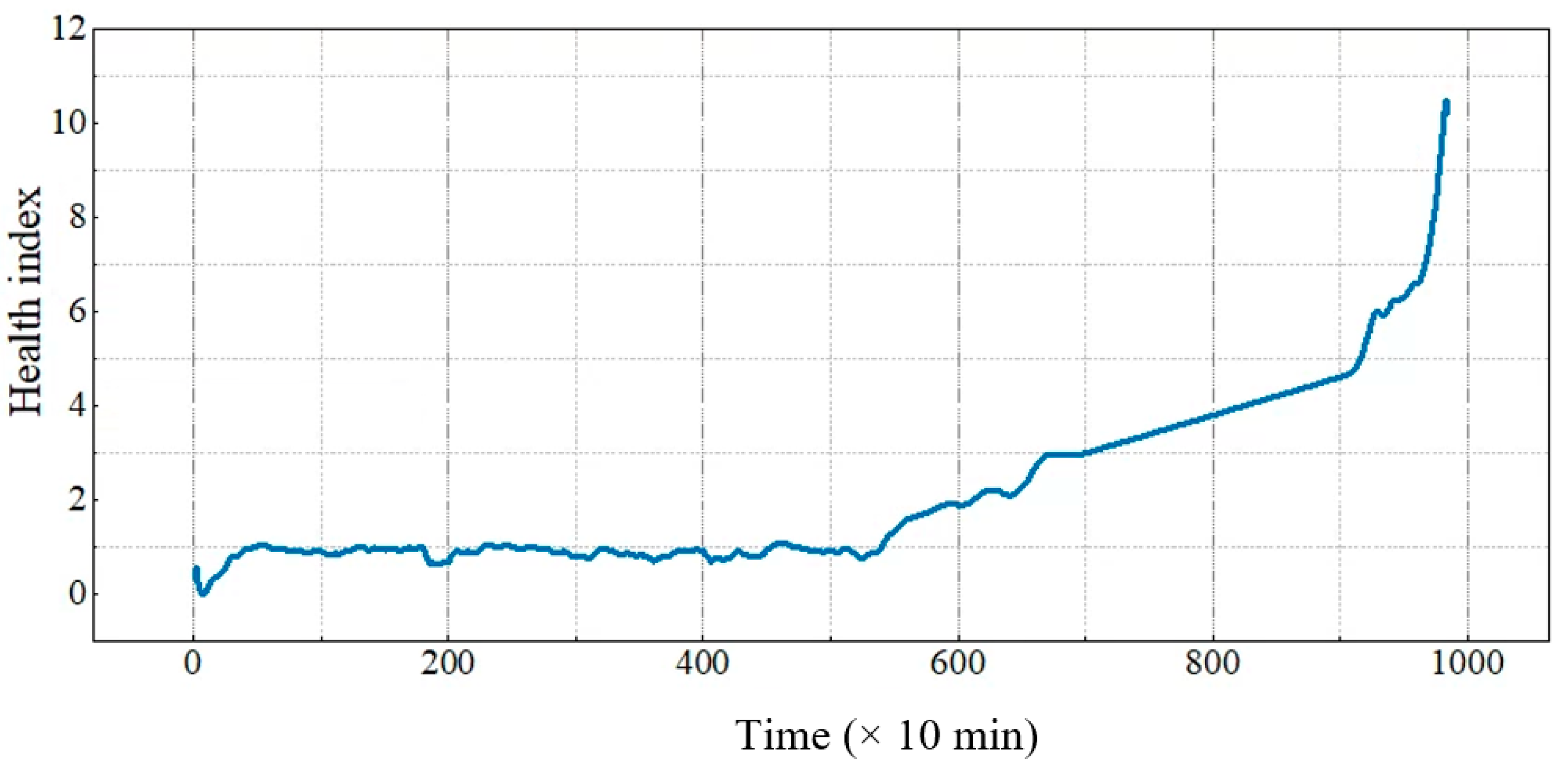
The HI built in Section 2.2.3 contains fluctuation regions and the above algorithm will be applied to process outlier regions and obtain a new HI as shown in Figure 7.

3. Designing a RUL Prediction Model Based on the HI

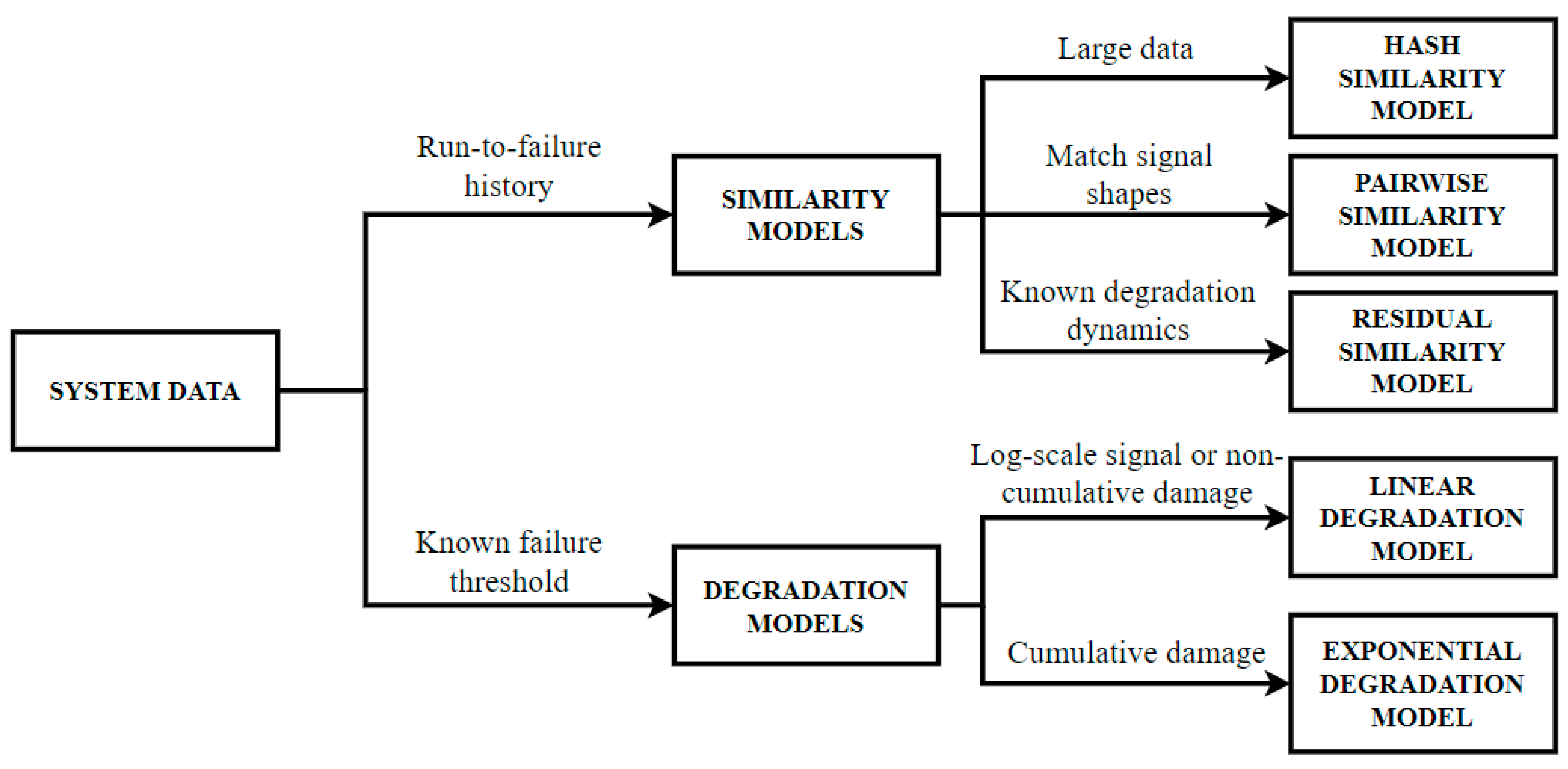
After completing the construction of the HI, two different approaches are compared: similarity modeling and degradation to predict bearing RUL based on the constructed HI and analyze their accuracy in terms of the data limitations as shown in Figure 8:

3.1. Similarity Models

Utilizing the dataset obtained from IMS, as described in Table 1, which comprises three data files reflecting the history of bearing performance until failure, we focus on the diagnosis of the remaining lifespan of the bearings. In this section, the process will involve the selection of a diagnostic model based on this dataset.
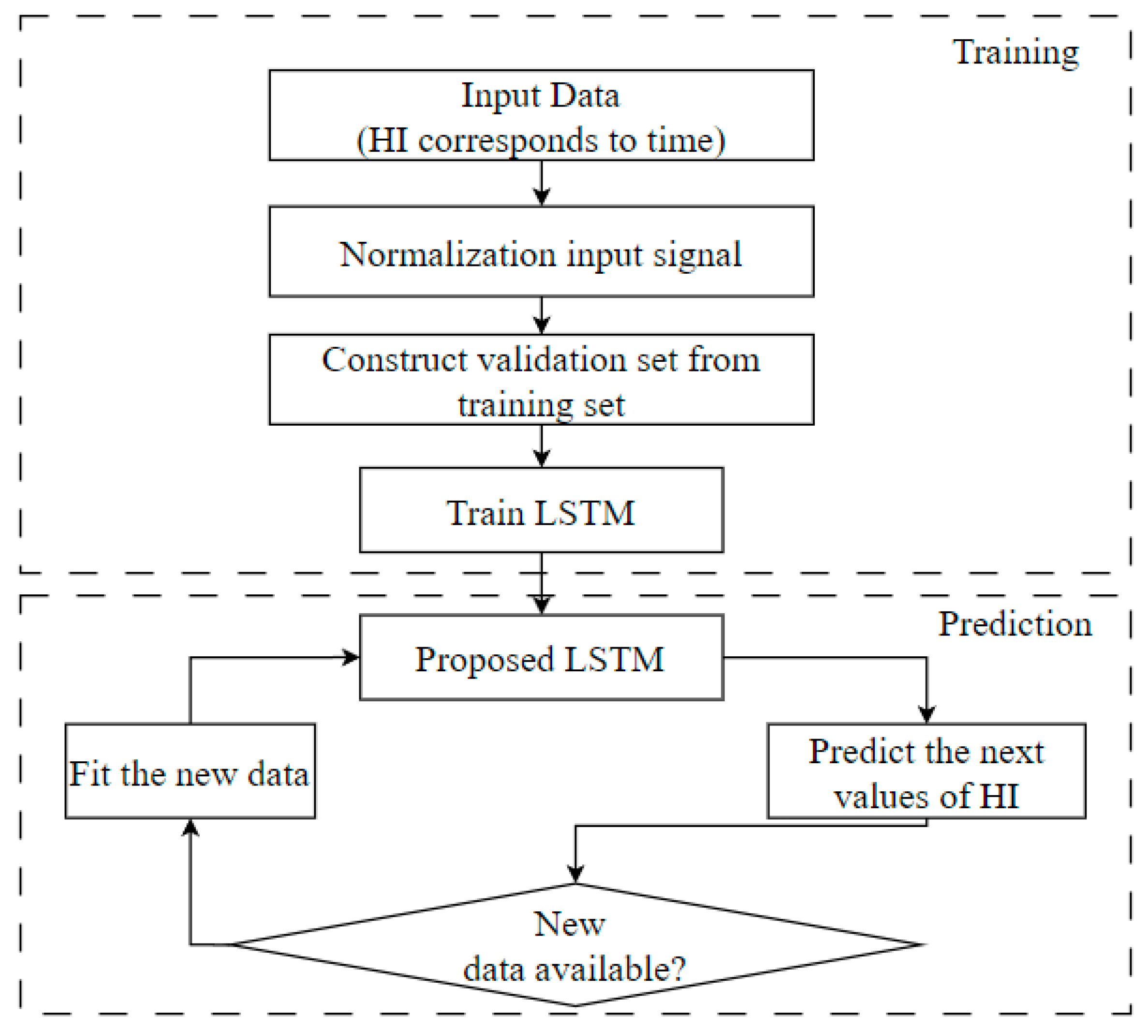
As illustrated in Figure 9, the predictive framework is primarily divided into three core components: data preprocessing, model training, and the prediction of RUL. Data preprocessing encompasses the creation of HI metrics, a process that has been comprehensively elucidated in Section 2. For model training, we opted for the LSTM model due to its specific design for handling time series data. This model excels in capturing temporal trends, intricate parameter interdependencies, and the ability to discern non-linear associations. LSTM possesses the capability to uncover such relationships, a task that conventional linear models struggle to achieve.

3.2. Degradation Models

By scrutinizing the characteristics of failures and conducting a thorough review of the literature [16], there are two distinct phases within the overall degradation process. In the initial stage, there is a gradual increase in the amplitude of vibration signals, followed by a rapid escalation in the second stage, ultimately culminating in the failure state within a brief timeframe. Consequently, apply specific regression models to the data in these two stages: a linear regression model for data representing slight degradation and an exponential model for data associated with severe degradation to efficiently and automatically pinpoint the moment of transition between degradation states. These thresholds are tailored to align with the performance of linear regression on windowed data, exponential regression on windowed data, and linear regression on observed data. The transition in degradation states is recognized when the threshold values of the linear regression models dip below 0.7 corresponding to the HI index built in Section 2.
The exponential model with random coefficients can be expressed in the following manner:
H t k = Φ + θ e β t k + ε σ 2 2
where, H t k signifies the HI value at time t k . Φ denotes the constant offsets determined by the linear regression model, as the inception point of the exponential model coincides with the termination point of the linear model. In addition, θ and β are stochastic parameters governing the model’s slope, where θ follows a lognormal distribution and β follows a Gaussian distribution. Finally, ϵ denotes Gaussian white noise, motion with a mean of μ = 0 and a variance of σ2.

3.3. RUL Prediction Results

  • Similarity Models
Using a dataset comprising results from three experiments of the run-to-fail circuit and the calculation of the HI as described in Section 3.1, the LSTM model is trained on two out of the three HI values and tested on the remaining dataset. The LSTM model configuration is specified in Table 3, and the outcomes are presented in Figure 10.
Figure 10 indicates a smooth transition to the final rise of HI for bearing 1, while bearings 2 and 3, respectively show fluctuations and predict failure to reach the error threshold of HI value, with a set HI failure threshold of 10, only the first case reaches this limit. Consequently, the LSTM model fails to capture the rapidly rising trend of HI during the severe degradation stage. This limitation arises from the small input dataset, hindering the model’s ability to learn the deterioration trend of the bearings.
b.
Degradation Models
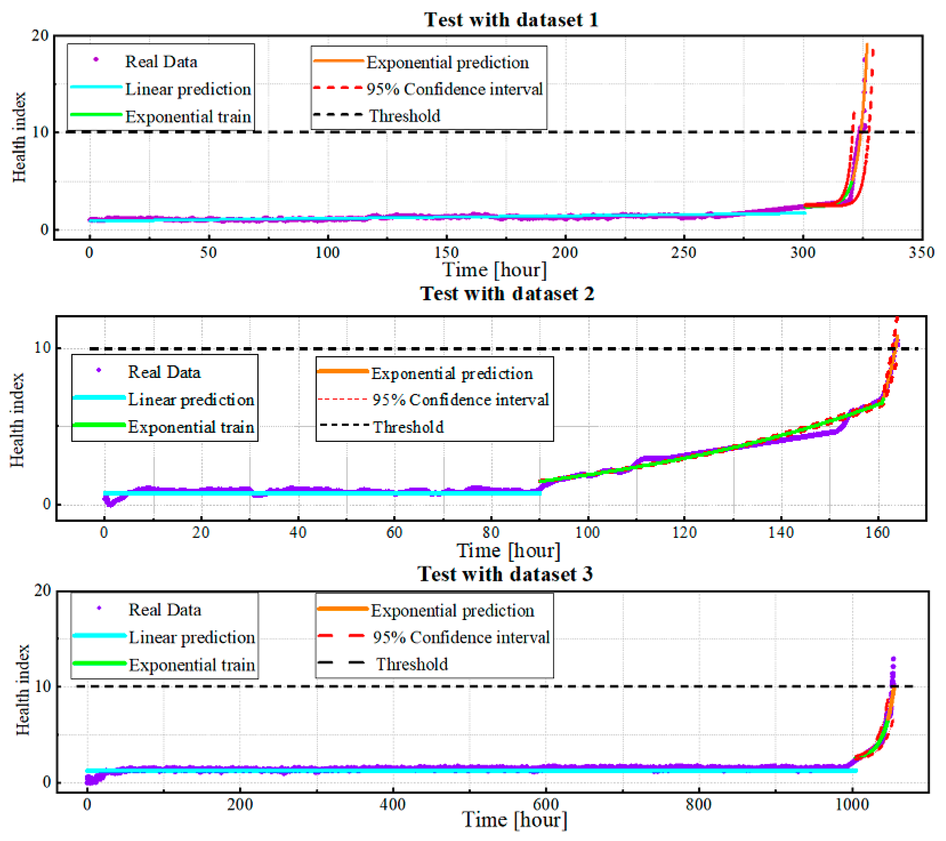
Based on the degradation models presented in Section 3.2, predictions are made for three failure cases in the data set of Section 2. After adjusting each value of the threshold, the mild and severe deterioration stages of HI data are adjusted using linear regression and a stochastic exponential random coefficient model, respectively. For each case, the appropriate real-time RUL prediction models are updated by incorporating the newly discovered data points, and future HI is predicted for the next 10 h.
The automatic threshold setting from the linear region to the degradation region is 0.7. Figure 11 shows that the RUL prediction results closely follow the actual data. In the three HI prediction cases, 3 cases all reach the bearing failure threshold set at 10. Therefore, the model proposed in Section 3.2 is said to give acceptable prediction results for bearings based on vibration data.
c.
Discussions
Three HIs sets were created from the raw data, and an LSTM model was trained using two of these sets and then tested on the third. Testing outcomes, depicted in Figure 10, show that while Bearing 1 transitions smoothly to the final HI rise, Bearings 2 and 3 display initial and pre-final oscillations. This suggests the LSTM model’s failure to detect the swift HI increase during critical deterioration. Regarding the proposed degradation model, it accurately predicted three failure cases, adapting real-time RUL prediction models by integrating new data points, thereby forecasting future HI. Figure 11 illustrates satisfactory prediction results for all three bearings when HI reaches the threshold. In the context of similarity models, having the most suitable data for model training is essential. The challenge of acquiring comprehensive run-to-failure datasets, especially for wind turbines with long service lives, limits the full potential of similarity model training and performance. In practice, obtaining run-to-failure datasets, particularly for wind turbines with a service life of up to 20 years, can be challenging. To address this, degradation models use bearing datasets running until the desired time of diagnosis, enabling precise RUL predictions within a feasible timeframe and providing a more thorough understanding of bearing damage compared with LSTM-based similarity models in RUL prediction. The accurate RUL prediction in this study enhances the proposed wind turbine condition monitoring system’s ability to collect real-time data and predict the RUL of component wind turbines using vibration signals. These predictions are relayed to operators as valuable references for conducting predictive maintenance, pre-empting severe turbine failures. This approach not only reduces downtime through proactive planning for component supply and repair but also minimizes damage to adjacent components. Consequently, this method is expected to bolster the operational reliability of offshore wind turbines and enable cost-effective maintenance via condition monitoring systems.

4. Conclusions

This paper has delved into the critical imperative of addressing the issue of RUL prediction for key components in wind turbines, particularly focusing on vibration signals. The proposed prognostic method, focusing on constructing a comprehensive bearing HI, stands out as a novel contribution. By integrating feature selection, outlier elimination, and two distinct RUL prediction approaches, the method aims to enhance accuracy and reduce model complexity. The results, as demonstrated by the comparison of the two models’ similarity and degradation using the same dataset, indicate that the degradation model outperforms, offering superior prognostic results and proving more suitable for contemporary wind turbines. The article introduces a unique perspective on the challenges of RUL prediction, highlighting the importance of selecting appropriate methodologies based on specific application contexts. This insight not only advances the field of prognostic methods for wind turbine components but also underscores the broader implications for optimizing maintenance processes, mitigating downtime, and improving overall system availability. Looking ahead, the future plan involves refining and expanding the proposed methodology to account for evolving technological landscapes and emerging challenges in the renewable energy sector. Ongoing research efforts will focus on incorporating real-time data streams, machine learning advancements, and continuous model improvement. The aim is to develop a more robust and adaptive prognostic framework that can effectively address the dynamic nature of wind turbine operations. As industries grapple with the need for sustainable energy solutions, the insights presented in this article provide valuable guidance for practitioners and researchers alike, fostering a deeper understanding of the intricacies involved in predictive maintenance strategies for renewable energy systems such as wind turbines.

Author Contributions

Conceptualization and methodology, T.-T.L. and M.-C.D.; software, T.-T.L.; validation, T.-T.L. and M.-C.D.; investigation, T.-T.L. and M.-C.D.; writing—original draft preparation, T.-T.L.; writing—review and editing, T.-T.L. and M.-C.D.; project administration, S.-J.L.; supervision, M.P. All authors have read and agreed to the published version of the manuscript.

Funding

This work was supported by the Korea Institute of Energy Technology Evaluation and Planning (KETEP) grant funded by the Korea government (MOTIE) (20223030020180). Development of durability evaluation and remaining useful life prediction technology for wind turbine life extension.

Data Availability Statement

Data are contained within the article.

Conflicts of Interest

The authors declare no conflict of interest.

Abbreviations

COECost of Energy
IMSIntelligent Maintenance Systems
IAEInternational Energy Agency
IEAInternational Energy Agency
RULRemaining Useful Life
HIHealth Index
PCAPrincipal Component Analysis
LSTMLong Short-term Memory
RMSRoot Mean Square
SVMSupport Vector Machine
RNNRecurrent Neural Networks

References

  1. Li, L.; Lin, J.; Wu, N.; Xie, S.; Meng, C.; Zheng, Y.; Wang, X.; Zhao, Y. Review and outlook on the international renewable energy development. Energy Built Environ. 2022, 3, 139–157. [Google Scholar] [CrossRef]
  2. IRENA. Renewable Electricity Capacity and Generation Statistics; IRENA: Abu Dhabi, United Arab Emirates, 2018. [Google Scholar]
  3. Rubanenko, O.; Miroshnyk, O.; Shevchenko, S.; Yanovych, V.; Danylchenko, D.; Rubanenko, O. Distribution of wind power generation dependently of meteorological factors. In Proceedings of the 2020 IEEE KhPI Week on Advanced Technology (KhPIWeek), Kharkiv, Ukraine, 5–10 October 2020; pp. 472–477. [Google Scholar]
  4. Transformation, Global Energy. Global Energy Transformation: A Roadmap to 2050; Transformation, Global Energy: Abu Dhabi, United Arab Emirates, 2018. [Google Scholar]
  5. El-Thalji, I.; Jantunen, E. On the development of condition based maintenance strategy for offshore wind farm: Requirement elicitation process. Energy Procedia 2012, 24, 328–339. [Google Scholar] [CrossRef]
  6. Park, J.; Kim, C.; Dinh, M.-C.; Park, M. Design of a Condition Monitoring System for Wind Turbines. Energies 2022, 15, 464. [Google Scholar] [CrossRef]
  7. Ben-Daya, M.; Duffuaa, S.O.; Raouf, A.; Knezevic, J.; Ait-Kadi, D. Handbook of Maintenance Management and Engineering; Springer: Berlin/Heidelberg, Germany, 2009; Volume 7. [Google Scholar]
  8. Kandukuri, S.T.; Klausen, A.; Karimi, H.R.; Robbersmyr, K.G. A review of diagnostics and prognostics of low-speed machinery towards wind turbine farm-level health management. Renew. Sustain. Energy Rev. 2016, 53, 697–708. [Google Scholar] [CrossRef]
  9. Nielsen, J.S.; Sørensen, J.D.; Abrahamsen, A.B.; Kolios, A. IEA Wind Task 42: Lifetime Extension Assessment, Deliverable Report 3+7: RECOMMENDATIONS on Standards and Regulatory Frame. October 2022. Available online: https://iea-wind.org/wp-content/uploads/2023/06/Task-42-report-D37_RecommendationStandardsRegulatoryFrame-v3.pdf (accessed on 1 October 2023).
  10. Bolander, N.; Qiu, H.; Eklund, N.; Hindle, E.; Rosenfeld, T. Physics-based remaining useful life prediction for aircraft engine bearing prognosis. In Proceedings of the Annual Conference of the PHM Society, San Diego, CA, USA, 27 September–1 October 2009. [Google Scholar]
  11. Ning, Y.; Wang, G.; Yu, J.; Jiang, H. A feature selection algorithm based on variable correlation and time correlation for predicting remaining useful life of equipment using rnn. In Proceedings of the 2018 Condition Monitoring and Diagnosis (CMD), Perth, WA, Australia, 23–26 September 2018; pp. 1–6. [Google Scholar]
  12. Ahmad, W.; Khan, S.A.; Islam, M.M.; Kim, J.M. A reliable technique for remaining useful life estimation of rolling element bearings using dynamic regression models. Reliab. Eng. Syst. Saf. 2019, 184, 67–76. [Google Scholar] [CrossRef]
  13. Ahmad, W.; Khan, S.A.; Kim, J.M. A hybrid prognostics technique for rolling element bearings using adaptive predictive models. IEEE Trans. Ind. Electron. 2017, 65, 1577–1584. [Google Scholar] [CrossRef]
  14. Duan, L.; Zhao, F.; Wang, J.; Wang, N.; Zhang, J. An integrated cumulative transformation and feature fusion approach for bearing degradation prognostics. Shock. Vib. 2018, 2018, 9067184. [Google Scholar] [CrossRef]
  15. Yan, M.; Wang, X.; Wang, B.; Chang, M.; Muhammad, I. Bearing remaining useful life prediction using support vector machine and hybrid degradation tracking model. ISA Trans. 2020, 98, 471–482. [Google Scholar] [CrossRef] [PubMed]
  16. Dataset, N.B. NASA Bearing Dataset: Prognostic Dataset for Predictive/Preventive Maintenance. Available online: https://www.kaggle.com/datasets/vinayak123tyagi/bearing-dataset?fbclid=IwAR0FRT1RwK05uDNetsPdahy5JhxGWiE81YhAJiA9dP386bySdXkPq6k2kAo (accessed on 1 July 2023).
  17. Wymore, M.L.; Van Dam, J.E.; Ceylan, H.; Qiao, D. A survey of health monitoring systems for wind turbines. Renew. Sustain. Energy Rev. 2015, 52, 976–990. [Google Scholar] [CrossRef]
  18. Tandon, N.; Choudhury, A. A review of vibration and acoustic measurement methods for the detection of defects in rolling element bearings. Tribol. Int. 1999, 32, 469–480. [Google Scholar] [CrossRef]
  19. Antoni, J.; Randall, R.B. The spectral kurtosis: Application to the vibratory surveillance and diagnostics of rotating machines. Mech. Syst. Signal Process. 2006, 20, 308–331. [Google Scholar] [CrossRef]
  20. Ali, J.B.; Chebel-Morello, B.; Saidi, L.; Malinowski, S.; Fnaiech, F. Accurate bearing remaining useful life prediction based on Weibull distribution and artificial neural network. Mech. Syst. Signal Process. 2015, 56, 150–172. [Google Scholar]
  21. Obeid, Z.; Picot, A.; Poignant, S.; Régnier, J.; Darnis, O.; Maussion, P. Experimental comparison between diagnostic indicators for bearing fault detection in synchronous machine by spectral Kurtosis and energy analysis. In Proceedings of the IECON 2012—38th Annual Conference on IEEE Industrial Electronics Society, Montreal, QC, Canada, 25–28 October 2012; pp. 3901–3906. [Google Scholar]
  22. Antoni, J. The spectral kurtosis: A useful tool for characterising non-stationary signals. Mech. Syst. Signal Process. 2006, 20, 282–307. [Google Scholar] [CrossRef]
  23. Zhang, B.; Zhang, L.; Xu, J. Degradation feature selection for remaining useful life prediction of rolling element bearings. Qual. Reliab. Eng. Int. 2016, 32, 547–554. [Google Scholar] [CrossRef]
  24. Li, N.; Lei, Y.; Lin, J.; Ding, S.X. An improved exponential model for predicting remaining useful life of rolling element bearings. IEEE Trans. Ind. Electron. 2015, 62, 7762–7773. [Google Scholar] [CrossRef]
  25. Yang, F.; Habibullah, M.S.; Zhang, T.; Xu, Z.; Lim, P.; Nadarajan, S. Health index-based prognostics for remaining useful life predictions in electrical machines. IEEE Trans. Ind. Electron. 2016, 63, 2633–2644. [Google Scholar] [CrossRef]
  26. Li, N.; Lei, Y.; Liu, Z.; Lin, J. A particle filtering-based approach for remaining useful life predication of rolling element bearings. In Proceedings of the 2014 International Conference on Prognostics and Health Management, Cheney, WA, USA, 22–25 June 2014; pp. 1–8. [Google Scholar]
  27. Javed, K.; Gouriveau, R.; Zerhouni, N.; Nectoux, P. Enabling health monitoring approach based on vibration data for accurate prognostics. IEEE Trans. Ind. Electron. 2014, 62, 647–656. [Google Scholar] [CrossRef]
  28. Mosallam, A.; Medjaher, K.; Zerhouni, N. Data driven prognostic method based on Bayesian approaches for direct remaining useful life prediction. J. Intell. Manuf. 2016, 27, 1037–1048. [Google Scholar] [CrossRef]
  29. Guo, L.; Lei, Y.; Li, N.; Yan, T.; Li, N. Machinery health indicator construction based on convolutional neural networks considering trend burr. Neurocomputing 2018, 292, 142–150. [Google Scholar] [CrossRef]
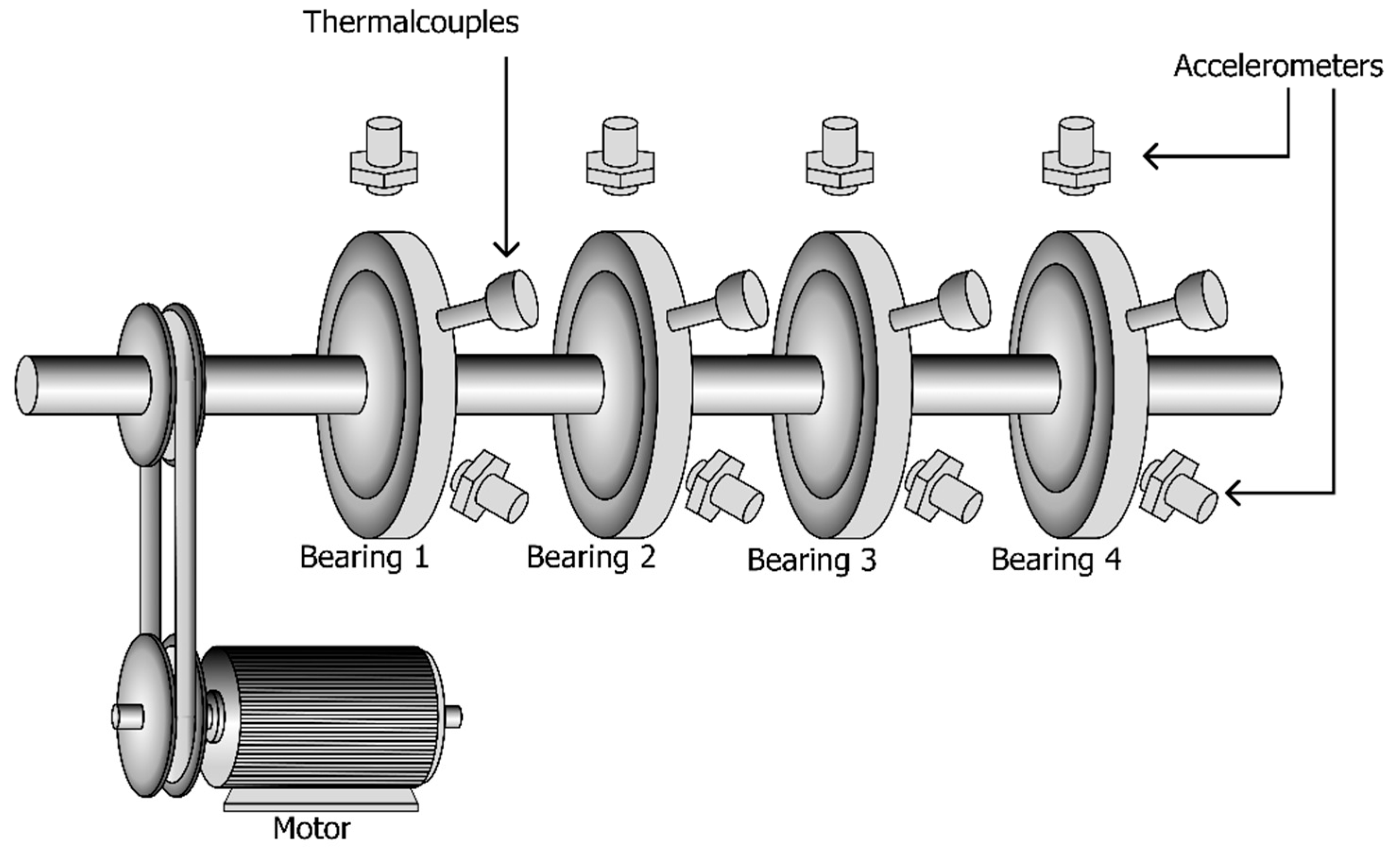
Figure 1. Bearing test rig.
Energies 17 00019 g001
Figure 2. Indices performance metrics: (a) Monotonicity; (b) robustness; (c) correlation; (d) 0.5 Mon + 0.25 Corr + 0.25 Rob.
Energies 17 00019 g002
Figure 3. The process of determining HI from PCA.
Energies 17 00019 g003
Figure 4. (a) The principal component; (b) HI was built from features selected.
Energies 17 00019 g004
Figure 5. The HI value has not been eliminated from the outlier.
Energies 17 00019 g005
Figure 6. Flowchart for the algorithm to eliminate outliers in the HI.
Energies 17 00019 g006
Figure 7. The HI value has been eliminated from the outlier.
Energies 17 00019 g007
Figure 8. Approach to predicting RUL of main bearing.
Energies 17 00019 g008
Figure 9. The process of diagnosing the RUL of the device is based on the similarity model.
Energies 17 00019 g009
Figure 10. RUL prediction results of similarity models.
Energies 17 00019 g010
Figure 11. RUL prediction results of degradation models.
Energies 17 00019 g011
Table 1. Details of the data set.
CaseRecording DurationNo. of FilesDescription
Set No. 122 October 2003 12:06:24 to 25 November 2003 23:39:562156
(8 channels)
At the end of the test-to-failure experiment, inner race defect occurred in bearing 3 and roller element defect in bearing 4.
Set No. 212 February 2004 10:32:39 to 19 February 2004 06:22:39984
(4 channels)
At the end of the test-to-failure experiment, outer race failure occurred in bearing 1
Set No. 34 March 2004 09:27:46 to 4 April 2004 19:01:574448
(4 channels)
At the end of the test-to-failure experiment, outer race failure occurred in bearing 3
Table 2. Features in the time domain are extracted.
FeatureFormula
Mean y ¯ = 1 N i = 1 N y i
Standard deviation σ = 1 N i = 1 N y i y ¯ 1 2
Skewness 1 N i = 1 N y i y ¯ 3 ρ 3
Kurtosis 1 N i = 1 N y i y ¯ 4 ρ 4
Peak to Peak y m a x y m i n
Root mean square (RMS) R M S = 1 N i = 1 N y i 2 1 2
Crest factor y m a x R M S
Shape factor R M S 1 N i = 1 N y i
Impulse factor y m a x 1 N i = 1 N y i
Margin factor y m a x 1 N i = 1 N y i 2
Energy i = 1 N y i 2
Table 3. LSTM model configuration.
AI ModelParameters
AI model node1024 LSTM
Activation functionSigmoid
Epoch100
Batch size120
OptimizerAdam
Drop output0.5
Disclaimer/Publisher’s Note: The statements, opinions and data contained in all publications are solely those of the individual author(s) and contributor(s) and not of MDPI and/or the editor(s). MDPI and/or the editor(s) disclaim responsibility for any injury to people or property resulting from any ideas, methods, instructions or products referred to in the content.