Article

Enhancing LOCA Breach Size Diagnosis with Fundamental Deep Learning Models and Optimized Dataset Construction

1
Institute of Nuclear and New Energy Technology, Tsinghua University, Beijing 100084, China
2
Research Institute of Macro-Safety Science, University of Science and Technology Beijing, Beijing 100083, China
3
School of Computer Science and Technology, University of Chinese Academy of Sciences, Beijing 100049, China
*
Author to whom correspondence should be addressed.
These authors contributed equally to this work.
Energies 2024, 17(1), 159; https://doi.org/10.3390/en17010159
Submission received: 19 October 2023 / Revised: 14 December 2023 / Accepted: 16 December 2023 / Published: 27 December 2023
(This article belongs to the Special Issue Nuclear and New Energy Technology)

Abstract

:
In nuclear power plants, the loss-of-coolant accident (LOCA) stands out as the most prevalent and consequential incident. Accurate breach size diagnosis is crucial for the mitigation of LOCAs, and identifying the cause of an accident can prevent catastrophic consequences. Traditional methods mostly focus on combining model algorithms and utilize intricate composite model neural network architectures. However, it is crucial to investigate whether greater complexity necessarily leads to better performance. In addition, the consideration of the impact of dataset construction and data preprocessing on model performance is also needed for model building. This paper proposes a framework named DeepLOCA-Lattice to experiment with different preprocessing approaches to fundamental deep learning models for a comprehensive analysis of the diagnosis of LOCA breach size. The DeepLOCA-Lattice involves data preprocessing via the lattice algorithm and equal-interval partitioning and deep-learning-based models, including the multi-layer perceptron (MLP), recurrent neural networks (RNNs), convolutional neural networks (CNNs), and the transformer model in LOCA breach size diagnosis. After conducting rigorous ablation experiments, we have discovered that even rudimentary foundational models can achieve accuracy rates that exceed 90%. This is a significant improvement when compared to the previous models, which yield an accuracy rate of lower than 50%. The results interestingly demonstrate the superior performance and efficacy of the fundamental deep learning model, with an effective dataset construction approach. It elucidates the presence of a complex interplay among diagnostic scales, sliding window size, and sliding stride. Furthermore, our investigation reveals that the model attains its highest accuracy within the discussed range when utilizing a smaller sliding stride size and a longer sliding window length. This study could furnish valuable insights for constructing models for LOCA breach size estimation.

1. Introduction

Nuclear power plants (NPPs) consist of multiple intricate, nonlinear, and dynamic systems. The availability of large amounts of information from operators, due to advances in digital technology [1], has made it challenging to swiftly diagnose fault information. Furthermore, research has established human error as the primary cause of accidents in NPPs [2], in particular, the intrinsic human factors of uncertainty [3] and the impact of human–computer interface design [4]. To ensure safe operations, minimize the impact of human factors during accidents, and mitigate economic losses, automating the precise and accurate recognition of fault information in NPPs is crucial.
A loss-of-coolant accident (LOCA) is a prevalent type of mishap in nuclear power plants, posing significant potential hazards. As shown in Figure 1, the LOCA originates from a leakage in the reactor system, which causes the coolant to escape and leaves the reactor vulnerable to high temperatures and subsequent damage [5]. The severity of the LOCA varies depending on the size of the breach, which requires customizing emergency measures accordingly. Consequently, estimating the breach size of the LOCA is a crucial step in accident response planning, as it provides essential information for determining appropriate emergency response actions. Neural network models have emerged as an effective and popular strategy for describing accident behavior [6]. Therefore, in this study, our aim is to thoroughly investigate the performance metrics of fundamental neural networks within the domain of deep learning. The names and abbreviations of the primary parameters in this article are shown in Table 1.
The rest of the paper is organized as follows: Section 2 introduces the related work. Section 3 contains relevant concepts, and Section 4 details the DeepLOCA-Lattice adopted for LOCA breach size diagnosis. Section 5 presents scenario deduction and sensitivity analysis, and Section 6 provides the discussion and conclusions.

2. Related Work

With the progress of deep learning (DL), several hybrid models composed of multiple deep learning models for diagnosis have been successfully applied in the nuclear fault diagnosis field [7]. As shown in Table 2, She et al. combined CNN, LSTM, and convolutional LSTM (ConvLSTM) for the diagnosis and prediction of LOCAs, and this hybrid model has been proven to be functional, accurate, and divisible [8]. Meanwhile, Choi et al. used a cascaded fuzzy neural network (CFNN) to estimate the size of the LOCA breach [9]. Furthermore, Wang et al. proposed a PKT algorithm to extract more general fault information for NPP fault diagnosis and construct the coarse-to-fine knowledge structure intelligently [10], while Mandal et al. applied a deep belief network (DBN) to classify fault data in an NPP [11]. Yao et al. optimized convolutional neural networks with small-batch-size processing for assembly in the NPP diagnostic system [12], and Wang et al. presented a highly accurate and adaptable fault diagnosis technique based on the convolutional gated recurrent unit (CGRU) and improved particle swarm optimization (EPSO) [13]. Saghafi et al. defined a type of recurrent neural network model known as a nonlinear auto-regressive model with exogenous input (NARX) for LOCA breach size diagnosis [14]. However, there exists a significant complexity within the models used in prior research. The exploration of simpler, fundamental models for the accurate diagnosis of loss-of-coolant accident (LOCA) faults has not yet been undertaken.
In various domains, there is work leveraging deep learning for the purpose of assimilating data from monitoring points to forecast critical parameters. Xu et al. [15] presented, in the form of the transfer learning framework based on transformer (TL-Transformer), an accurate prediction of flooding in data-sparse basins. El-Shafeiy et al. [16] introduced and applied a pioneering technology, multivariate multiple convolutional networks with long short-term memory (MCN-LSTM), to real-time water quality monitoring. Liapis et al. [17] used deep learning in conjunction with models that extract emotion-related information from text to predict financial time series. Islam et al. [18] presented a combined architecture of a convolutional neural network (CNN) and recurrent neural network (RNN) to diagnose COVID-19 patients from chest X-rays.
In addressing the critical challenge of LOCAs in nuclear power plants, our research marks a significant departure from traditional, complex neural network architectures towards a more streamlined methodology. Previous studies, such as those by She et al. [8] and Choi et al. [9], have predominantly employed intricate, composite models. While these models are effective, they often require substantial computational resources and a deep understanding of varied neural network configurations.
Our study, in contrast, explores the untapped capabilities of fundamental neural network models, illustrating that simplicity can coexist with high accuracy. We have methodically developed and applied a simplified neural network model that, despite its reduced complexity, achieves an accuracy rate over 90%. This not only questions the prevailing dependence on complex models in LOCA fault diagnosis but also offers a more accessible and efficient alternative.
This research fills a vital gap in the literature, demonstrating that a well-designed, simpler model can match or even outperform complex systems. This is of paramount importance in the high-stakes environment of nuclear power plant operations, where rapid and reliable diagnostics are crucial. Simplifying the model structure also increases the interpretability and user-friendliness, making it more viable for practical applications, especially in settings with limited resources and expertise.
Additionally, previous research has focused primarily on combining model algorithms, with little consideration given to the impact of dataset construction and data preprocessing on model performance. To avoid the issues mentioned above, we propose a framework named DeepLOCA-Lattice for integrated analysis of LOCA breach size diagnosis. This framework has the potential to expand the scope of fault severity diagnosis for other types of accidents in NPPs. Furthermore, note that there are few studies on the high-precision diagnosis of LOCA breach size. Only the cascaded fuzzy neural networks proposed by Choi et al. [9] in 2016 and the NARX neural network suggested by Saghafi et al. [14] in 2019 are known to the authors.

3. Methodology

3.1. Structure of Proposed DeepLOCA-Lattice Framework

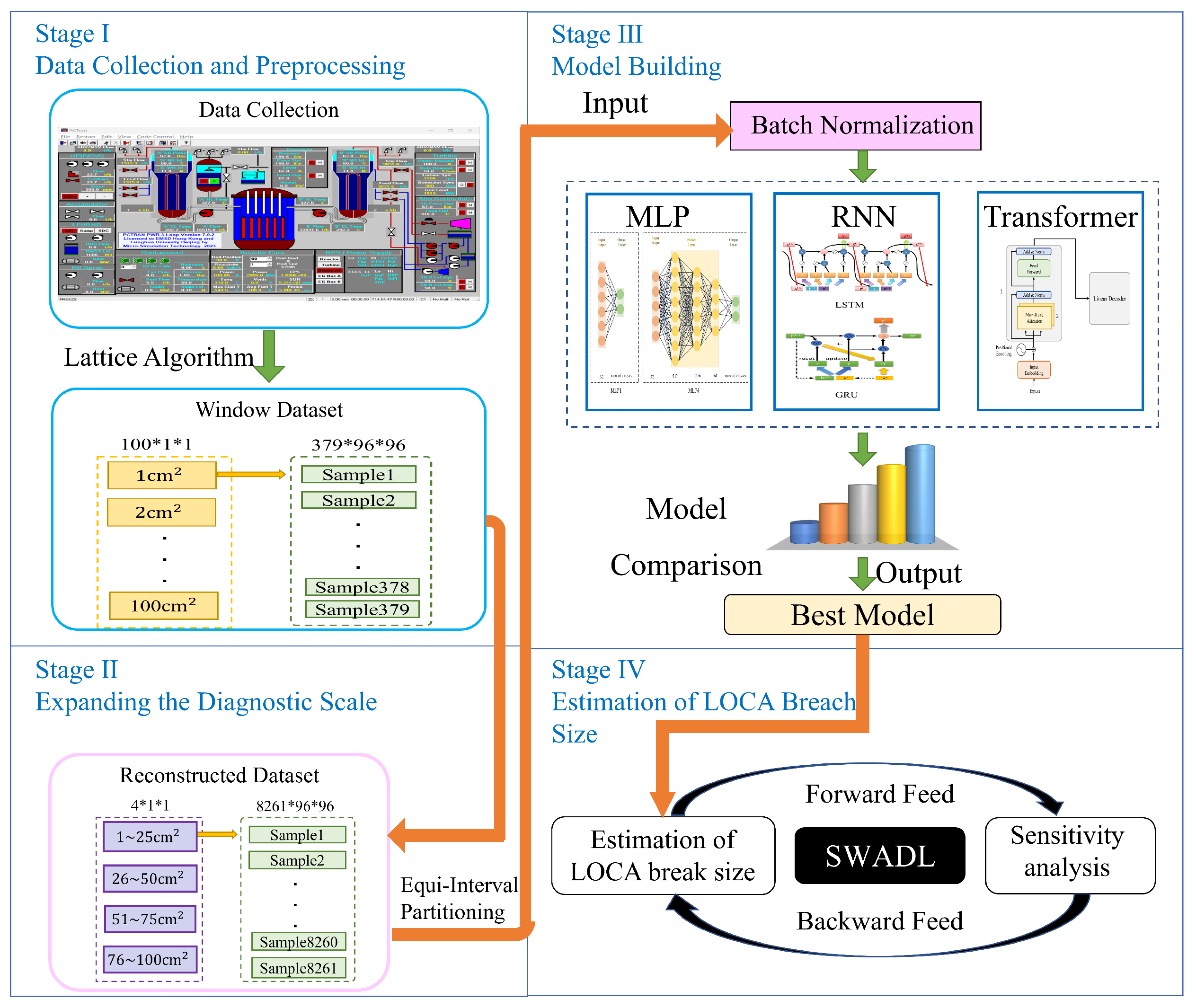
As illustrated in the flow diagram in Figure 2, the proposed DeepLOCA-Lattice framework consists of four main stages: data collection and preprocessing, expanding the diagnostic scale, model building, and estimation of the size of LOCA breaches. In the data preprocessing stage, the lattice algorithm is used to segment the original data into smaller windows, allowing the capture of temporal dependencies between data samples and the extraction of meaningful features for classification. After data preprocessing, four classes are defined based on the size of the LOCA breach using an equal-interval partitioning approach for expanding the diagnostic scale. For stage III, we experimented with five different deep learning models for the estimation of the LOCA breach size and the detection of key factors for the estimation model, namely, the simplified MLP, MLP, LSTM, GRU, CNN, and transformer models. Lastly, in a nuclear power plant during normal operation, if a LOCA incident occurs, the parameters from various sensors are input into our model, enabling the specific LOCA breach sizes to be estimated.

3.2. Lattice Algorithm

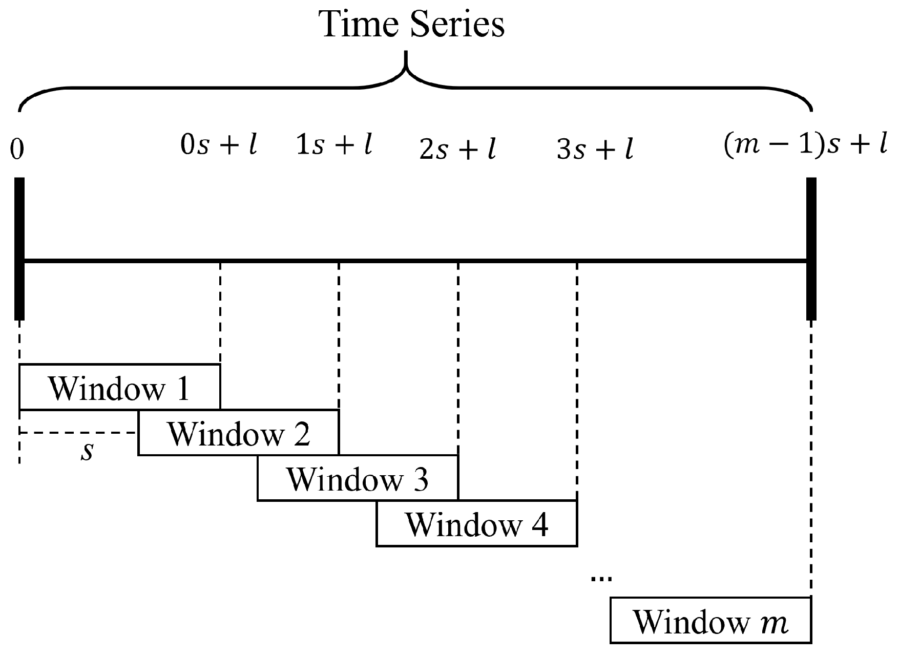
The lattice algorithm is also known as the sliding window method. The concept of the algorithm was proposed by Rubinger in 1974 for the first time [19]. Since it has the advantages of being simplified, easy, operable, practical, and accurate to implement, it has been successfully applied in many fields, such as speech recognition [20], data processing [21], and anomaly detection [22]. Figure 3 shows a simplified diagram of the lattice algorithm. s and l are the step and window sizes, respectively. The window pane of length l slides s to the next window.

3.3. DL Architectures

With the advent of big data, deep learning technology has become an important research hotspot as a perfect performing solution and has been widely applied in image processing [23], natural language processing [24], speech recognition, large language modeling, online advertising, and so on [25]. DL architectures can be divided into supervised learning and unsupervised learning [26]. In supervised learning, the training data are composed of labeled examples, whereas unsupervised learning relies on unlabeled data. In this study, the available data are labeled.
Deep learning was proposed by [25] in 2015. The training process of deep neural networks can be dissected into a series of core steps, each contributing indispensably to the network’s overall efficacy. The first step in building a successful neural network is to collect, clean, and label the data. The second step is network construction. In this study, we chose the MLP [27], RNNs, CNN, and transformer [28] as fundamental DL architectures to experiment with. The GRU model [29] and LSTM [30] are two popular types of RNN architectures that have been widely used in various applications. Subsequently, the training data were input into the network, and the output was calculated using forward propagation. Afterward, the loss function was calculated to measure the difference between the predicted output and the true output. Then, the gradient of each weight and bias was calculated using the backpropagation algorithm based on the value of the loss function. In the next step, an optimization algorithm was used to update the weights and biases of the network based on the gradient direction. Then, the model was validated and adjusted. Lastly, the trained network was tested using the testing set to assess its performance and accuracy.

4. DeepLOCA-Lattice Construction

4.1. Data Description and Preprocessing

The reactor type selected for this research was the PWR, which is the most popular in the world. The dataset used in this study was obtained from our previous work [31] and was generated from the PCTRAN v1.0 software. PCTRAN, a reactor transient and accident simulation software, can be operated on a personal computer. Leveraging a diverse array of mathematical models, PCTRAN facilitates the simulation of nuclear reactor cores and the reactor coolant system during transients and accidents. Its effectiveness has been validated through Fukushima nuclear accident simulations and two operating conditions in our previous work [31], which presents a first-of-its-kind open dataset created using PCTRAN.
PCTRAN is capable of generating an NPP accident dataset based on the type of accident, the severity of the accident, and the simulation time [31]. The generated data are informative, containing 97 parameters such as time stamp, temperature, flow speed, and power. For the LOCA, the dataset comprises various sizes of fault data ranging from 1% to 100% of a 100 cm2 breach in intervals of 1% of 100 cm2. In our previous work, the simulation time was set to longer than 3600 s. The time-step value for the simulation is automatically generated by the PCTRAN software, with a constant interval of 10 s. Following the implementation of equal-interval processing, the sample count for each category experienced a substantial increase from 379, as observed in the original class division, to 8261. In this paper, the structure of the generated data for the LOCA (i.e., 100% of 100 cm2) is depicted in Table 3. Each parameter within the dataset carries distinct physical interpretations. For instance, in Table 3, TAVG corresponds to the temp RCS average, while RRCO signifies the ratio core flow.
In this study, data preprocessing involved two aspects: data standardization and the utilization of the sliding window algorithm to construct the dataset. The PCTRAN simulation provides samples of full-process accident data, while real-world samples are often taken from a specific period. Thus, after employing the PCTRAN simulation data, to align with practical scenarios, we applied the lattice algorithm to partition the dataset along the temporal dimension for data preprocessing, which is more suitable for the requirements of NPPs. The lattice algorithm was used to segment the original data into smaller windows.

4.2. Equal-Interval Partitioning and Data Reconstruction

As described before, the number of breach sizes in the original data is 100. This study provides a method to estimate the fault breach size. However, if the number of categories is 100, a complex, easily over-fitted, time-consuming neural network model will be built [32]. Conversely, a lower number of intervals can more effectively showcase the characteristics and differences of the dataset while mitigating the risk of excessive detail and confusion. Additionally, fewer intervals may enhance the accuracy of subsequent calculations. Thus, this paper proposes dividing the degree of the fault into equally spaced intervals for optimal results.
Given that four is a commonly employed partitioning number [33], it strikes an optimal balance between simplicity and complexity while accurately reflecting data distribution. Therefore, this study divided the PCTRAN simulation data into four intervals with certain representativeness for data description and analysis. Our data were separated into four categories for the subsequent estimation task evenly, where sizes ranging from 1 to 25 cm2, 26 to 50 cm2, 51 to 75 cm2, and 75 to 100 cm2 were each assigned one level.

4.3. Estimation of LOCA Breach Size

To estimate the breach size of the LOCA, DeepLOCA-Lattice designed and constructed a range of popular fundamental deep learning models for testing, including the MLP, RNNs, CNN, and transformer. To assess the adaptability of the simplified neural network model, we deliberately crafted a single-hidden-layer MLP without activation functions. In this article, it is referred to as the simplified MLP.

4.3.1. Multi-Layer Perceptron (MLP)

The MLP, also known as the artificial neural network (ANN), was first proposed by Rosenblatt in 1957 [27]. Subsequently, JL McClell and DE Rumelhart proposed the back propagation (BP) algorithm based on this model, which made the neural network algorithm applicable to nonlinear problems [34]. Ackley et al. introduced the concept of hidden layers and proposed the Boltzmann machine, which led to the idea of a multi-layer perceptron consisting of input, hidden, and output layers [35].
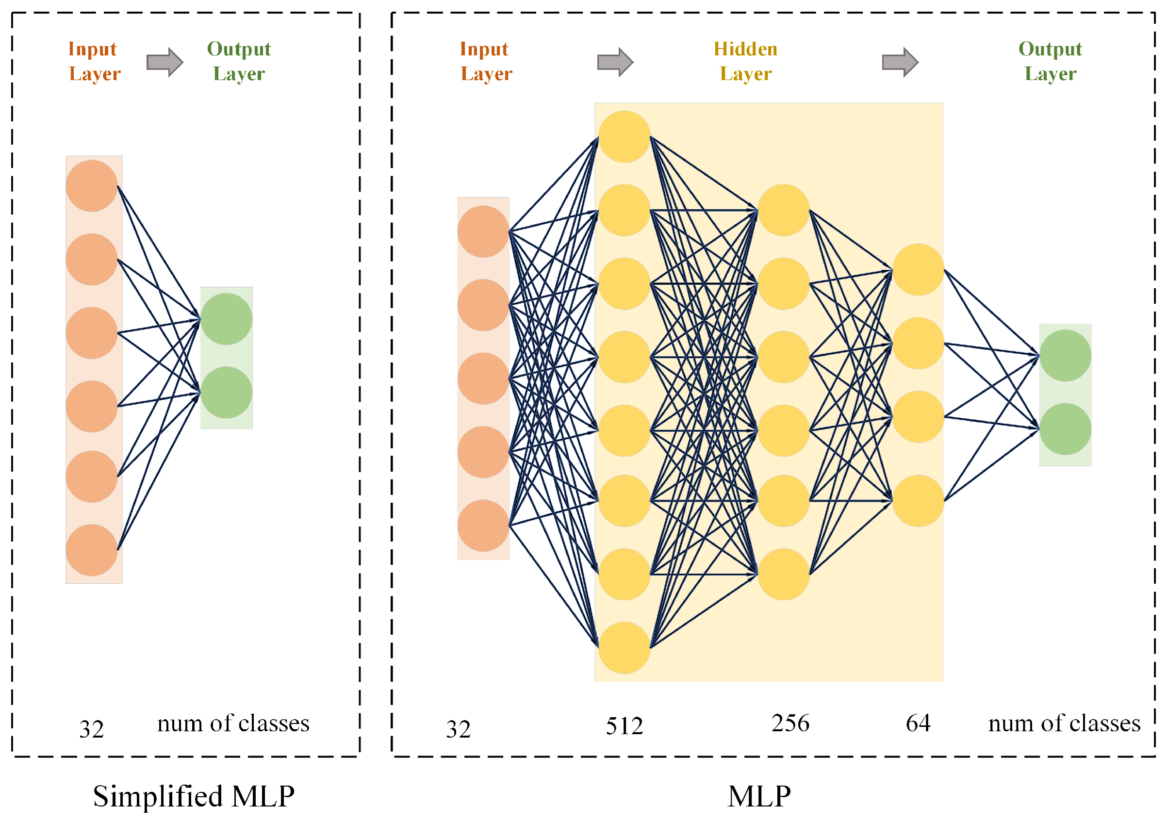
Since the MLP model serves as the fundamental model in deep learning networks, this paper presents the design and construction of both a simplified MLP model and an MLP model. The simplified MLP has emerged as a refined iteration of the traditional MLP architecture, characterized by a solitary hidden layer and a deliberate absence of activation functions. The motivation for developing a simplified model is to explore the adequacy of a straightforward approach in addressing the fault diagnosis of LOCAs. The specific architecture of the simplified MLP model is shown in Figure 4.
The MLP model comprises an input layer, three hidden layers, and an output layer. The input layer has a total of 96 neurons. The number of neurons in each hidden layer is set to 512, 256, and 64, sequentially, while the number of neurons in the output layer remains as 4.

4.3.2. Recurrent Neural Networks (RNNs)

In the processing of temporal data using traditional neural networks, the correlation between temporal data is often ignored. To address this issue, RNNs are proposed and have been widely applied in various fields such as natural language processing (NLP), machine translation, speech recognition, and fault diagnosis [36]. However, because of the problems of gradient explosion and vanishing gradients, RNNs are unable to handle long-term sequences effectively. As a result, researchers introduced improved RNN algorithms, namely, long short-term memory networks (LSTMs) and gated recurrent units (GRUs), which have successfully overcome these issues.
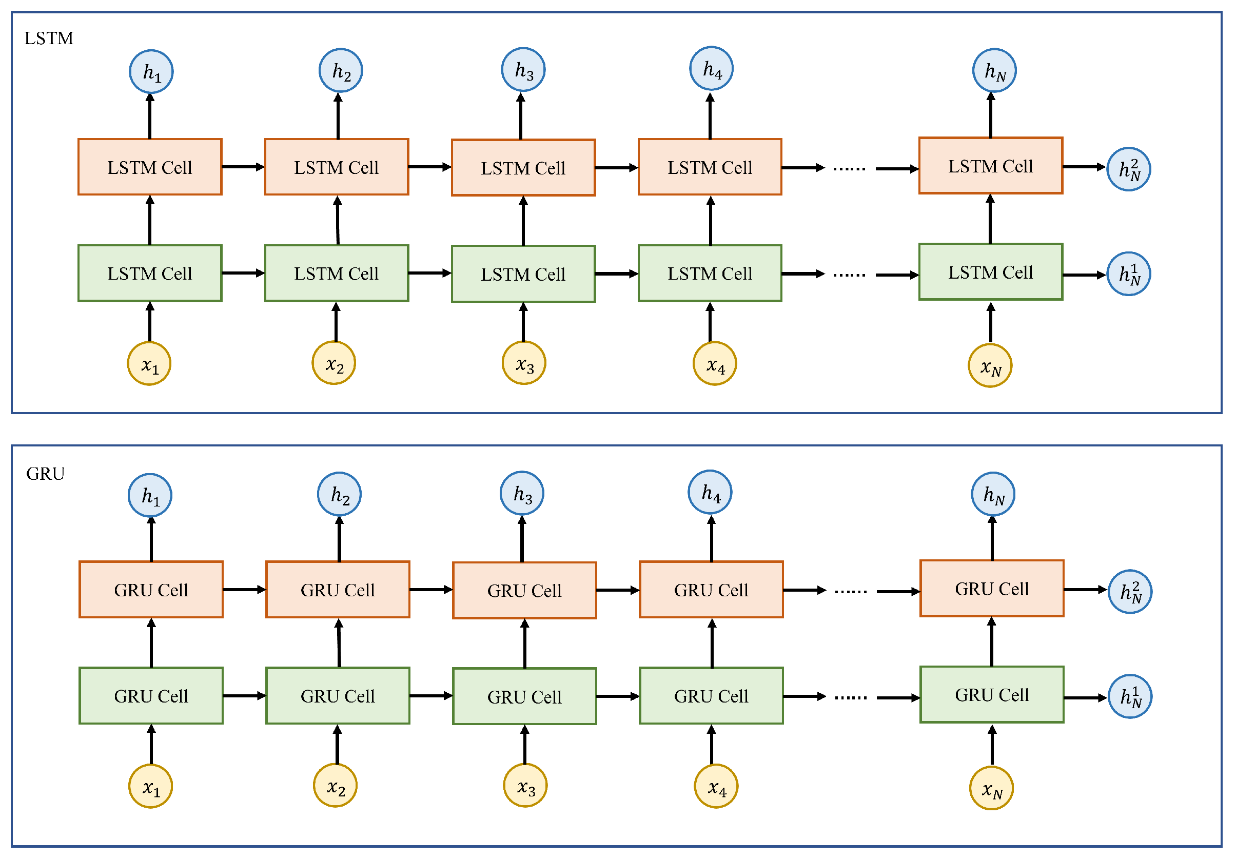
In this study, the dataset consists of time-series data. Therefore, we utilized the RNN model to uncover patterns in predicting and diagnosing the size of the LOCA breach. The aim of this study was to explore the effectiveness of enhanced RNN models, which are LSTM and GRU models, in the task of estimating the LOCA breach size. Figure 5 illustrates the LSTM and GRU network architectures designed in this study. The constructed RNN network architecture includes bidirectional computations, dropout regularization, and batch normalization operations. Specifically, this paper defines two layers of a recurrent neural network with 300 neurons per layer. For example, when using the dataset with four categories and a window pane of 96 adopted in DeepLOCA-Lattice and setting the batch size to 32, the input data shape fed into the RNN network is 32 × 96 × 96 and the output data shape is 32 × 96 × 300. The shape of the hidden state data for the final time step of each layer of the network is 32 × 300. In this study, the hidden state of the final time step of the second layer, i.e., h N 2 , was selected as input for the next stage to predict the classification task. Finally, h N 2 is passed through a batch normalization operation and a linear classifier to output the predicted classification results.

4.3.3. Convolutional Neural Networks (CNNs)

Convolutional neural networks (CNNs), often referred to as ConvNets or convolutional networks, represent a class of deep learning models specially designed for tasks involving grid-structured data, such as images [37], video frames [38], and spatially organized data. As shown in Figure 6, our CNN architecture incorporates convolutional and fully connected layers with appropriate activation functions for feature extraction and classification. It consists of two convolutional layers with ReLU activation. After the convolutional layers, there are two fully connected layers, with ReLU activation in the first and linear transformation in the second. The final layer produces the network output logit without an activation function.

4.3.4. Transformer Model

The transformer model [28], consisting of an encoder and decoder, offers the key advantage of parallel computation. Our DeepLOCA-Lattice-based implementation incorporates a positional encoding layer, two transformer encoder layers, and a linear decoder, as shown in Figure 7. The positional encoding function generates position embedding vectors using the sin–cos formula, and the network weights are initialized before applying transformations to the input data. This process converts the input tensor size from 32 × 96 × 96 to 96 × 32 × 96 while normalizing it. The positional encoding vector is then added to the input data, resulting in a new input vector. The input is then encoded using the transformer encoder based on the set-masked input tensor mask that conceals information from certain positions in the input tensor. Finally, the output of the encoder is decoded linearly to obtain the prediction results.

5. Results and Discussion

The subsequent sections will present scenario predictions and sensitivity analysis of data construction in DeepLOCA-Lattice. Furthermore, we also compared the precision of the models proposed by Choi et al. [9] and Saghafi et al. [14] with the fundamental and simple model in our framework. Choi et al. designed a cascaded fuzzy neural network (CFNN) model, which is a computational framework designed for modeling complex systems using fuzzy logic. It is a T-S FIS model with a specific structure and utilizes genetic algorithm optimization to train and fine-tune the model’s parameters. Saghafi et al. defined a type of recurrent neural network model known as a nonlinear auto-regressive model with exogenous input (NARX). The NARX has an input layer; three hidden fully connected (FC) layers with dimensions of 10, 20, and 10 neurons; and an output layer. Our experiments revealed a particularly intriguing phenomenon. And it is worth noting that our study design incorporates a robust validation strategy, consisting of distinct training, validation, and testing datasets, to ensure an unbiased evaluation of model performance.

5.1. Scenario Deduction

LOCAs are a significant safety concern in NPPs. The size of the breach determines the severity of the accident, and our research provides immediate information on the breach size to help operators minimize consequential damage caused by the LOCA. These findings are expected to contribute significantly to improving the safety standards of NPPs.
In this study, we have employed both grid search and random search techniques for hyperparameter tuning to ensure optimal performance of our deep learning models, as detailed in the strategies implemented. Table 4 presents the hyperparameters of the simplified MLP, MLP, LSTM, GRU, CNN, and transformer models used in DeepLOCA-Lattice. To ensure model convergence, it is crucial to set an appropriate learning rate. A high learning rate can result in gradient explosion, while a low learning rate can lead to overfitting and trap the model in a ‘local optimum’. After conducting multiple experiments, we set the initial learning rate to 0.0001 in this study. The preliminary experiment indicated that the model converges in around 100 iterations. Therefore, we observed convergence progress for 250 iterations. A batch size of 32 was used to optimize the hardware computing resources. Additionally, the dropout rate for the simplified MLP, MLP, and CNN was set to 0. Our optimization process for the LSTM, the GRU model, and transformer models revealed their susceptibility to overfitting. To mitigate this issue and enhance the performance of the model, we introduced a random dropout rate of 0.1 for the three models.
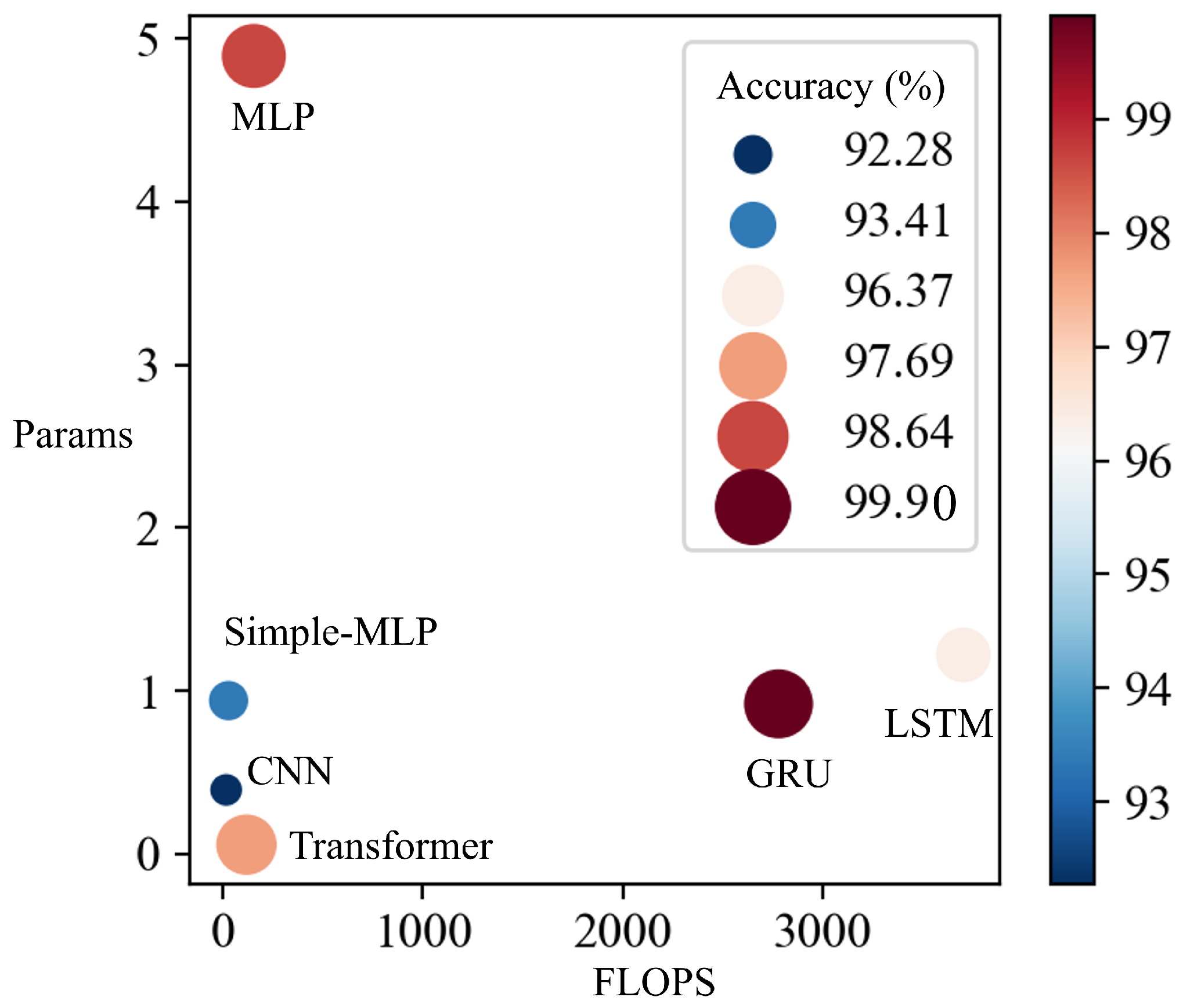
This study analyzed a lattice algorithm with a window size of 96 and a sliding stride of 1. Figure 8 presents a comparative visualization of different neural network architectures in terms of their computational complexity and performance. The x-axis represents the floating-point operations per second (FLOPs), a measure of computational complexity, indicating the number of floating-point operations executed per second by the model. The y-axis displays the logarithmically scaled number of parameters (params) in each model, which is a common proxy for model size or capacity. Each dot represents a distinct neural network architecture, including simplified MLP, MLP, LSTM, GRU, CNN, and transformer. And the size of each dot correlates with the accuracy percentage of the respective model, as denoted by the color bar on the right side of the graph.
Models positioned towards the bottom left corner, such as the transformer, indicate lower computational complexity and a smaller number of parameters, while those towards the top right indicate higher computational complexity and a higher number of parameters. The color gradient from blue to red illustrates a scale from lower to higher accuracy, suggesting that models with more FLOPs and params tend to achieve higher accuracy, with the GRU model marked by the largest and darkest dot reflecting the highest accuracy among the compared models. Our results show that all models achieved high accuracy rates, exceeding 90%. Among these models, the GRU model achieved the highest accuracy rate of 99.90%, followed by the transformer model with an accuracy of 99.69%. The MLP, LSTM, simplified MLP, and CNN achieved accuracies of 98.64%, 96.87%, 93.41%, and 92.28%, respectively.
To visualize the neural network’s classification process, a random sample from the 76–100 cm2 LOCA break size area is selected. Figure 9 illustrates this using a multi-layer MLP, presented as a probabilistic heat map across the four layers. The axes represent the transformation of a one-dimensional vector into a two-dimensional space, indicating positional data rather than physical dimensions. The color intensity correlates with higher probability values.
The data processing in the MLP starts with the first fully connected layer (fc1), enhancing the dimensionality to 512. Subsequently, it traverses the second layer (fc2), reducing the dimensionality to 256, and then the third layer (fc3), further decreasing to 128 dimensions. Considering our four-class classification task, the final fourth layer (fc4) output is a four-dimensional vector. The map shows the highest probability value at position (1,1), accurately classifying the break size in the 76–100 cm2 range, aligning with actual conditions.
Additionally, we have replicated the NARX of Saghafi et al. and the CFNN of Choi et al. Saghafi et al. that primarily revolve around nonlinear programming, a domain that deviates from our research emphasis on neural networks, and the result of the NARX was 36.46%. We also found that the execution time of the NARX was considerably prolonged. The NARX would require approximately 7 h on a GeForce RTX 3080 Ti GPU, whereas our model typically completes within a range of 1 to 3 h. Otherwise, the optimal accuracy of Choi’s CFNN is merely 35.48%, which is less than half of the accuracy rate achieved by the simplified MLP in our proposed DeepLOCA-Lattice. Therefore, we draw an intriguing and substantial inference. That is, the complexity of the model structure does not invariably correlate with an improvement in its accuracy, which means that even a simple single model can effectively perform the fault diagnosis significantly.
As shown in Table 5, in terms of the FLOPs-to-params (FLOPs/params) ratio, the simplified MLP, MLP, and NARX exhibit proximity, both hovering around 32, indicating a balance achieved between computational efficiency and model capacity. On the contrary, LSTM and the GRU model demonstrate significantly higher FLOPs-to-params ratios compared to the other models, signifying their elevated computational complexity and potentially necessitating greater computational resources. On the other hand, the CNN exhibits a relatively high FLOPs-to-params ratio, indicating its outstanding computational efficiency. Similarly, the transformer boasts a comparably high FLOPs-to-params ratio, suggesting an equilibrium attained between computational efficiency and model capacity. As for CFNN, it is incapable of calculating FLOPs. The estimation of FLOPs (floating-point operations) necessitates an enumeration of the floating-point arithmetic operations per computational act. Within a CFNN, the operations are restricted to matrix manipulations and fuzzy logic computations. Fuzzy logic operations diverge from the standard linear algebraic operations and do not subscribe to a fixed FLOP count. These findings suggest that networks of the same type display consistency between their number of parameters and floating-point numbers relative to each other. These observations provide insight into the resource requirements and performance aspects of various deep learning models used in LOCA breach size diagnosis.
The superior performance of the GRU and transformer models can be attributed to their stronger modeling and memory capabilities, allowing them to handle more complex data relationships and sequences. Surprisingly, the relatively simplified MLP and MLP models also performed well in this fault diagnosis task, suggesting the presence of smaller nonlinear relationships among different LOCA breach sizes. As for RNNs, LSTM is more prone to gradient vanishing and exploding problems due to the introduction of three gate units (input gate, output gate, and forget gate) to filter and process the input data, making training difficult and increasing the likelihood of encountering gradient issues. In contrast, the GRU model only uses two gate units (update gate and reset gate), reducing computational complexity, improving training efficiency, and minimizing the risk of gradient vanishing and exploding. Moreover, the GRU model is better suited for processing small batches of data compared to LSTM. These findings have significant implications for selecting appropriate deep learning models for breach size diagnosis in LOCAs.
Notably, the accuracy of the model is ascertained not from the training or test sets but rather from a separate validation set. This method ensures a more unbiased evaluation of the model’s performance on unseen data, thus providing a more realistic gauge of its generalization capabilities. Furthermore, in subsequent sections, we delve deeper by conducting sensitivity analysis, altering various sample parameters within the data. Such an analysis is instrumental in understanding how different factors influence the model’s performance and in identifying potential areas of improvement or vulnerabilities in the modeling process.

5.2. Sensitivity Analysis

In this study, we conducted an in-depth discussion and analysis of the impact of key data construction parameters on model performance. These parameters included various window sizes, sliding stride sizes, and equal-interval partitions. The goal is to identify critical parameters in the dataset that significantly affect model performance. Our findings provide insight into the optimal configurations of the dataset for the DL models used in the diagnosis of LOCA breach size and have important implications for enhancing safety standards in NPPs.

5.2.1. Window Size and Sliding Stride

This paper presents a comprehensive analysis that compares different window sizes and sliding strides using the simplified MLP, MLP, LSTM, GRU, CNN, and transformer models. The objective is to identify the optimal window parameters for computing performance. Specifically, we evaluated window sizes of 10 and 96 with stride values of 1 and 5, as well as data without lattice operations. Table 6 provides detailed parameter selections for each dataset.
Our analysis reveals that when using a window size of 96 and a stride of 1, all models demonstrate optimal performance in terms of accuracy. This is because this configuration enables a more comprehensive and complete representation of sequence data by leveraging temporal information to a greater extent. As a result, this configuration improves both the accuracy and generalizability of the models, making it ideal for LOCA breach size diagnosis tasks in NPPs.
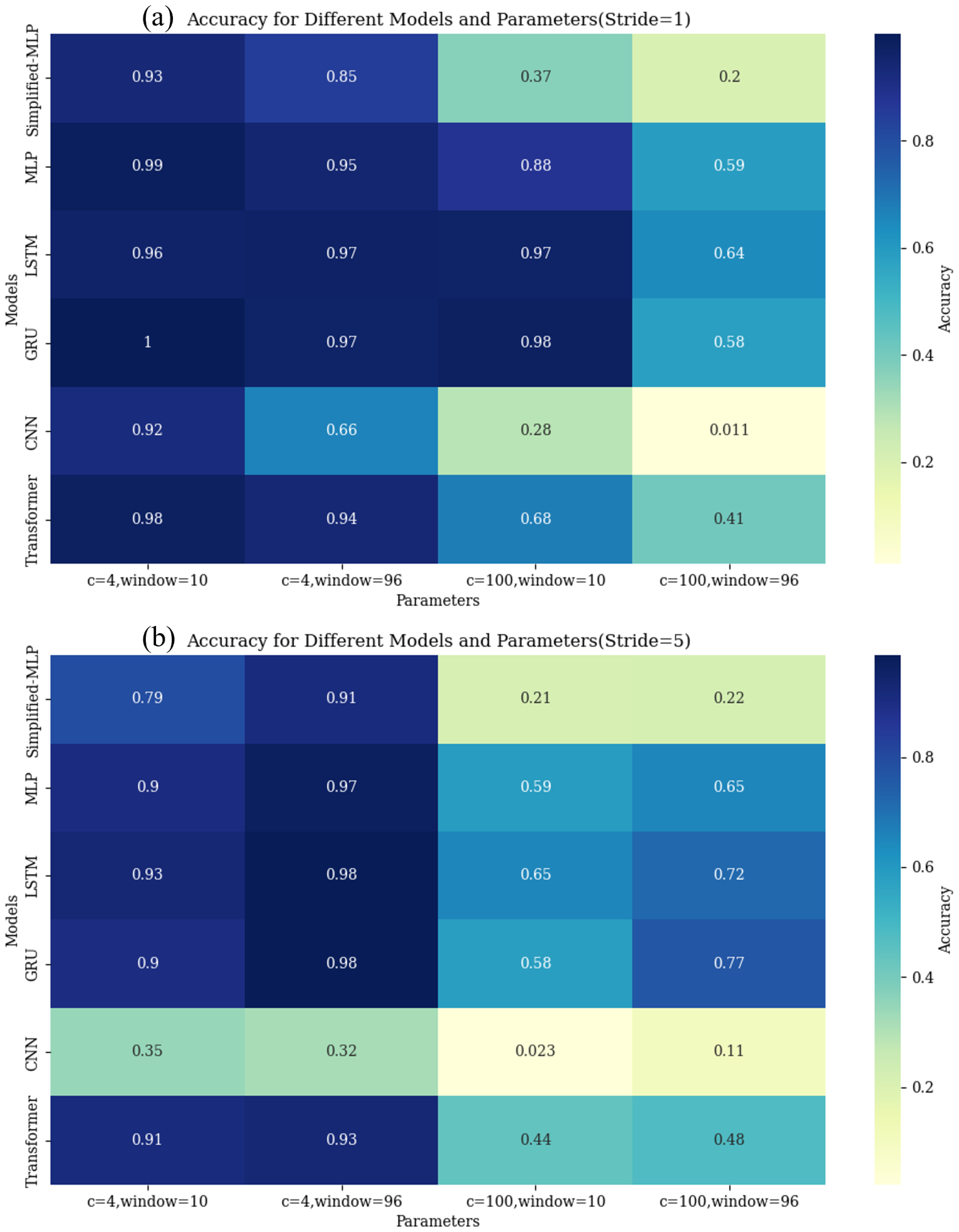
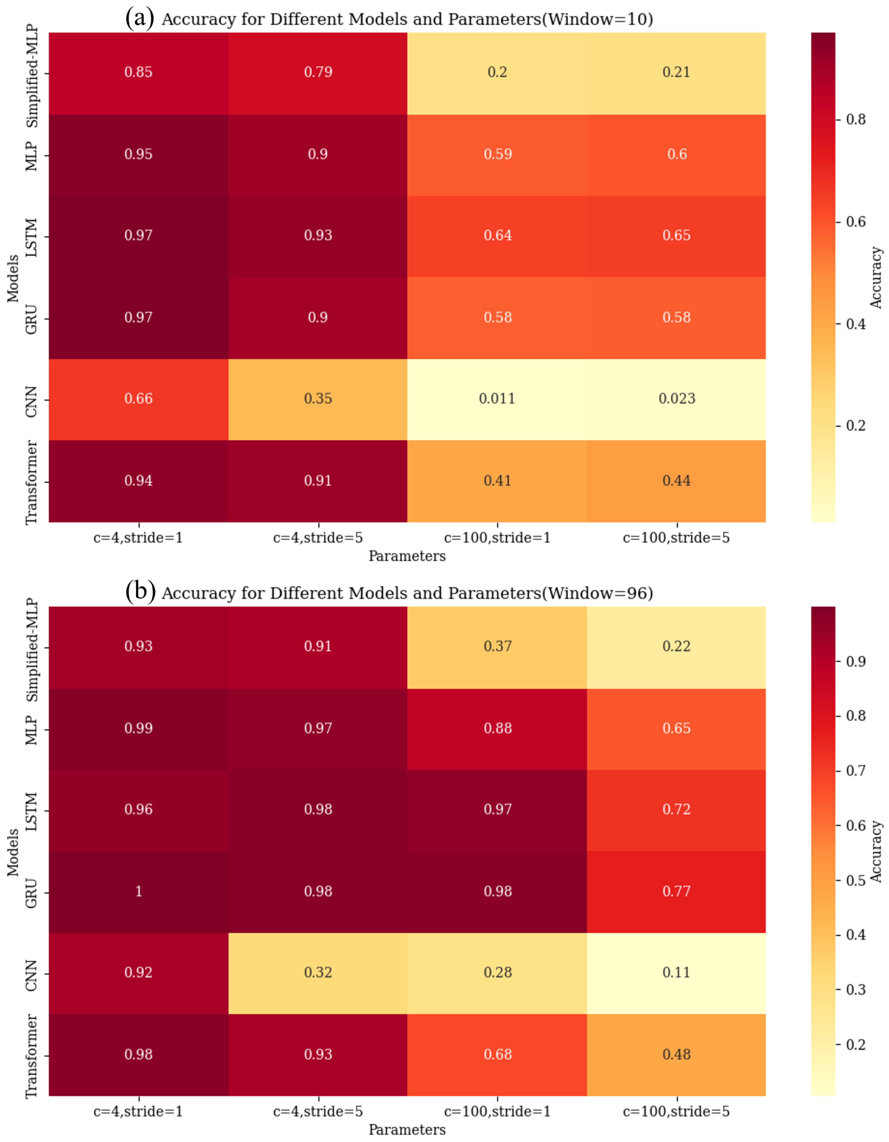
Figure 10 and Figure 11 provide a comprehensive analysis of the model accuracy across different sliding stride and window sizes. In these figures, ‘c’ denotes the number of categories, ‘c = 4’ represents the model accuracy after reconstructing category divisions, and ‘c = 100’ corresponds to the model accuracy without any category division.
As illustrated in Figure 10, in addition to the CNN, when the sliding stride is held constant, there exists a positive correlation between the model accuracy and window size. Irrespective of whether the number of categories is 4 or 100, increasing the window size improves the accuracy of all models under the stride = 5 and stride = 1 conditions. Although increasing the window size results in a reduction in the number of samples, it concurrently amplifies the continuity of information within each sample. Consequently, for the diagnosis of LOCA breach size in NPPs, stronger continuity in individual sample sequences and higher information entropy significantly contribute to the model’s enhanced reasoning capabilities. However, for the CNN model, in the case where the stride is 5 and the number of categories is 4, the model accuracy decreases as the window size increases. This also indicates that larger window sizes do not necessarily lead to higher model accuracy, and this is also dependent on the model characteristics and the number of categories.
When considering a fixed window size, as depicted in Figure 11, the model accuracy demonstrates a negative correlation with the sliding stride for a data category of 4. Decreasing the sliding stride size leads to an increase in the number of samples, thus contributing to improved model reasoning. However, for a data category of 100, with a sliding window size of 10, reducing the sliding stride size from 5 to 1 results in a slight decrease in model accuracy. Conversely, when the sliding window size is set to 96, decreasing the stride from 5 to 1 significantly enhances the model’s accuracy. These findings imply that in scenarios where sample information is limited, simply increasing the number of samples may not be as effective as enriching the information content within individual samples.
It is well known that model precision demonstrates a positive correlation with window size and a negative correlation with sliding stride size [39]. However, in the context of diagnosing the size of the LOCA breach in NPPs, there exists a nuanced relationship among the number of window sizes, the number of categories, and the sliding stride through our experiments. The relationship between them is not simply a straightforward positive or negative correlation.

5.2.2. Diagnostic Scales

In this study, we investigated the impact of size-equivalent partitioning on the entire model framework by applying both graded and non-graded partitioning methods to scale the data. The data are divided into two scales, which are the graded 4-category scale and the non-graded 100-category scale.
Table 7 presents the average improvement factors for the simplified MLP, MLP, LSTM, GRU, CNN, and transformer models on different diagnostic scales. The analysis reveals that the diagnosis accuracy of the graded scale is higher than the non-graded. This indicates that there is an enhancement in model accuracy after size-equivalent partitioning. The results demonstrate that the CNN model shows the highest improvement factor, reaching 19.92, followed by the simplified MLP, which achieves 3.63. The third position is held by the transformer model, with an improvement factor of 1.94. Lastly, the MLP, LSTM, and GRU models are quite similar, all hovering around 1.4 in terms of the improvement factor.
The significant improvement in the accuracy of the CNN is attributable to the advantageous structure of the convolutional and pooling layers, facilitating feature extraction. The structure of the simplified MLP may lead to lower computation, especially when dealing with data with simpler structures, hence achieving a higher improvement factor. The transformer and MLP models follow closely. Their complexity and larger number of parameters may impose limitations on their improvement factor. Finally, the LSTM and the GRU model exhibit similar improvement factors. Their memory capabilities enable them to effectively capture long-term dependencies in time-series data. As a result, the potential for accuracy improvement is smaller for the LSTM and GRU models.
In the contemporary landscape of statistical analysis within the realm of computational sciences, the Friedman test has emerged as a robust non-parametric alternative to the one-way ANOVA with repeated measures. It is particularly adept at discerning significant discrepancies across multiple treatment conditions when the dependent variable being measured is ordinal. The test is predicated on the ranks of data rather than their raw values, thus it is intrinsically immune to the parametric assumptions of normality and homogeneity of variances that often constrain the applicability of parametric tests.
The Friedman test is most efficacious when employed to evaluate the performance across a suite of computational models or algorithms that have been subjected to a series of experimental conditions. As shown in Table 8, upon the application of the Friedman test, comprising the performance results of multiple models, the derived test statistic stands at 33.5663. This statistic, which follows a chi-squared distribution under the null hypothesis, is a measure of the overall divergence among the model ranks. Accompanying this statistic, the p-value obtained is 3.1048 × 10 6 . This is significantly below the conventional alpha threshold of 0.05, unequivocally indicating that we can reject the null hypothesis with a high degree of confidence.
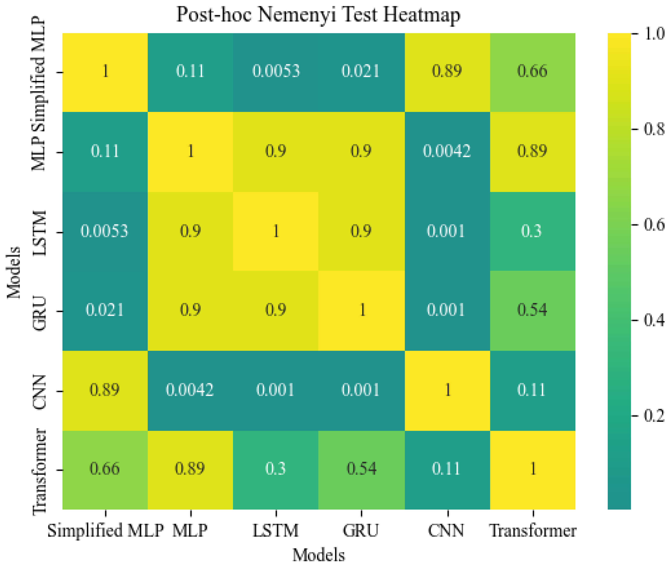
In conclusion, the results of the Friedman test are indicative of statistically significant differences in the performance of the evaluated models. Furthermore, we use the post hoc Nemenyi test to assess the differences between groups. As shown in Figure 12, there is a matrix of p-values indicating the statistical significance of differences between pairs of models. The colors range from dark to light, with darker shades representing lower p-values, and thus, more significant differences between model performances. The color bar on the right-hand side indicates the scale of significance levels. It can be interpreted from the heatmap that the comparison between the GRU and CNN models results in a very low p-value (0.001), shown by the dark color, suggesting a statistically significant difference in their performance rankings. Conversely, the comparison between the LSTM and GRU models, with a p-value of 0.9, is represented by a much lighter color, indicating no significant difference between these two models’ rankings.

6. Conclusions

In NPPs, the early and accurate diagnosis of LOCA breach size is crucial for effective emergency response. This study proposes an effective LOCA breach size diagnosis framework (DeepLOCA-Lattice) to experiment with different data construction approaches and fundamental deep learning models. The main conclusions are as follows:
  • The complexity of a model does not necessarily equate to its performance. In this study, even the simplest deep learning models can achieve accuracy rates that exceed 90% in LOCA breach size diagnoses, while the accuracy of the complex CFNN and NARX models is less than 40%. On the other hand, the high accuracy of 90% also underscores the idealized nature of the PCTRAN simulated data, emphasizing the necessity of considering the disparity between simulated and real data in genuine research endeavors.
  • The findings reveal the existence of an intricate relationship among diagnostic scales, sliding window size, and sliding stride. It is not the case that larger sliding windows and smaller stride lengths consistently yield higher model accuracy. Specific outcomes are also influenced by factors such as the number of categories and the precise architecture of the model. For instance, as discussed in Section 5.2.1, in the scenario where the number of categories is four and the stride is 5, increasing the window size results in a decrease in the model accuracy. In contrast, with a window size of 10 and 100 categories, reducing the stride leads to an increase in the accuracy of the model.
  • Our analysis reveals that when using a window size of 96 and a stride of 1, all models demonstrated optimal performance in terms of accuracy. This can serve as a reference for the construction of datasets for subsequent LOCA breach size estimation models. Researchers can attempt to use smaller window sizes with larger stride sizes for LOCA breach size diagnosis.
Our proposed DeepLOCA-Lattice framework exhibits versatile applicability across multiple domains. Specifically, it thrives in environments characterized by high dimensionality, such as applications producing voluminous data akin to the sensors in NPPs. Its robust design excels in scenarios necessitating critical fault detection, where timely and precise diagnoses are paramount to averting catastrophic outcomes or substantial economic repercussions. Additionally, the technology within our architecture renders it adept at handling temporal data sequences, making it particularly apt for time-series data or sequential datasets. Furthermore, the framework is designed for conducting in-depth ablation studies, catering to domains where dissecting the influence of individual components or parameters is imperative for further optimization and refinement.
These results have significant implications for the improvement of safety standards in NPPs and contribute to the development of more advanced and reliable fault diagnosis methods in nuclear energy systems. While the DeepLOCA-Lattice framework exhibits commendable performance with simulated datasets, its applicability to real-world scenarios from nuclear power plants (NPPs) remains a subject of inquiry. The inherent variability and noise prevalent in data sourced from NPPs could substantially influence the model’s accuracy and reliability, signaling a limitation in the study due to the absence of extensive real-world validation and testing. Given that our data are derived from simulation models, future researchers might consider introducing noise or leveraging data trend variations in order to align the diagnostic process more closely with real-world scenarios.

Author Contributions

Writing—original draft preparation and formal analysis, X.X.; investigation, methodology, and visualization, X.X. and P.C.; data curation and conceptualization, B.Q.; software, X.X., B.Q. and P.C.; validation, X.X., B.Q., J.L., Q.D. and J.T.; writing—review and editing, project administration, supervision, and resources, J.L., Q.D. and J.T.; funding acquisition, J.L. All authors have read and agreed to the published version of the manuscript.

Funding

The research was supported by the Innovation Funds of CNNC–Tsinghua Joint Center for Nuclear Energy R&D (Project No. 20202009032) and a grant from the National Natural Science Foundation of China (Grant No. T2192933).

Data Availability Statement

The data that support the findings of this study are available upon request from the corresponding author.

Conflicts of Interest

The authors declare no conflict of interest.

References

  1. Qi, B.; Zhang, L.; Liang, J.; Tong, J. Combinatorial techniques for fault diagnosis in nuclear power plants based on Bayesian neural network and simplified Bayesian network-artificial neural network. Front. Energy Res. 2022, 10, 920194. [Google Scholar] [CrossRef]
  2. Lee, S.; Kim, J.; Arigi, A.M.; Kim, J. Identification of Contributing Factors to Organizational Resilience in the Emergency Response Organization for Nuclear Power Plants. Energies 2022, 15, 7732. [Google Scholar] [CrossRef]
  3. Lin, Y.; Zhang, W.J. Towards a novel interface design framework: Function–behavior–state paradigm. Int. J. Hum.–Comput. Stud. 2004, 61, 259–297. [Google Scholar] [CrossRef]
  4. Lin, Y.; Zhang, W.J. A function-behavior-state approach to designing human–machine interface for nuclear power plant operators. IEEE Trans. Nucl. Sci. 2005, 52, 430–439. [Google Scholar] [CrossRef]
  5. Yamanouchi, A. Effect of core spray cooling in transient state after loss of coolant accident. J. Nucl. Sci. Technol. 1968, 5, 547–558. [Google Scholar] [CrossRef]
  6. Zhang, C.; Chen, P.; Jiang, F.; Xie, J.; Yu, T. Fault Diagnosis of Nuclear Power Plant Based on Sparrow Search Algorithm Optimized CNN-LSTM Neural Network. Energies 2023, 16, 2934. [Google Scholar] [CrossRef]
  7. Qi, B.; Liang, J.; Tong, J. Fault Diagnosis Techniques for Nuclear Power Plants: A Review from the Artificial Intelligence Perspective. Energies 2023, 16, 1850. [Google Scholar] [CrossRef]
  8. She, J.; Shi, T.; Xue, S.; Zhu, Y.; Lu, S.; Sun, P.; Cao, H. Diagnosis and prediction for loss of coolant accidents in nuclear power plants using deep learning methods. Front. Energy Res. 2021, 9, 665262. [Google Scholar] [CrossRef]
  9. Choi, G.P.; Yoo, K.H.; Back, J.H.; Na, M.G. Estimation of LOCA breach Size Using Cascaded Fuzzy Neural Networks. Nucl. Eng. Technol. 2017, 49, 495–503. [Google Scholar] [CrossRef]
  10. Wang, Y.; Liu, R.; Lin, D.; Chen, D.; Li, P.; Hu, Q.; Chen, C.L.P. Coarse-to-fine: Progressive knowledge transfer-based multitask convolutional neural network for intelligent large-scale fault diagnosis. IEEE Trans. Neural Netw. Learn. Syst. 2021, 34, 761–774. [Google Scholar] [CrossRef]
  11. Mandal, S.; Santhi, B.; Sridhar, S.; Vinolia, K.; Swaminathan, P. Nuclear power plant thermocouple sensor-fault detection and classification using deep learning and generalized likelihood ratio test. IEEE Trans. Nucl. Sci. 2017, 64, 1526–1534. [Google Scholar] [CrossRef]
  12. Yao, Y.; Wang, J.; Long, P.; Xie, M.; Wang, J. Small-batch-size convolutional neural network based fault diagnosis system for nuclear energy production safety with big-data environment. Int. J. Energy Res. 2020, 44, 5841–5855. [Google Scholar] [CrossRef]
  13. Wang, H.; Peng, M.; Ayodeji, A.; Xia, H.; Wang, X.; Li, Z. Advanced fault diagnosis method for nuclear power plant based on convolutional gated recurrent network and enhanced particle swarm optimization. Ann. Nucl. Energy 2021, 151, 107934. [Google Scholar] [CrossRef]
  14. Saghafi, M.; Ghofrani, M. Real-time estimation of break sizes during LOCA in nuclear power plants using NARX neural network. Nucl. Eng. Technol. 2019, 51, 702–708. [Google Scholar] [CrossRef]
  15. Xu, Y.; Lin, K.; Hu, C.; Wang, S.; Wu, Q.; Zhang, L.; Ran, G. Deep transfer learning based on transformer for flood forecasting in data-sparse basins. J. Hydrol. 2023, 625, 129956. [Google Scholar] [CrossRef]
  16. El-Shafeiy, E.; Alsabaan, M.; Ibrahem, M.; Elwahsh, H. Real-Time Anomaly Detection for Water Quality Sensor Monitoring Based on Multivariate Deep Learning Technique. Sensors 2023, 23, 8613. [Google Scholar] [CrossRef]
  17. Liapis, C.M.; Kotsiantis, S. Temporal Convolutional Networks and BERT-Based Multi-Label Emotion Analysis for Financial Forecasting. Information 2023, 14, 596. [Google Scholar] [CrossRef]
  18. Islam, M.M.; Islam, M.Z.; Asraf, A.; Al-Rakhami, M.S.; Ding, W.P.; Sodhro, A.H. Diagnosis of COVID-19 from X-rays using combined CNN-RNN architecture with transfer learning. Benchcouncil Trans. Benchmarks Stand. Eval. 2022, 2, 100088. [Google Scholar] [CrossRef]
  19. Zaki, M.J.; Hsiao, C.J. Efficient algorithms for mining closed itemsets and their lattice structure. IEEE Trans. Knowl. Data Eng. 2005, 17, 462–478. [Google Scholar] [CrossRef]
  20. Yang, Z.; Yang, H.; Chang, C.-C.; Huang, Y.; Chang, C.-C. Real-time steganalysis for streaming media based on multi-channel convolutional sliding windows. Knowl.-Based Syst. 2022, 237, 107561. [Google Scholar] [CrossRef]
  21. Yaroslavsky, L.P.; Egiazarian, K.O.; Astola, J.T. Transform domain image restoration methods: Review, comparison, and interpretation. Nonlinear Image Process. Pattern Anal. XII 2001, 4304, 155–169. [Google Scholar]
  22. Chang, C.-I.; Wang, Y.; Chen, S.-Y. Anomaly detection using causal sliding windows. IEEE J. Sel. Top. Appl. Earth Obs. Remote Sens. 2015, 8, 3260–3270. [Google Scholar] [CrossRef]
  23. Rubinger, B. Performance of a sliding window detector in a high interference air traffic environment. In Proceedings of the IEEE Conference on Computer Vision and Pattern Recognition, Las Vegas, NV, USA, 27–30 June 2016. [Google Scholar]
  24. Kłosowski, P. Deep learning for natural language processing and language modelling. In Proceedings of the 2018 Signal Processing: Algorithms, Architectures, Arrangements, and Applications (SPA), Poznań, Poland, 19–21 September 2018. [Google Scholar]
  25. LeCun, Y.; Bengio, Y.; Hinton, G. Deep learning. Nature 2015, 521, 436–444. [Google Scholar] [CrossRef] [PubMed]
  26. Baker, B.; Gupta, O.; Naik, N.; Raskar, R. Designing neural network architectures using reinforcement learning. arXiv 2016, arXiv:1611.02167. [Google Scholar]
  27. Rosenblatt, F. The perceptron: A probabilistic model for information storage and organization in the brain. Psychol. Rev. 1958, 65, 386. [Google Scholar] [CrossRef]
  28. Vaswani, A.; Shazeer, N.; Parmar, N.; Uszkoreit, J.; Jones, L.; Gomez, A.N.; Kaiser, Ł.; Polosukhin, I. Attention is all you need. Adv. Neural Inf. Process. Syst. 2017, 30, 1–11. [Google Scholar]
  29. Chung, J.; Gulcehre, C.; Cho, K.; Bengio, Y. Empirical evaluation of gated recurrent neural networks on sequence modeling. arXiv 2014, arXiv:1412.3555. [Google Scholar]
  30. Hochreiter, S.; Schmidhuber, J. Long short-term memory. Neural Comput. 1997, 9, 1735–1780. [Google Scholar] [CrossRef]
  31. Qi, B.; Xiao, X.; Liang, J.; Po, L.; Zhang, L.; Tong, J. An open time-series simulated dataset covering various accidents for nuclear power plants. Sci. Data 2022, 9, 766. [Google Scholar] [CrossRef]
  32. Schmidhuber, J. Deep learning in neural networks: An overview. Neural Netw. 2015, 61, 85–117. [Google Scholar] [CrossRef]
  33. Ostrand, T.J.; Balcer, M.J. The category-partition method for specifying and generating fuctional tests. Commun. ACM 1988, 31, 676–686. [Google Scholar] [CrossRef]
  34. McClell, J.L.; Rumelhart, D.E.; PDP Research Group. Parallel Distributed Processing, Volume 2: Explorations in the Microstructure of Cognition: Psychological and Biological Models; MIT Press: Cambridge, MA, USA, 1987. [Google Scholar]
  35. Ackley, D.H.; Hinton, G.E.; Sejnowski, T.J. A learning algorithm for Boltzmann machines. Cogn. Sci. 1985, 9, 147–169. [Google Scholar]
  36. Bao, Y.; Wang, B.; Guo, P.; Wang, J. Chemical process fault diagnosis based on a combined deep learning method. Can. J. Chem. Eng. 2022, 100, 54–66. [Google Scholar] [CrossRef]
  37. Arena, P.; Basile, A.; Bucolo, M.; Fortuna, L. Image processing for medical diagnosis using CNN. Nucl. Instruments Methods Phys. Res. Sect. Accel. Spectrometers Detect. Assoc. Equip. 2003, 497, 174–178. [Google Scholar] [CrossRef]
  38. Saponara, S.; Elhanashi, A.; Gagliardi, A. Real-time video fire/smoke detection based on CNN in antifire surveillance systems. J. Real-Time Image Process. 2021, 18, 889–900. [Google Scholar] [CrossRef]
  39. Beane, S.R.; Bedaque, P.F.; Parreno, A.; Savage, M.J. Two nucleons on a lattice. Phys. Lett. B 2004, 585, 106–114. [Google Scholar] [CrossRef]
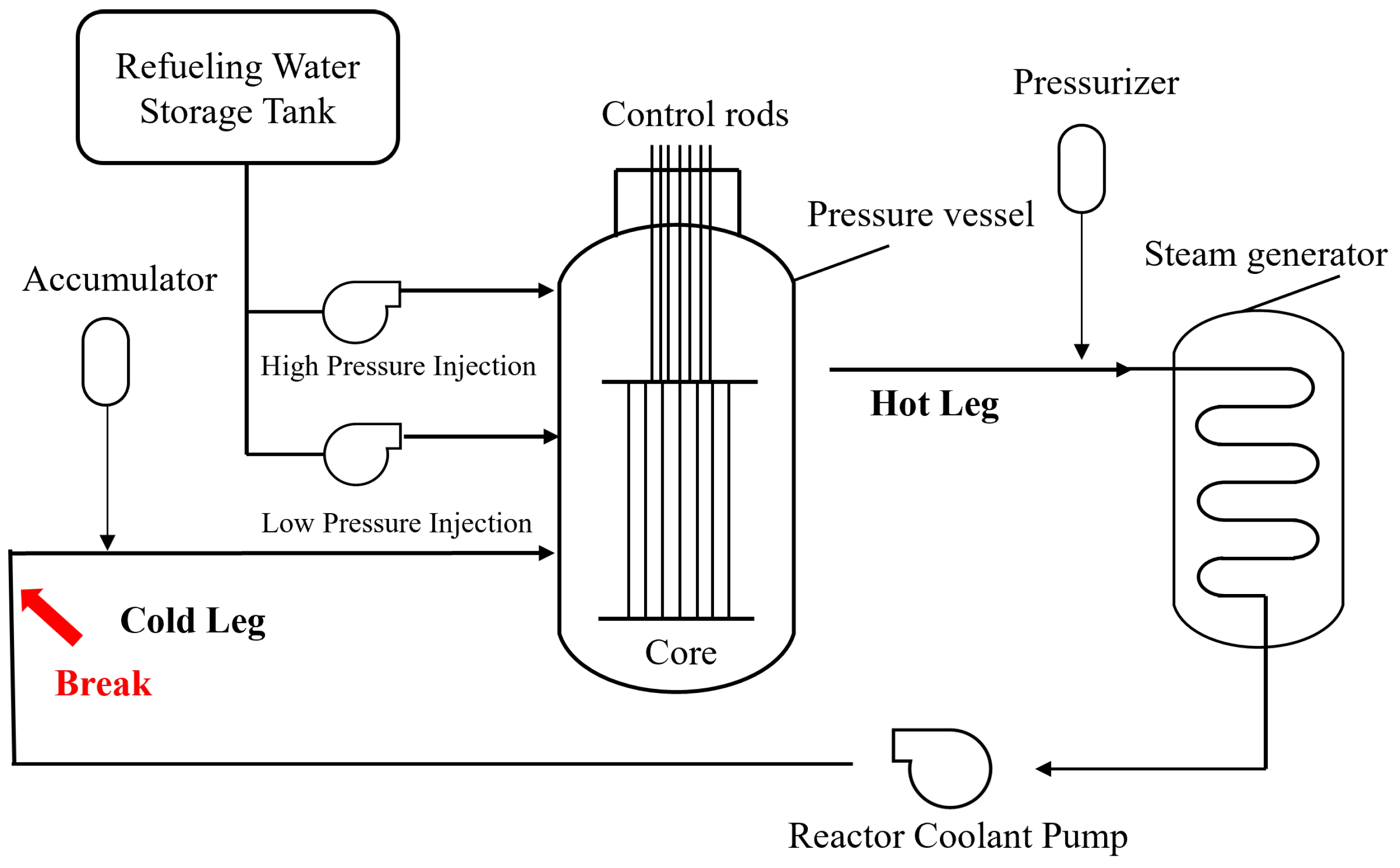
Figure 1. A schematic representation of a LOCA in a nuclear reactor.
Energies 17 00159 g001
Figure 2. Structure of proposed DeepLOCA-Lattice framework. The proposed DeepLOCA-Lattice framework consists of four main stages: stage I: data collection and preprocessing, stage II: expanding the diagnostic scale, stage III: model building, and stage IV: estimation of the LOCA breach size.
Energies 17 00159 g002
Figure 3. A diagram of the lattice algorithm.
Energies 17 00159 g003
Figure 4. Simplified MLP and MLP diagrams of DeepLOCA-Lattice framework.
Energies 17 00159 g004
Figure 5. LSTM and GRU of DeepLOCA-Lattice framework.
Energies 17 00159 g005
Figure 6. CNN of DeepLOCA-Lattice framework.
Energies 17 00159 g006
Figure 7. Transformer of DeepLOCA-Lattice framework.
Energies 17 00159 g007
Figure 8. Results of DeepLOCA-Lattice framework.
Energies 17 00159 g008
Figure 9. Heat map of LOCA break size (78 cm2) during four-layer MLP processing. In the fc4 results, the coordinate (0,0) represents a LOCA break size area of 1–25 cm2, (1,0) indicates 26–50 cm2, (0,1) signifies 51–75 cm2, and (1,1) denotes 76–100 cm2.
Energies 17 00159 g009
Figure 10. The accuracy of different models for data of various categories and window sizes: (a) The distribution of model accuracy for different categories and different window sizes when the sliding stride is fixed at 1. (b) The distribution of model accuracy for different categories and different window sizes when the sliding stride is fixed at 5.
Energies 17 00159 g010
Figure 11. The accuracy of different models for data of various categories and sliding strides: (a) The distribution of model accuracy for different categories and different window strides when the window size is fixed at 10. (b) The distribution of model accuracy for different categories and different sliding strides when the window size is fixed at 96.
Energies 17 00159 g011
Figure 12. Friedman test results highlighting significant differences in model performance.
Energies 17 00159 g012
Table 1. Notation and abbreviations.
IndexParameter NameParameter Abbreviation
1Loss-of-coolant accidentLOCA
2Simplified multi-layer perceptronSimplified MLP
3Multi-layer perceptronMLP
4Long short-term memoryLSTM
5Gated recurrent unitGRU
6Convolutional neural networkCNN
7Deep learningDL
8Nuclear power plantsNPPs
9Deep learning framework for LOCA breach size diagnosis based on the lattice algorithmDeepLOCA-Lattice
10Pressurized water reactorPWR
Table 2. Overview of existing work.
AuthorMain Work
She et al. [8]Integrated CNN, LSTM, and ConvLSTM for diagnosing and predicting LOCAs. Demonstrated functionality, accuracy, and divisibility.
Choi et al. [9]Employed a cascaded fuzzy neural network (CFNN) for estimating LOCA breach sizes.
Wang et al. [10]Proposed a PKT algorithm for extracting more generalized fault information in NPP fault diagnosis and intelligent construction of a coarse-to-fine knowledge structure.
Mandal et al. [11]Utilized a deep belief network (DBN) for classifying fault data in NPPs.
Yao et al. [12]Optimized CNNs with small-batch-size processing for assembly in NPP diagnostic systems.
Wang et al. [13]Developed a highly accurate and adaptable fault diagnosis technique using CGRU and improved particle swarm optimization (EPSO).
Saghafi et al. [14]Defined a nonlinear auto-regressive model with exogenous input (NARX) for diagnosing LOCA breach sizes.
Table 3. The time series of the status parameters with a 1% of 100 cm2 break of LOCA.
TimePTAVGTHARRCOWFLB
0155.5000310.0000327.82401.00000
10155.4682309.9801327.80551.00000
20155.4674309.9777327.81051.00000
30155.4719309.9802327.81121.00000
40155.4711309.9779327.81141.00000
4710157.0756292.0552292.29951.06210
4720157.0776292.0528292.29701.06210
4730157.1084292.0511292.29441.06210
4740157.0882292.0486292.29191.06210
Table 4. Neural network hyperparameter optimization.
HyperparameterNumber
Learning rate0.0001
Number of iterations250
Batch size32
Table 5. Model metrics comparison.
ModelFLOPsParams (MB)FLOPs/ParamsAccuracy (%)
Simplified MLP30.67080.940132.6593.41
MLP157.20454.893532.1198.64
LSTM3702.4021.22023031.2396.37
GRU2778.95880.92023019.4599.90
CNN18.91530.392948.1892.28
Transformer120.32410.05682119.2997.69
NARX0.04610.001531.0536.46
CFNN/0.0066/35.48
Table 6. Various window sizes and stride values.
IndexWindowStride
1101
2105
3961
4965
5none
Table 7. The accuracy distribution of different models across varying numbers of categories.
ModelNumber of CategoriesStride = 5
Window = 10
Stride = 5
Window = 96
Stride = 1
Window = 96
Stride = 1
Window = 10
Average Factor
Simplified MLP479.08%91.23%93.41%84.59%3.63
10021.33%22.09%36.90%20.38%
MLP490.46%96.63%98.64%95.17%1.46
10059.70%64.92%87.67%58.64%
LSTM492.81%98.48%96.37%96.95%1.33
10064.83%72.01%96.70%64.34%
GRU489.90%98.48%99.90%96.63%1.38
10058.21%76.56%97.86%57.98%
CNN434.55%31.98%92.28%66.04%19.92
1002.31%10.56%28.22%1.13%
Transformer490.97%92.55%97.69%93.79%1.94
10043.66%47.55%67.66%40.59%
Table 8. The results of the Friedman test.
Friedman Test Statisticp-Value
33.5663 3.1048 × 10 6
Disclaimer/Publisher’s Note: The statements, opinions and data contained in all publications are solely those of the individual author(s) and contributor(s) and not of MDPI and/or the editor(s). MDPI and/or the editor(s) disclaim responsibility for any injury to people or property resulting from any ideas, methods, instructions or products referred to in the content.